Article

Self-Supervised Condition Monitoring for Wind Turbine Gearboxes Based on Adaptive Feature Selection and Contrastive Residual Graph Neural Network

1
College of Artificial Intelligence, Harbin Institute of Technology, Shenzhen, Shenzhen 518055, China
2
Institute of Green and Low-Carbon Energy Innovation, Harbin Institute of Technology, Shenzhen, Shenzhen 518055, China
*
Author to whom correspondence should be addressed.
Energies 2025, 18(20), 5474; https://doi.org/10.3390/en18205474
Submission received: 27 August 2025 / Revised: 26 September 2025 / Accepted: 30 September 2025 / Published: 17 October 2025

Abstract

Frequent failures in wind turbines underscore the critical need for accurate and efficient online monitoring and early warning systems to detect abnormal conditions. Given the complexity of monitoring numerous components individually, subsystem-level monitoring emerges as a practical and effective alternative. Among all subsystems, the gearbox is particularly critical due to its high failure rate and prolonged downtime. However, achieving both efficiency and accuracy in gearbox condition monitoring remains a significant challenge. To tackle this issue, we present a novel adaptive condition monitoring method specifically for wind turbine gearbox. The approach begins with adaptive feature selection based on correlation analysis, through which a quantitative indicator is defined. With the utilization the selected features, graph-based data representations are constructed, and a self-supervised contrastive residual graph neural network is developed for effective data mining. For online monitoring, a health index is derived using distance metrics in a multidimensional feature space, and statistical process control is employed to determine failure thresholds. This framework enables real-time condition tracking and early warning of potential faults. Validation using SCADA data and maintenance records from two wind farms demonstrates that the proposed method can issue early warnings of abnormalities 30 to 40 h in advance, with anomaly detection accuracy and F1 score both exceeding 90%. This highlights its effectiveness, practicality, and strong potential for real-world deployment in wind turbine monitoring applications.

1. Introduction

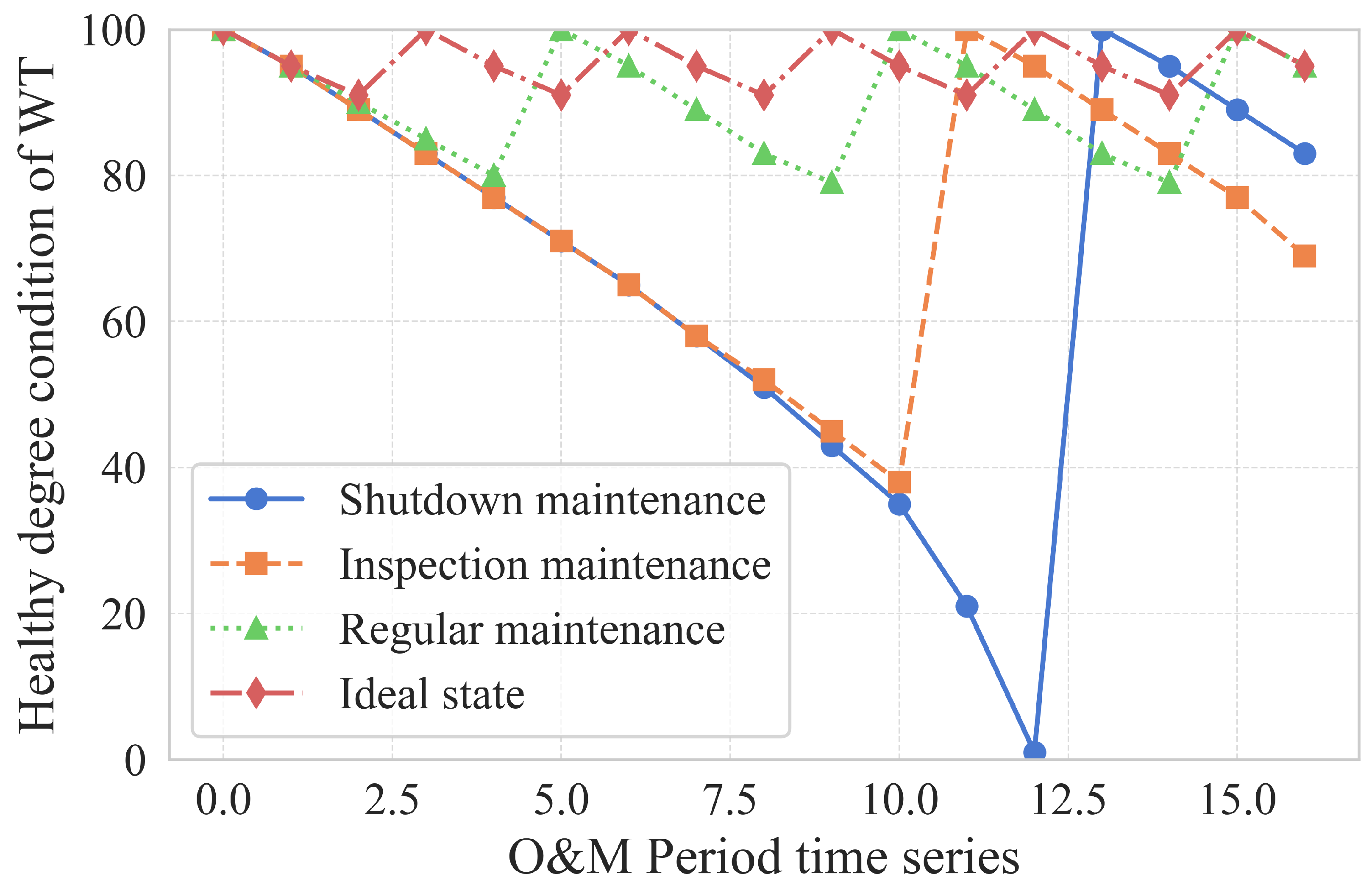
Due to the harsh environments in which wind turbines (WTs) operate, failures occur frequently, resulting in a heightened demand for operation and maintenance (O&M). Traditional O&M strategies, including shutdown, inspection, and regular maintenance, affect the health condition of WTs in varying ways [1], as illustrated in Figure 1.
Each inflection point represents a manual maintenance intervention. In essence, the revenue generated via a wind farm is proportional to the area under the curves. Ideally, it is crucial to maintain wind turbines (WTs) in a consistently high condition of health. Among various O&M strategies, shutdown has the most detrimental impact on wind farm efficiency. Although inspection is less disruptive, it is constrained by high labor and material costs, as well as low operational efficiency. Regular maintenance also faces cost-efficiency challenges and often results in ineffective investment due to unnecessary servicing of normally functioning WTs. Gradually, predictive maintenance has emerged as a promising alternative, offering a cost-effective and efficient approach by enabling accurate detection of abnormal WTs and timely forecasting of potential failures.
A critical task in predictive maintenance is the accurate identification of inflection points, which necessitates a precise definition of the condition of WTs. Therefore, it is essential to develop an efficient, automated, and intelligent O&M method, along with a condition monitoring (CM) method [2], which supports the early identification of critical information before the occurrence of anomalies or failures. This approach minimizes unnecessary losses and provides maintenance personnel with sufficient time for proactive intervention.
CM is fundamentally based on anomaly detection (AD) [3], which plays a crucial role in industrial processes by enhancing quality control and improving product qualification rates [4]. In the wind power industry, AD is primarily employed in O&M to identify sudden or unexpected anomalies [5]. Using both supervised [6] and unsupervised [7] methods, AD detects anomalies in individual wind turbine components instantaneously. The key distinction between CM and AD lies in scope and temporal focus: while AD identifies short-term abnormal patterns, CM continuously evaluates the condition of components over a longer time horizon, providing a more comprehensive understanding of equipment health.
The application of traditional model-based and signal-processing-based CM is often constrained due to the complexity of modeling difficulty and high implementation costs. In contrast, data-driven CM provides an effective approach to extracting valuable insights from WT data. Capturing the coupling effects among multiple variables enables the identification of patterns corresponding to different operational conditions. Leveraging pattern recognition techniques, data-driven CM supports end-to-end monitoring. More importantly, it can detect and extract micro-level features before anomalies become perceptible to maintenance personnel, allowing for early fault warnings [8,9,10]. Additionally, when implemented using supervisory control and data acquisition (SCADA) systems, it eliminates the need for additional sensors or hardware, thereby enhancing internal system reliability while reducing O&M costs [11,12]. Consequently, data-driven CM has become a widely accepted and practical solution in the wind power industry.
With its various features, SCADA provides a relatively intuitive description of the operational processes for WT [13,14]. However, significant dynamic fault characteristics may be lost as the time intervals between data points are relatively long, typically around 10 min. This limitation can be addressed using intelligent methods that possess powerful learning and data mining capabilities.
Extensive research has been conducted to monitor WT conditions, primarily focusing on either the entire WT system or specific individual components. Detecting anomalies in the entire system often leads to inefficiencies and high labor costs. Moreover, data collected from operational wind farms are typically unlabeled, making it challenging to obtain component-specific operational data. Extracting data for individual components from numerous features is a difficult and highly labor-intensive process that requires extensive research. Additionally, the lifespan of WTs is predominantly influenced by key components, while other components have a lesser impact. Therefore, it is essential to develop adaptive CM and anomaly analysis methods that specifically target the critical subsystems of WTs. Statistically, among the various subsystems, the gearbox is the most critical when considering both failure rates and downtime caused by failures [15].
Traditional condition monitoring methods that rely on vibration analysis based on signal processing face the challenge of high computational costs. Additionally, the original signals often contain significant noise, resulting in a low signal-to-noise ratio, which severely limits the effectiveness of vibration analysis in condition monitoring tasks. Furthermore, the conventional simple threshold methods based on SCADA data introduce substantial uncertainty during the modeling process, leading to a high false alarm rate and significantly reduced accuracy, thereby impairing overall condition monitoring performance.
CM for WT gearbox is often hindered by the lack of an effective model and framework, which limits its practical application in the wind industry [16]. To address this, a normal behavior model [17] is proposed, comprising the following key steps: feature selection, model training, difference comparison, and condition monitoring. First, a machine learning model is trained using raw data obtained from healthy operating conditions. Next, unknown data requiring monitoring are input into the pretrained model. The results are then compared with corresponding healthy-condition data. Smaller differences indicate that the monitored data sample closely resembles a healthy condition. A failure threshold is established based on these differences to quantitatively detect anomalies in WTs. However, existing CM methods suffer from low accuracy and efficiency due to random feature selection, low accuracy in abnormal condition recognition, an insufficient consideration of feature correlations during model training, and uncertainty in difference calculation.
Feature selection for condition monitoring can be classified into subjective methods and objective methods [18]. The former relies on personal experience and prior literature to manually identify features related to the target subsystem [19,20]. However, subjective methods can lead to information loss due to inherent biases [21]. For example, the SCADA system can only describe the operational conditions of wind turbines from the perspective of sensor networks, but it lacks the precision to provide a comprehensive overview. Consequently, subjectively selecting variables as model inputs introduces substantial uncertainty. Additionally, some valid variables may be overlooked, resulting in the loss of valuable information during model training. Therefore, objective methods, which quantitatively identify relevant features based on computational relationships [22,23,24], have been more widely adopted by researchers. These methods often use various correlation coefficients, such as the Pearson coefficient [25], maximal information coefficient [26], and Kendall coefficient [27]. This approach effectively eliminates subjective biases and uncertainties, preserves the maximum amount of useful information in the data, ensures proper training of the model, and enables high-accuracy anomaly detection. However, different coefficients vary in their applicable ranges, and their applications are limited to specific scenarios, an aspect that has not been sufficiently addressed.
Machine learning plays a significant role in extracting, recognizing, and modeling various conditions within a multidimensional space [28]. According to the training process, it can be classified into supervised [29], semi-supervised [30], and unsupervised [31] methods. However, considering the lack of labeled data, the insufficiency of effective samples, the discrepancies between data and features, and the uncertainty in describing the conditions of WT in real-world WT condition monitoring, a self-supervised method [32,33], which is similar to unsupervised learning, has attracted increasing attention due to its ability to automatically construct supervisory information from unlabeled data [34,35]. Self-supervised learning uses the data itself as labels to generate self-supervised signals, allowing the model to learn representations by predicting missing parts, perturbations, or correlations in the data [36,37]. Under the self-supervised framework, specific models play a crucial role. Among them, graph neural networks (GNNs) [38] are particularly noteworthy due to their unique architecture. By representing data as nodes and edges, GNN can effectively model and learn the characteristics of raw data, addressing the differences among various features in the raw SCADA system and capturing the correlations among them.
Healthy conditions are modeled using a model trained on historical healthy data. Data from unknown conditions are represented as graphs and processed through the pretrained model. Subsequently, a comparison is made between the corresponding results obtained from healthy-condition data and unknown-condition data. Commonly used metrics for comparison include residuals [39,40], the root mean square error [26], square prediction error [41], Mahalanobis distance [42,43], and Kantorovich distance [44]. Based on the distance metrics, a numerical representation is constructed to describe the healthy condition of the subsystem and provide a threshold for determining failures. The health index (HI) is often established using an exponentially weighted moving average (EWMA) [45], and the failure threshold is determined according to the 3 σ principle or statistical process control (SPC) [46]. When the HI exceeds this threshold, the subsystem is considered abnormal, and a warning is issued.
In summary, within the context of low anomaly recognition, traditional CM performs poorly in both accuracy and efficiency due to the high cost of CM, subjective factors in feature selection, random factors in method application, and the lack of consideration of feature correlations. Specifically, the manual separation for feature selection overlooks the correlations between features. And there is an absence of specific standards that target subsystems in quantitative selection. This results in high labor costs and significant variability, leading to low efficiency and reliability. Additionally, the weak expressive power and low accuracy of models often stem from inefficiencies caused by manually labeled data during deep model training, as well as the tendency of basic models to overlook feature differences and correlations. Moreover, residuals for specific target features can only reflect subsystem conditions from a single perspective during prediction and discrepancy calculation, making them susceptible to subjective biases. The overall reliability is further compromised due to the challenge of representing subsystem conditions with a single-dimensional measurement. To address these limitations, an adaptive condition-monitoring method based on SCADA data for wind turbine gearboxes is proposed. The main contributions are as follows:
  • Modified normal behavior model-based wind turbine gearbox condition monitoring.
  • Correlation-based adaptive feature selection with a quantitative indicator defined.
  • Optimized self-supervised contrastive residual graph neural network for data mining.
  • Generalized healthy index and adaptive failure threshold for condition monitoring.
  • Ninety-percent-plus recognition accuracy and 40 h’ advance warning for 2 real SCADA datasets.
This paper is structured as follows. Section 2 presents the methodology applied at each step, including five subsections: feature selection, model training, health index, failure threshold, and the overall online condition monitoring system. Section 3 presents the experimental process conducted on two datasets for validation, along with relevant applications and discussions. Finally, Section 4 concludes the paper and outlines prospects for future works.

2. Methodology

An adaptive condition-monitoring method, adaptive feature selection and self-supervised contrastive residual graph neural network (AFS-CRGN), is proposed in this paper for a wind turbine gearbox. For data preparation, AFS is initially developed by analyzing correlations between features, with a quantitative indicator established. To facilitate data mining and model training, a self-supervised CRGN model is designed. After this, online monitoring begins for the gearbox HI, which is established using distance metrics in multidimensional space and EWMA. Based on the HI, a failure threshold is established using SPC. Finally, online condition monitoring of the wind turbine gearbox is realized.

2.1. Adaptive Feature Selection Based on Correlation Analysis

AFS aims to identify suitable data features for the CM task through correlation analysis. This analysis determines the degree of relationship between features by examining the correlation coefficients among various data features.
The Anderson–Darling test is performed to assess whether each feature of the raw SCADA data follows a normal distribution. However, none of the variables follow a normal distribution, rendering the Pearson correlation coefficient unsuitable. Therefore, the Spearman coefficient is employed, as shown in Equation (1), where d i represents the difference in ranks for each pair of observations, and n represents the total number of observations.
ρ = 1 6 i = 1 n d i 2 n ( n 2 1 )
Manually and directly selected features typically exhibit high randomness and are prone to introducing subjective factors. This creates significant uncertainty for the condition monitoring task of wind turbine gearboxes. To prevent the introduction of excessive subjective factors and mitigate the impact of random factors on the results, the adaptive feature selection is proposed. Some core features are selected firstly based on the industry experience as they are the most relevant to the target sub-system, gearbox. Then, the correlations between the remaining features and such core features are evaluated to select the most appropriate features for condition monitoring. In detail, five features closely associated with the gearbox are identified as core features based on previous research, the primary functions of the gearbox, and O&M reports from wind farms (only for Case I), as shown in Table 1. The rotor speed and generator speed represent the rotational speeds of the low-speed shaft and high-speed shaft of the gearbox, respectively.
For each core feature, the Spearman correlation coefficients between the remaining features and the core features are calculated. Each remaining feature is correlated with five core features, and the average of the results obtained is taken as the degree of similarity of that feature. For each feature excluding the core, the following equation applies.
ρ = 1 5 i = 1 5 ρ i
where ρ represents the correlation coefficients of remaining features with respect to the core features. Subsequently, a quantitative indicator is established. The variable indices with correlation coefficients exceeding this indicator correspond to those strongly correlated variables. These variables, combined with the core features, constitute the raw data samples used for model training. The quantitative indicator is a key parameter, and the number of adaptively selected variables varies, depending on its value. Typically, it ranges from 0.5 to 0.8. In this paper, it is set to 0.6 based on the experiments and discussions presented in Section 3. After feature selection, the selected data undergoes min–max normalization to eliminate dimensionality effects, as shown in Equation (3).
x i = x i x min x max x min
Through the above AFS, the data for subsequent model training is prepared. Adaptive refers to the fact that the feature selection method proposed in this article provides a framework that can autonomously select features for different wind turbines and operating conditions.This ensures the generalization of the method, allowing for feature selection on a larger scale. Compared to the traditional recursive feature elimination method and the importance-based feature selection method, the proposed AFS can operate independently, without the need to bind subsequent tasks to this part of the content or the need for complex computations. Based on the actual physical meaning of core features determination, it starts from the data itself and uses the relationships among data for calculations. The proposed AFS can lower the subjective factors in feature selection, making it more efficienct in wind turbine gearbox condition monitoring. It is efficient and simple, and it can adaptively adjust dynamically, making it suitable for promotion and use in real industrial scenarios.

2.2. Model Training Based on Contrastive Residual Graph Neural Network

Once the data is prepared, model training is conducted to learn specific representations from the data and its samples. In this section, the data sampling and model training methods are presented.
As a type of deep learning model, GNN takes into account the correlations between different features of raw data. This study focuses on the CM task of WT gearbox. The selected features through AFS exhibit significant correlations. Using raw data directly for model training overlooks these inter-feature correlations, resulting in suboptimal training performance. Self-supervised learning uses the data itself as labels to generate self-supervised signals, allowing the model to learn representations by predicting missing parts, perturbed information, or correlations in the data. The gearbox monitoring data used in this study comes from the SCADA system of the wind farm and consists of a high-dimensional, non-stationary time series. Without effective labeled samples, self-supervised learning methods can extract useful information from a large amount of unlabeled data and complete model training. In addition, contrastive learning can further enhance the robustness of the model by employing data augmentation strategies to maintain invariance to noise and operational fluctuations in sensor system data. Therefore, a CRGN based on GNN and self-supervised contrastive learning is constructed as the foundational model for data mining and model training.
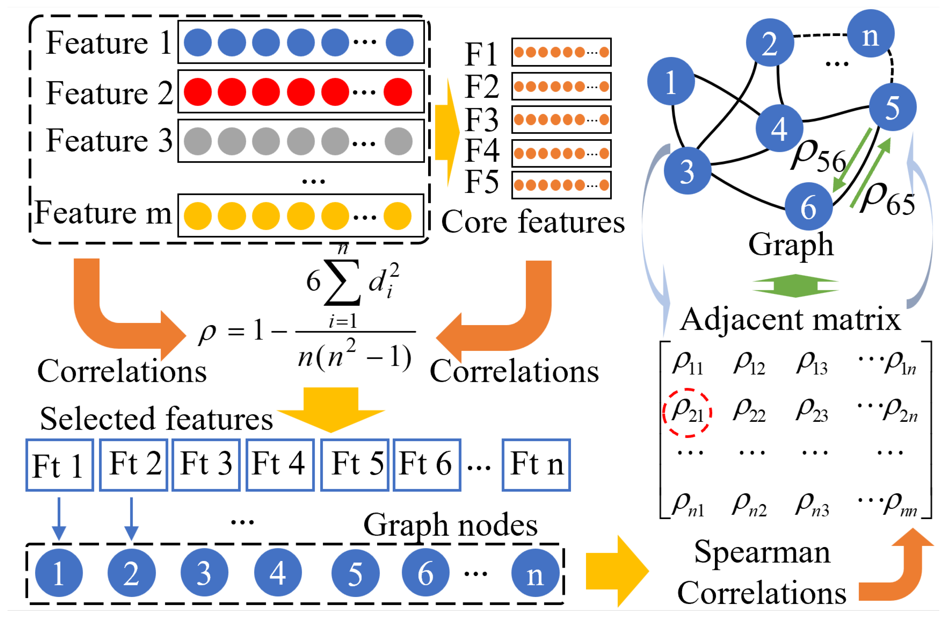
The data samples used for CRGN are referred to as graph samples, which include raw data and the correlation relationships among different features. Each feature is represented as a node, while the correlations among features are represented as edges. Based on the Spearman coefficients between features, an adjacency matrix is constructed, as shown in Equation (4), where ρ represents the Spearman coefficients between different features.
A = ρ 11 ρ 12 ρ 13 ρ 1 n ρ 21 ρ 22 ρ 23 ρ 2 n ρ n 1 ρ n 2 ρ n 3 ρ n n
The formation of the graph data samples is illustrated in Figure 2, where F1 to F5 represent the core features, and Ft 1 to Ft n denote the selected features based on AFS.
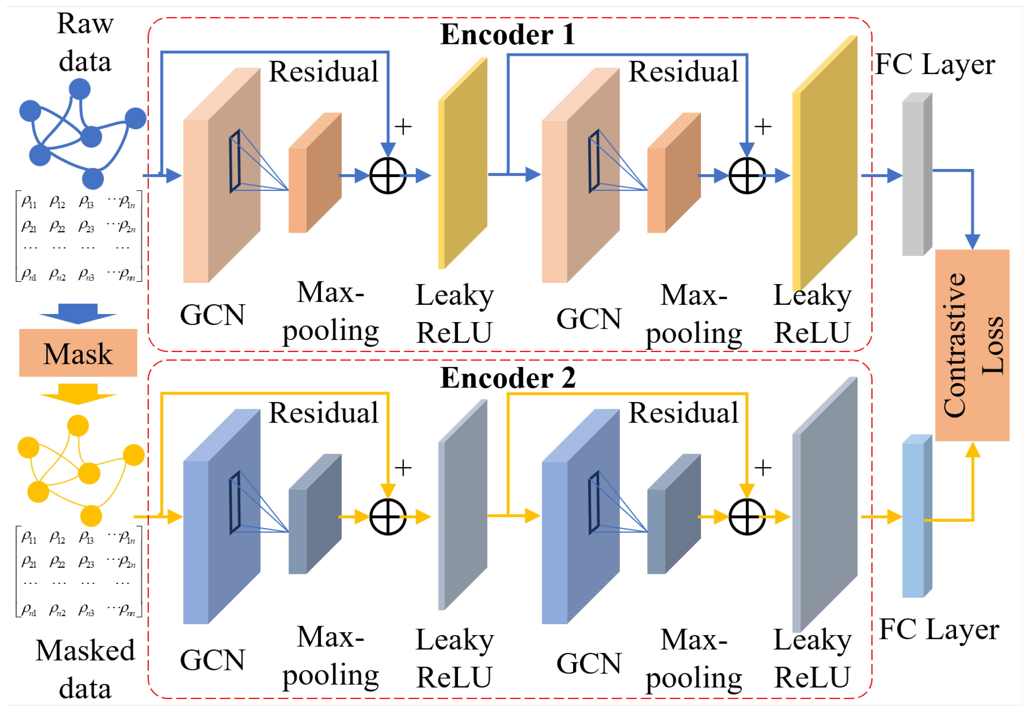
The CRGN constructed in this study consists of four graph convolutional layers, each referred to as a graph convolutional network (GCN) layer. By combining the advantages of GNNs and convolutional neural networks, it is well-suited for performing the CM task and generating graph samples. A GCN is a class of neural network designed to operate on graph-structured data. It extends the concept of convolution from grid-like data, such as images, to graphs by aggregating features from neighboring nodes, thereby capturing both local and global structural information. A common formulation for a GCN layer is given by Equation (5).
H ( l + 1 ) = σ ( D ˜ 1 2 A ˜ D ˜ 1 2 H ( l ) W ( l ) )
where H ( l ) represents the feature matrix at the l - t h layer, with H ( 0 ) = X as the input features. A ˜ represents the adjacency matrix with added self-connections, as shown in Equation (6). D ˜ represents the diagonal degree matrix of A ˜ , defined as shown in Equation (7). W ( l ) represents the trainable weight matrix at layer l. σ ( · ) represents activation function.
A ˜ = A + I
D ˜ i i = j A ˜ i j
The Leaky-ReLU is used as the activation function, with the negative slope coefficient set to 0.1. Additionally, residual connections are implemented to preserve information integrity. Under a self-supervised learning framework, two encoders are constructed for contrastive learning. The raw data is masked by Gaussian random noise, with a standard deviation of 0.1. Both the raw and masked data are input into the two encoders. The contrastive loss-based objective function is presented as Equation (8).
L = 1 N i = 1 N log exp ( sim ( z i , z i + ) / τ ) exp ( sim ( z i , z i + ) ) / τ + j = 1 K exp ( sim ( z i , z i j ) / τ ) + λ | | w | | 2 2
where z i represents the feature representation. z i + and z i j represent the positive and negative samples, respectively. sim ( x , y ) refers to the cosine similarity. τ signifies the temperature parameter that determines the shape. The stochastic gradient descent (SGD) optimizer with Nesterov momentum is treated as optimization, along with L2-regularization. Model framework is shown in Figure 3.
After model training, the health feature representations are learned from data samples. The trained models are then deployed to the online monitoring system to participate in condition monitoring.

2.3. Healthy Index Based on Distance Metric

Under the same data preprocessing and sampling methods, graph samples for the target gearbox under monitoring are constructed. After loading the CRGN model trained with healthy data, the unknown condition samples are input into the pre-trained model. Based on distance metrics, a similarity comparison is performed on the obtained results. Then, HI is established to characterize the varying health conditions of the WT gearbox.
Since relying on a single distance metric introduces randomness, multiple distance metrics are employed to mitigate the impact of this variability on the results, such as the Manhattan distance d M , Euclidean distance d E , cosine similarity d c o s , and Chebyshev distance d C h . The average of these distances, d a v g , is considered the mean distance between healthy samples and samples with unknown conditions. The formulas used to calculate each metric are expressed as Equations (9)–(13) below, where x and y represent the two vectors involved in the distance calculations, and Normed indicates that the results have been normalized.
d M ( x , y ) = i = 1 n | x i y i |
d E ( x , y ) = i = 1 n ( x i y i ) 2
d c o s ( x , y ) = i = 1 n x i y i i = 1 n x i 2 i = 1 n y i 2
d C h ( x , y ) = max ( | x i y i | )
d a v g = N o r m e d [ 1 4 ( d M + d E + d c o s + d C h ) ]
According to EWMA and normalized average distance, HI is established for the gearbox. The weighted moving average assigns different weights to observed values for the subsequent calculation of the moving average. The forecast value is then determined based on the most recent moving average value. In the case of EWMA, the weighting coefficients decrease exponentially over time, giving greater weight to values closer to the current time. HI is calculated by Equation (14), where the penalty factor α is set to 0.2.
H I t = α d a v g + ( 1 α ) H I t 1
Furthermore, the calculation results are processed using median filtering to remove noise, employing a filter window size of 100.

2.4. Failure Threshold Based on Statistical Process Control

Statistically, SPC relies on statistical analysis to monitor the production process in real time, aiming to scientifically differentiate between common-cause and special-cause variation in product quality during production. Assuming that the quality variable of a certain product follows a normal distribution, and that quality characteristic X follows a normal distribution with a mean of μ and a standard deviation of σ , the probability P of the quality characteristic falling within a certain range ( a , b ) is calculated as Equation (15).
P ( a , b ) = a b f ( x ) d x
where f ( x ) represents the probability density function of a normal distribution. The HI in this paper can be assumed to follow a normal distribution. Therefore, the probability that the quality characteristics lie within a specific interval can be calculated using Equation (15).
In the practical application of this study, which addresses condition monitoring for a wind turbine gearboxes, a confidence level of 0.99 is adopted. This choice is based on historical experience and aims to ensure the method’s generalizability. That is, the probability of HI within a reasonable confidence interval needs to be 0.99.
When defining the failure threshold, we need an upper bound as the value, so the interval where the quality factor is located should have an upper limit. According to SPC and the integration rule for the normal distribution, the probability P of the quality characteristic falling within range ( , μ + v σ ] is shown in Equation (16).
P ( < X μ + v σ ) = μ + v σ f ( x ) d x
where v is a certain coefficient to be determined. In practice, the sample mean μ and standard deviation σ can be used to represent the mean and standard deviation of the normal distribution. When an upper bound and a confidence interval of 0.99 are required, P ( < H I μ H I + v σ H I ) = 0.99 is asked. It can be found that, when v = 2.326 , it meets the requirement. So, we have the following:
P ( < H I μ H I + 2.326 σ H I ) = μ H I + 2.326 σ H I f ( x ) d x 0.99
According to SPC, the failure condition is defined as the range that exceeds a certain threshold 2.326 σ . Therefore, the calculated condition indication parameters are used to calculate the threshold according to the SPC principles. Considering the definition of HI, only the upper boundary is taken into account when selecting the region boundary value. This upper boundary is defined as the failure threshold Th, as shown in Equation (18).
T h = μ H I + 2.326 σ H I
In the process of CM, the operating condition of the WT gearbox at that moment is deemed abnormal if the HI exceeds the corresponding Th. Therefore, the existing issues must be investigated before any continued operations.

2.5. Adaptive Condition Monitoring for Wind Turbine Gearbox

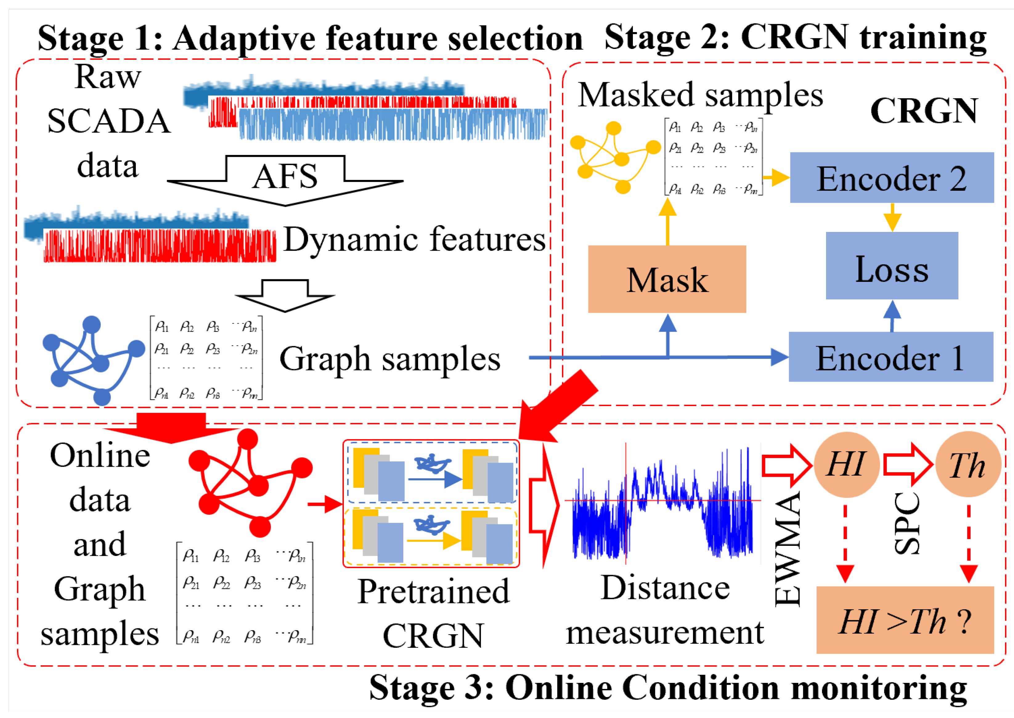
On the basis of the normal behavior model, a WT gearbox condition monitoring method including AFS and CRGN is developed, as shown in Figure 4.
There are three stages in the proposed methodology: adaptive feature selection, CRGN training, and online condition monitoring. Stage 1 consists of data preprocessing and adaptive feature selection. It provides graph data samples for model training in Stage 2 and for condition monitoring in Stage 3. Stage 2 involves deep learning-based training of the CRGN model proposed in this study. It supplies pre-trained models for condition monitoring in Stage 3. Stage 3 is the process of online condition monitoring using samples from Stage 1 and the pre-trained models from Stage 2.
Stage 1: The raw SCADA data is initially preprocessed to eliminate null values and other similar anomalies. Subsequently, features strongly correlated with the wind turbine gearbox are selected based on AFS. A set of selected features is then prepared, dynamically varying according to different wind turbines. Finally, a graph data sample is generated based on feature correlations and the raw data.
Stage 2: After graph data samples are prepared, Gaussian random noise is introduced into the samples to construct a mask for model training. Based on contrastive learning, offline CRGN model training is performed to develop two encoders that share initial weights, each comprising a GNN with residual connections.
Stage 3: The pre-trained model from Stage 2 is integrated into the online monitoring system. Meanwhile, according to Stage 1, graph samples are constructed using online data under unknown operating conditions. Subsequently, the predictions generated via the pre-trained model are compared with those from healthy samples to compute the distances in multi-dimensional space. Based on these distance metrics, HI for the gearbox is constructed in conjunction with EWMA. Finally, the failure threshold Th is established using SPC, and the relative magnitudes of HI and Th are compared to facilitate online CM for the WT gearbox.
The three stages constitute a comprehensive framework for wind turbine gearbox condition monitoring, encompassing various aspects such as data acquisition, data preprocessing, feature selection, graph sample construction, graph neural network-based model training, online data integration and model configuration, similarity measurement, the development of a health index, and the determination of failure thresholds.

3. Application and Discussion for Proposed Method

3.1. Case I: Validation on SCADA Data from a Wind Farm in China

3.1.1. Raw SCADA Data

The data utilized for the application is sourced from specific 3 MW wind turbines and their associated SCADA system deployed within a wind farm in Gansu Province, China. The spatial distribution of the turbines across the farm area is illustrated in the mesoscale satellite distribution map shown in Figure 5a. In Figure 5b,c, there are variations in the power output and wind speed for WT No. 01 and WT No. 03 among the 32 WTs in the wind farm.
The wind farm includes 32 wind turbines. The data comprises 10-min interval measurements for the year 2021, involving 104 features within the SCADA system. According to the O&M reports from the wind farm, various faults have occurred in WTs No. 09, No. 14, No. 25, No. 27, No. 31, and No. 32, as shown in Table 2. The fault discovery time is defined as the moment when technicians identified anomalies such as unusual noises or elevated temperatures during inspection.
The WTs experiencing faults too early, such as WT No. 14 and No. 31, cannot reflect the specific changes in their conditions. In contrast, other WTs can reflect the changes in their operational conditions to varying degrees. More importantly, the available data for the WTs covers the year 2021 only. As for the faulty WTs, there is no access to their early operational healthy history data, which is disadvantageous for model training and CM. Since all 32 WTs in this wind farm are from the same batch and are relatively concentrated in layout, their working environment is relatively consistent. It is thus feasible to validate the method within an allowable margin of error by replacing the early healthy historical data of the faulty WTs with the data of healthy WTs. Therefore, the data of healthy WTs is used for model training, followed by condition recognition and assessment of the faulty units.

3.1.2. Validation of CRGN

Based on AFS, the experimental samples are selected using the graph construction method developed in this paper. They are then input into the preset CRGN for training. Table 3 presents the settings for the fundamental hyperparameters of the model training.
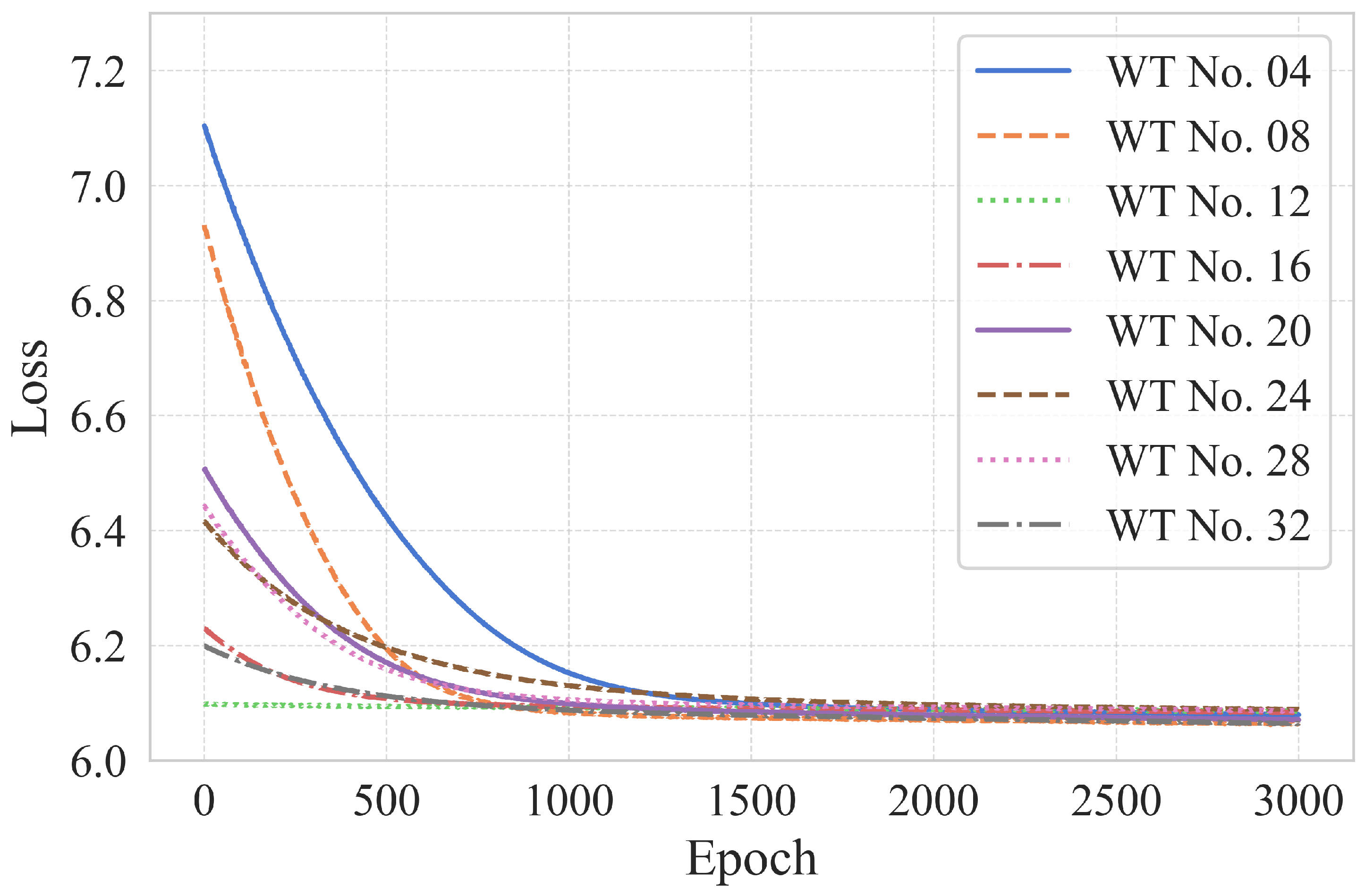
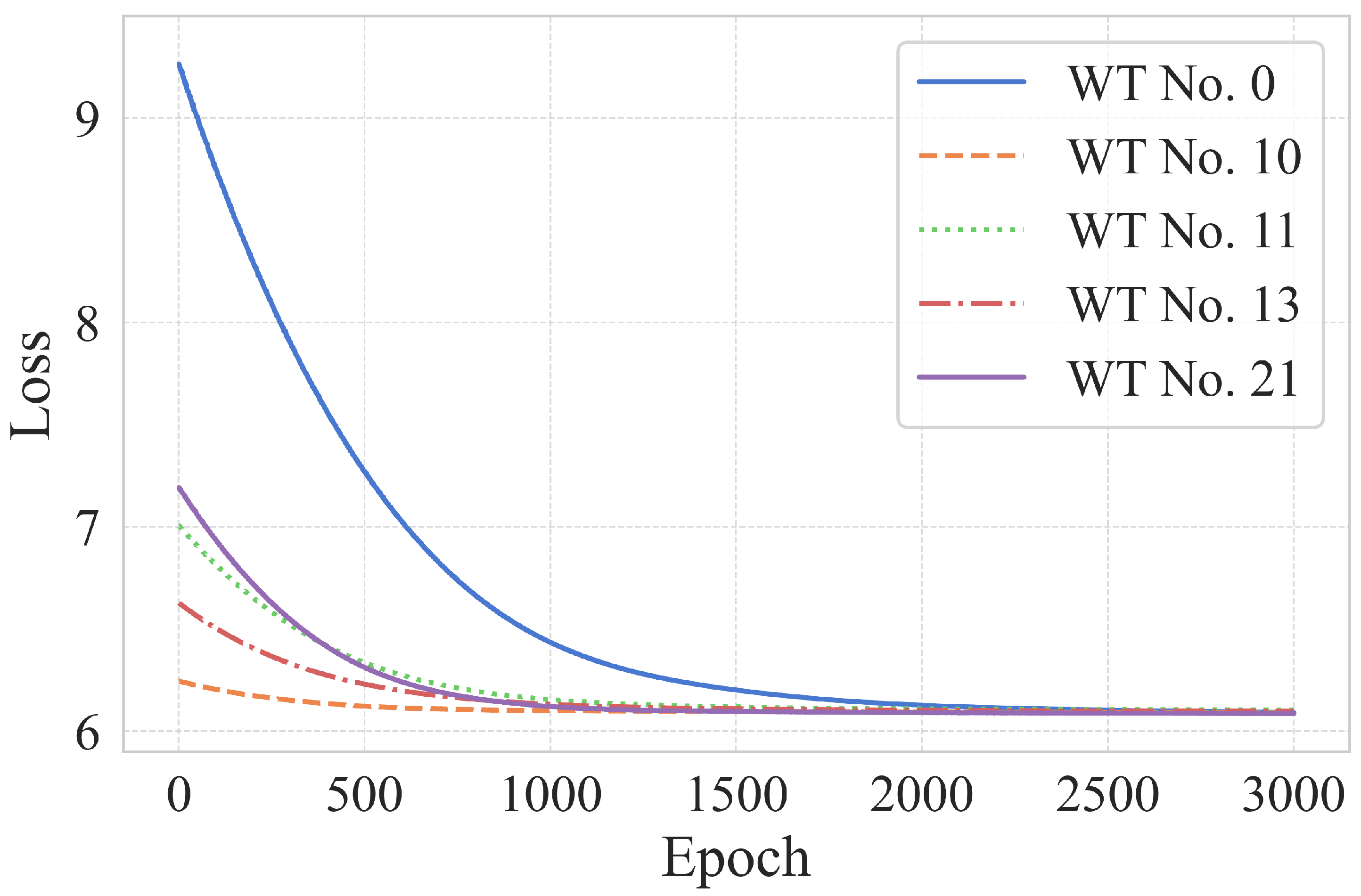
Model training is conducted for all 32 wind turbines within the wind farm. The same data preprocessing and AFS are applied to each turbine. With the recombination of the selected dynamic features, graph data sampling is performed, and model training is subsequently conducted. Figure 6 illustrates the variation in loss values corresponding to the data of several turbines during training. After 1500 epochs, the training process tends to converge. Therefore, the AFS method and the training process of the CRGN proposed in this paper are considered effective.
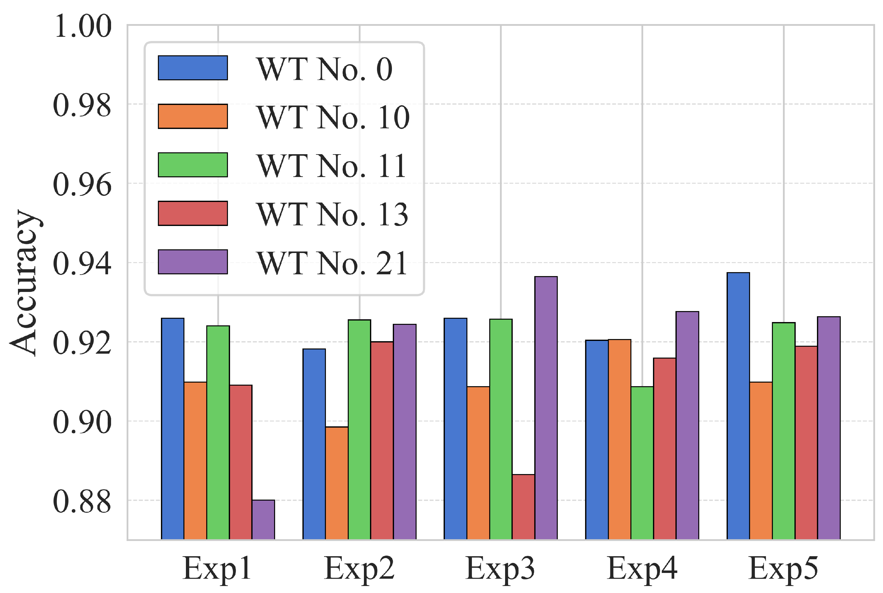
To evaluate the recognition accuracy of the model in the target CM task for WT No. 25 gearbox, experiments are conducted to determine whether the model is applicable to accurately identify the anomalies. Verification is performed by analyzing the time period prior to on-site maintenance personnel detecting the anomaly, with the results shown in Figure 7. To eliminate the interference caused by random factors, different experimental groups Exp 1 to Exp 5 are subjected to the same conditions. The 99% confidence intervals for the results of each experimental group are as follows: (0.8864, 0.9230), (0.8840, 0.9222), (0.8831, 0.9279), (0.8924, 0.9254), and (0.8759, 0.9281).
As is illustrated in the figure, the models trained on data from various wind turbines can attain a recognition accuracy exceeding 90% in the gearbox CM task for WT No. 25, with the experimental results of each group remaining within a limited variance range. Therefore, the AFS and CRGN methods are considered effective in the CM task of gearboxes for WTs.

3.1.3. Validation of Condition Monitoring for WT Gearbox

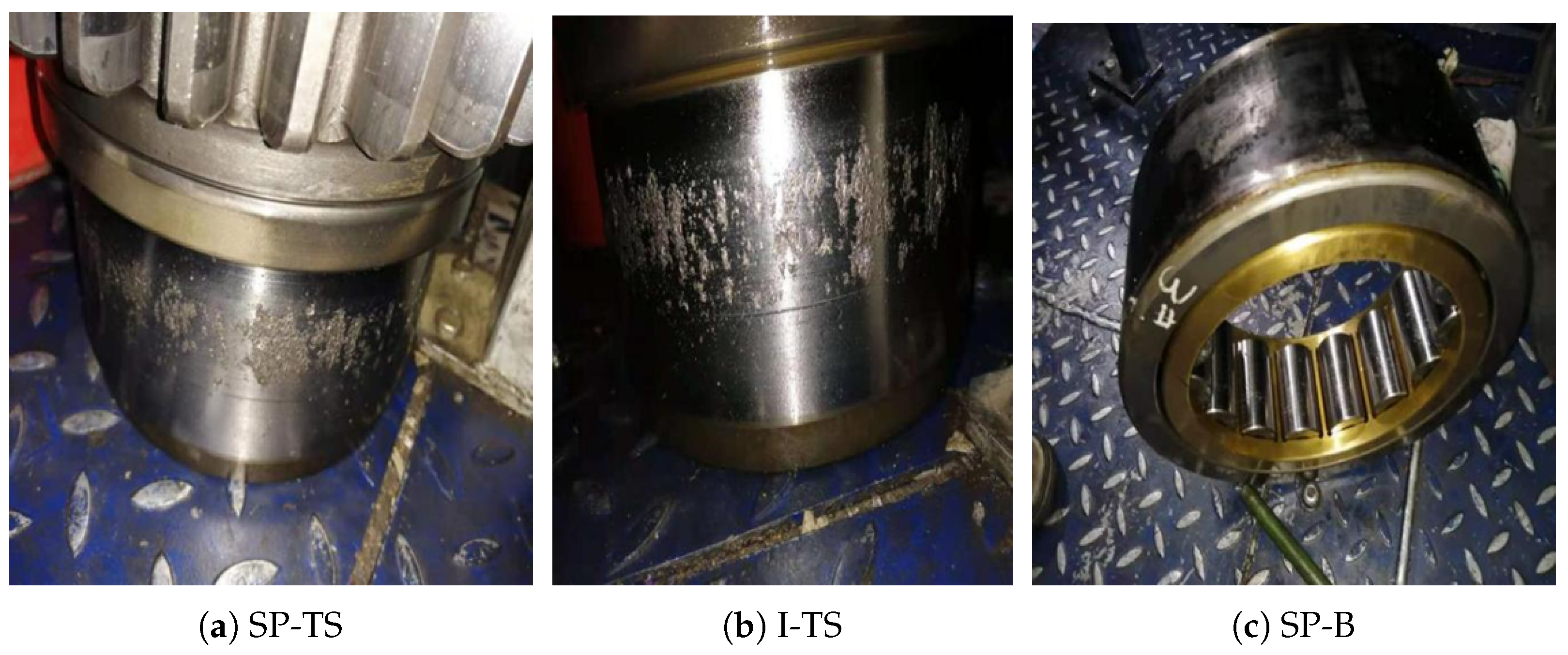
According to the O&M report, an anomaly is detected in WT No. 25 on 28 April 2021. Upon inspection, it is identified as a gearbox failure. Specifically, it manifests as spalling on the high-speed shaft tooth surface (SP-TS), the indentation of the high-speed shaft tooth surface (I-TS), and spalling on the high-speed shaft bearing (SP-B). Figure 8 illustrates such faults occurring with WT No. 25.
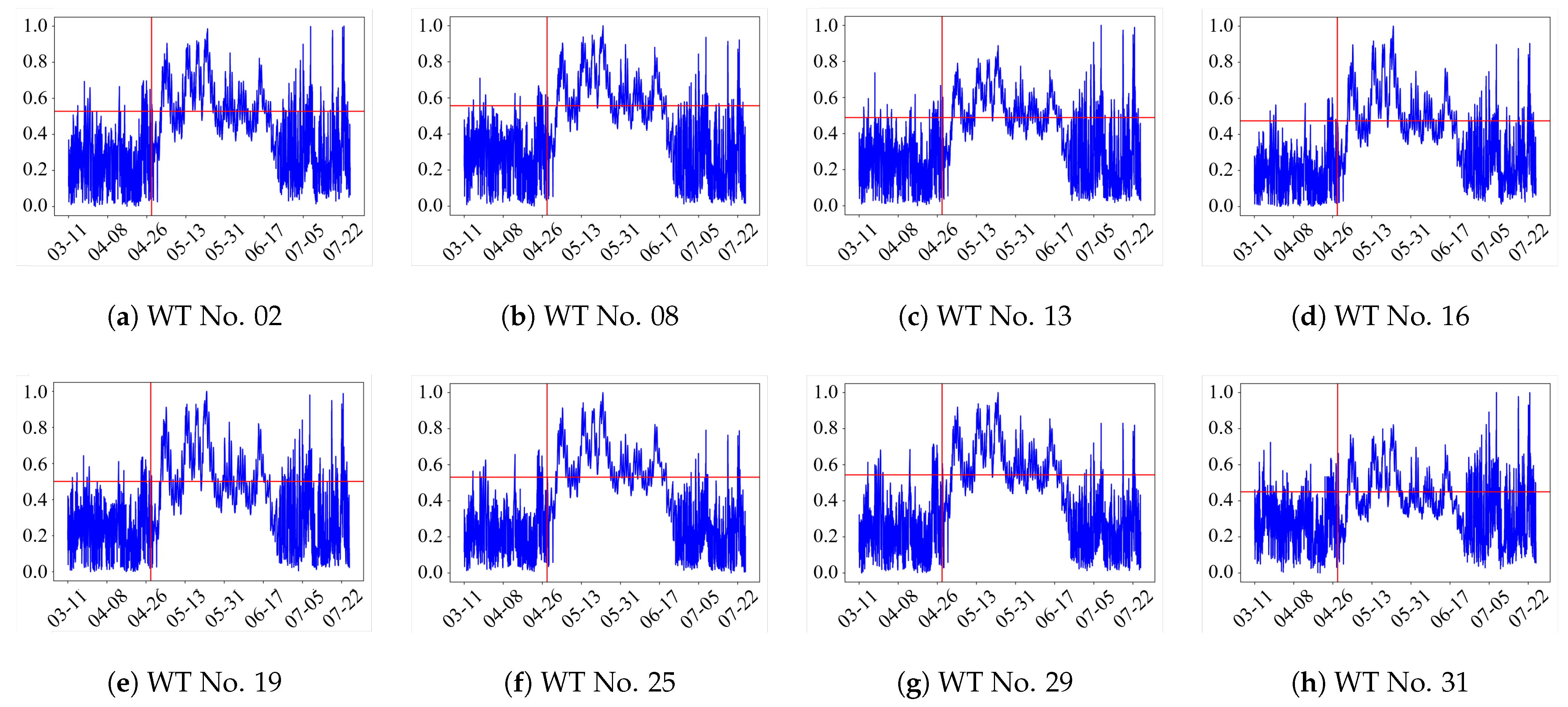
Figure 9 illustrates the distance metrics d a v g between unknown condition data and healthy samples for CM of the gearbox of WT No. 25. The figure depicts the variations in distance metrics during online CM. Different WT numbers indicate that data from various WTs are utilized for model pre-training. The red vertical lines denote the time points at which anomalies were detected, while the horizontal lines represent the recommended reference failure thresholds. Clearly, simple changes in distance metrics are ineffective in identifying the operational condition changes in the WT gearboxes.
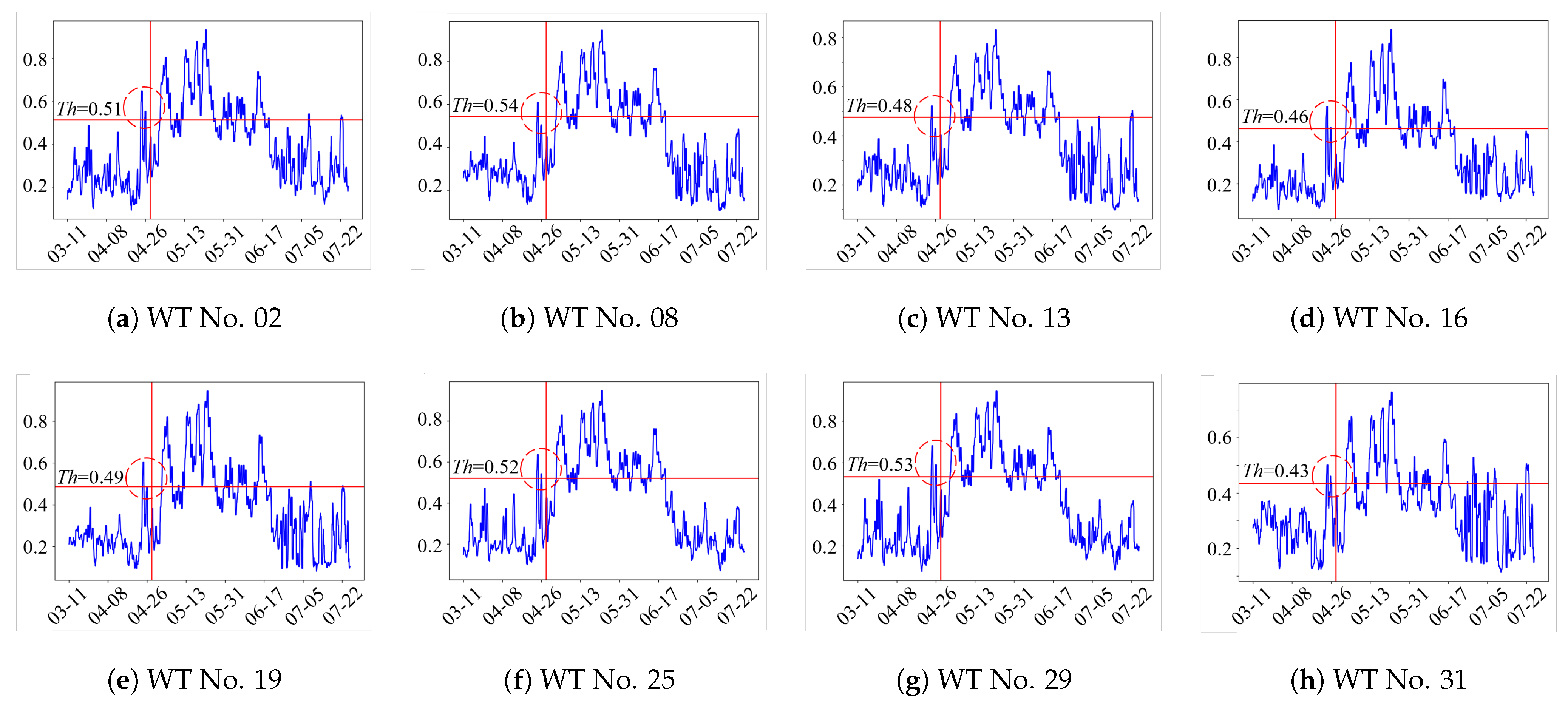
Simply observing the changes in this distance reveals the trend of condition variation, providing a qualitative demonstration of the effectiveness of condition monitoring. For a quantitative perspective, based on the aforementioned distance metric changes, the EWMA and the SPC are applied to establish HI for the changes in operational conditions of the gearbox. Figure 10 shows the HI change, illustrating the condition changes in the gearbox for WT No. 25. Each sub-figure shows that the CM is based on the model pre-trained using data from the corresponding WT. The vertical lines represent the time points at which the anomaly was discovered on-site, while the horizontal lines indicate the failure threshold established under different circumstances. The dashed circles represent that WT anomalies are identified before they are detected by O&M personnel on-site.
Based on the three different types of faults SP-TS, I-TS, and SP-B in the obtained operation and maintenance report, the health guidance constructed in this article has a physical connection with the actual changes in fault status. It can be used to describe the condition changes of the wind turbine gearbox caused by fault changes.
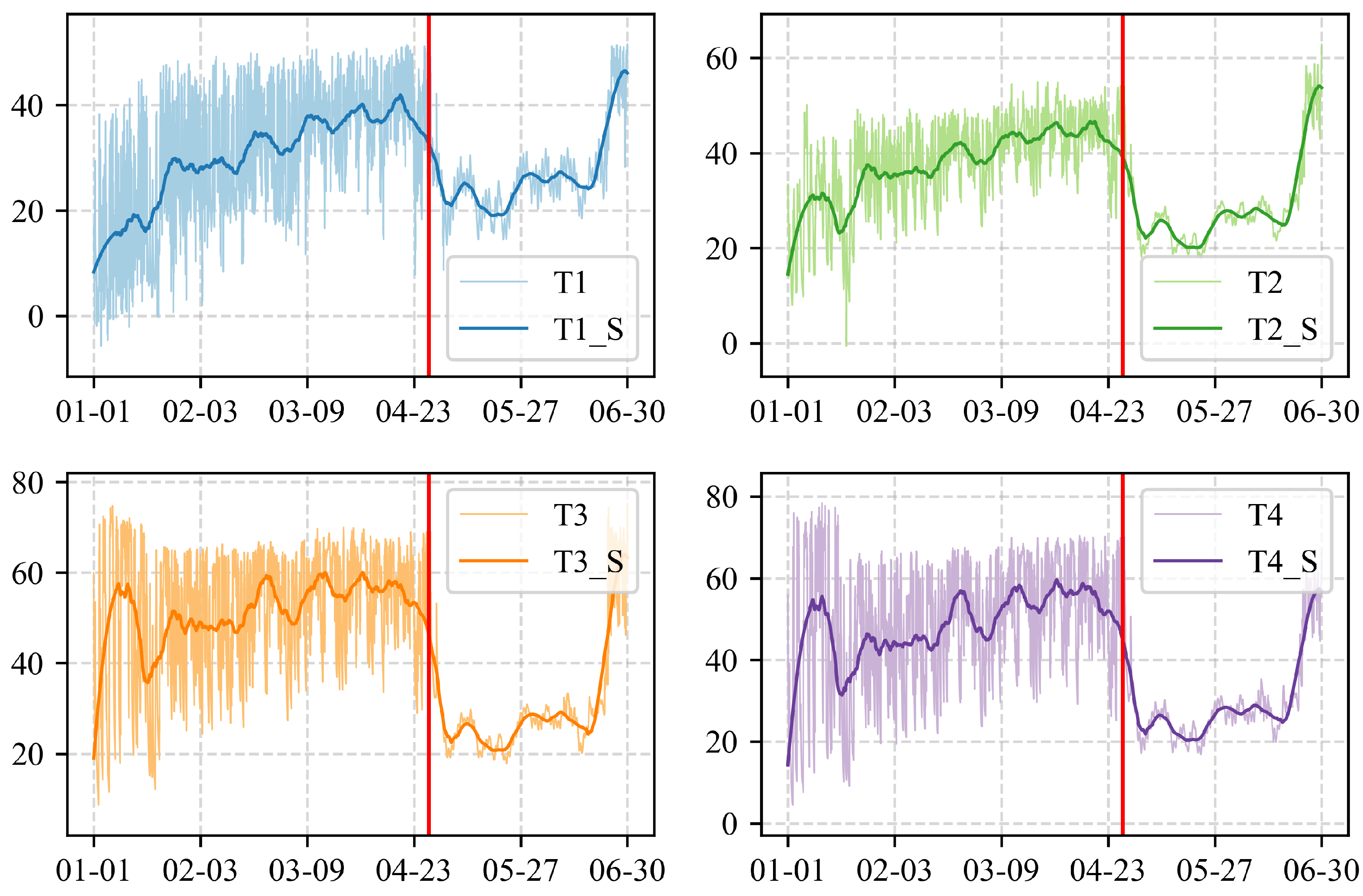
To describe the actual condition change of the WT No.25 gearbox, several temperature parameters related to the gearbox from SCADA data are depicted in Figure 11. The horizontal axis represents time, while the vertical axis represents temperature in degrees Celsius. The red vertical line in the figure indicates the time point when on-site personnel detected an anomaly in the wind turbine. In the figure, T1 is Average oil temperature at gearbox inlet, T2 is the average oil temperature of the gearbox, T3 is the average temperature of gearbox bearing 1, and T4 is the average temperature of gearbox bearing 2. Ti_S ( i = 1 , 2 , 3 , 4 ) indicates that the 2000 pts Savitzky–Golay smooth method is used for several temperature parameters to describe the overall trend of change.
As shown in Figure 11, all temperatures exhibited an upward trend before the gearbox anomaly was detected on site. After the anomaly was identified, the shutdown caused the temperatures to decrease. This indicates that the WT was already operating in an unhealthy condition prior to the failure. The detection results from Figure 10 are consistent with the condition changes illustrated in Figure 11. However, the reasons for not directly analyzing individual SCADA data, but instead employing the method proposed in this paper for CM, are as follows: (1) Wind turbines are equipped with numerous sensors, making it difficult to accurately determine which one to select, and sensor readings often include random errors. (2) Variations in raw sensor signals are not easily observable. The data smoothing applied in Figure 11 serves merely as a tool to illustrate the overall trend, but it sacrifices a significant amount of information contained in the original data. (3) A single sensor provides limited information, whereas the method in this paper integrates signals from multiple sensors, thereby maximizing the extraction of meaningful information from the data. (4) Even when analyzing multiple sensors collectively, it remains challenging to effectively integrate them into a unified framework and to establish consistent health indexes or failure thresholds, which makes practical implementation difficult.
The method proposed in this paper is well suited to overcoming these challenges. According to the O&M report provided by the wind farm, the gearbox of WT No. 25 used for monitoring exhibits various fault types, such as SP-TS, I-TS, and SP-B. For mechanical components that fail, the failures are typically not instantaneous unless extreme wind conditions, external transient shocks, or similar events are encountered. Based on the O&M report and SCADA data, no extreme wind conditions or external transient shocks are observed during the monitored period in this study. Therefore, it can be inferred that the failure of these components results from a cumulative fatigue damage process.
Spalling and indentation are both forms of fatigue-induced crack propagation. It takes time for cracks to grow from the micro level to the macro level. When O&M personnel detect a WT failure at the wind farm, cracks are visible at the macro level. The period prior to this moment is characterized by cracks progressing from micro genesis to propagation and finally to macroscopic manifestation. In this paper, the CM involves accurately identifying changes in the condition of the WT gearbox and analyzing the data in depth to extract anomalous information ahead of the occurrence of macroscopic cracks.
Figure 10 illustrates the fault development process. According to the sub-figures, the proposed CM method effectively identifies the time interval of anomalies in the WT gearbox. It accurately reflects changes in abnormal conditions during operation and provides a dynamic failure threshold within a reasonable range based on differences in the model training process. Clearly, the method presented in this paper is effective for the condition monitoring of WT gearboxes.
The HI in each sub-figure exhibits a downward trend when abnormal information is identified, which aligns with the actual operation of wind turbines. As it takes a certain amount of time for microscopic anomalies to develop into macroscopic anomalies, the condition changes, and a downward trend is observed. The models pretrained using different wind turbine data exhibit the same trend in the condition monitoring results for WT No. 25 gearbox, which implies the effectiveness and consistency of the method proposed in this paper. Regarding the completion time of wind turbine maintenance, the condition of the gearbox returns to below the failure threshold. Despite the less-than-satisfactory performance achieved on some pretrained models of the wind turbines, a unified overall trend of change is observable. Therefore, the adaptive condition monitoring method proposed in this study is considered applicable to produce satisfactory results in the condition monitoring task of wind turbine gearboxes and effective for identifying condition changes from normal to abnormal before returning to normal during wind turbine operation.
For practical application, anomaly information recognized in advance can be transmitted to the control system of a wind turbine. Along with regulating the turbine’s orientation and operational process, this information can prevent or delay subsequent macroscopic failures, thereby extending the turbine’s effective operational lifespan. In this context, the detection of micro-anomalies shortly before the occurrence of macro-anomalies can be regarded as valuable operational and maintenance insight, indicating effective early recognition within a specific threshold.
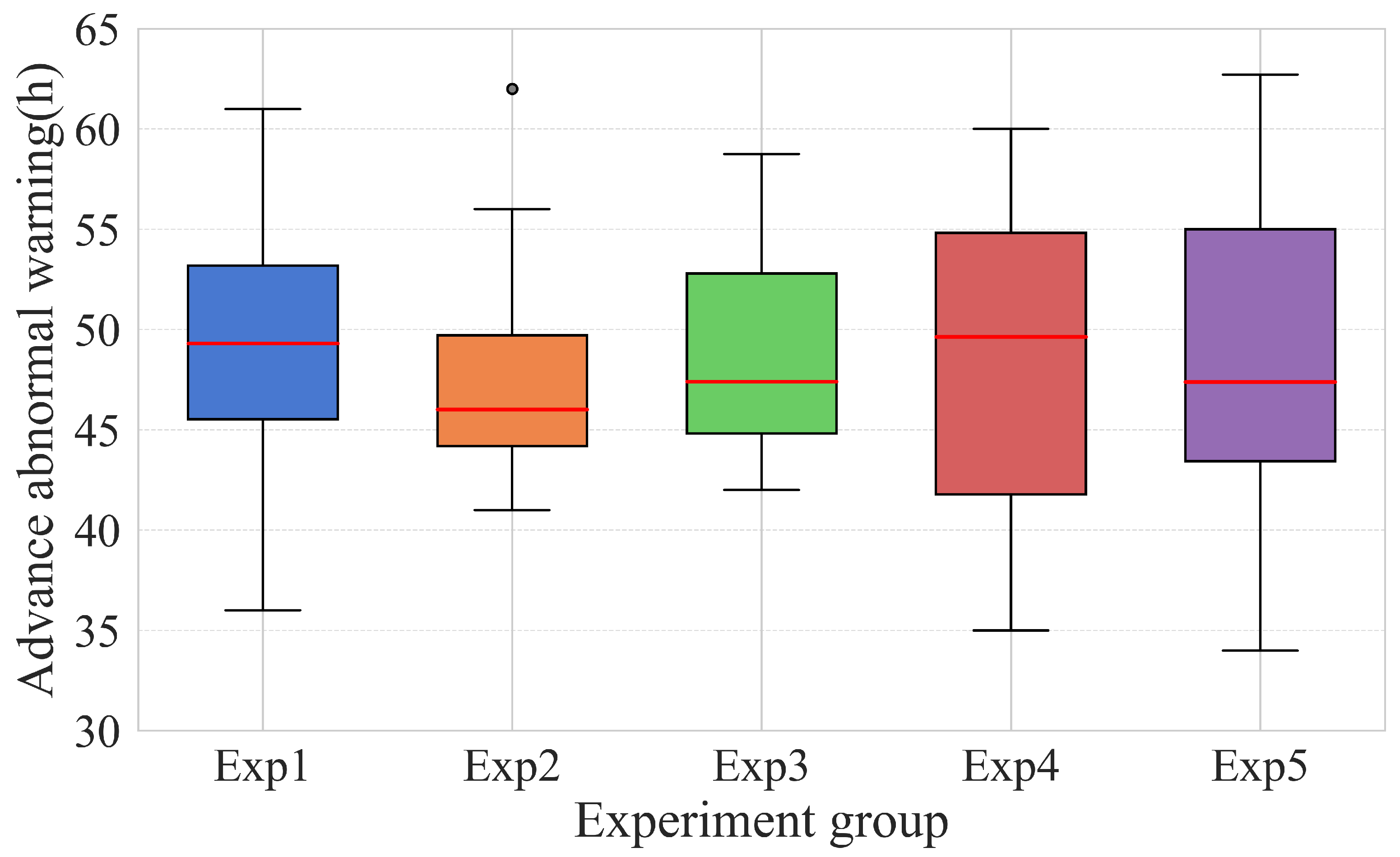
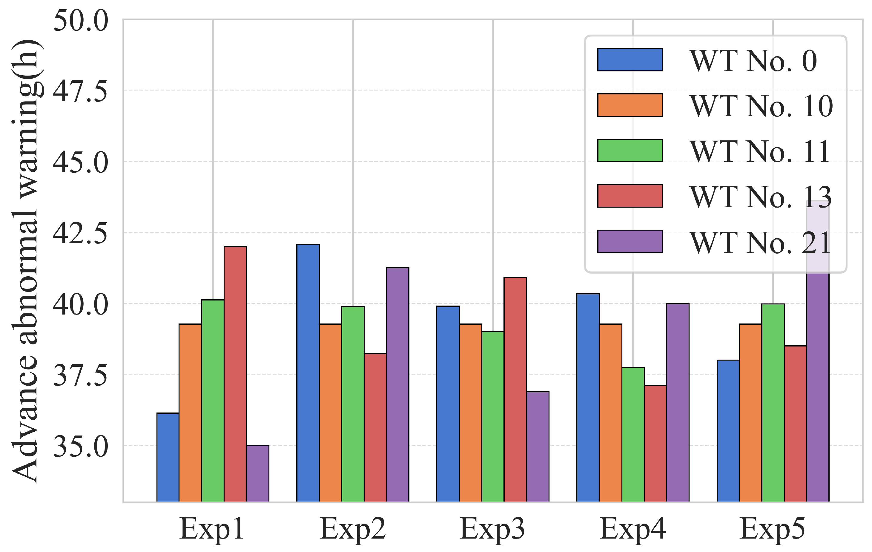
Furthermore, this method can be used to issue early warnings of WT gearbox failures. That is to say that the HI exceeds the failure threshold for a period of time before anomalies are detected on-site, and it represents a sustained signal, rather than a transient one. Statistically, the advance warning of anomalies for the WT No. 25 gearbox can achieve a lead time of 30–40 h under the above scenarios. To determine whether this phenomenon is random, five similar experimental groups, Exp 1 to Exp 5, are conducted under the same settings. The 99% confidence intervals for the results of each experimental group are as follows: (44.73, 51.67), (45.00, 50.26), (46.27, 50.91), (43.78, 52.66), and (43.97, 50.60). The box plot in Figure 12 shows the time of advance warnings for the gearbox of WT No. 25, based on pre-trained models with data collected from different WTs.
The average advance warning time for gearbox abnormality identification in WT No. 25 ranges between 46 and 49 h. Excluding certain interference factors, it is evident that the method presented in this paper is applicable for extracting abnormal information from the raw SCADA data of wind turbines, monitoring gearbox operation, and detecting microscopic abnormal signals prior to failure. Consequently, an early warning can be issued. With a lead time exceeding 40 h, sufficient time is available for the wind farm to inspect the potentially faulty gearbox. This not only prevents the progression of the fault but also mitigates greater losses and subsequent chain failures of the wind turbine caused by gearbox failure, thereby avoiding cascade effects.

3.1.4. Compare to Other Methods

To validate the superiority of the proposed method, a set of methods are organized for comparison. The methods with some specific information are as follows.
  • Baseline: unsupervised autoencoder (UAE) with 2 layers in the encoder. The input, hidden, and output channels are (16, 32, 32) in encoder. The objective function used for training is the root mean square error.
  • Support vector machine (SVM) with 32 SVM regressors.
  • Convolutional neural network (CNN) with 2 convolution layers. The input and output channels of each layer are (1, 64) and (64, 128), respectively.
  • Long short-term memory (LSTM) with 1 layer. The input, hidden, and output channels are (40, 32, 32), respectively.
  • Local outlier factor (LOF) with neighbors number k = 20 .
  • Isolation forest (IF) with 128 trees.
  • Transformer (TSFM) with 2 transformer Layers. The input, hidden, and output channels of each layer are (40, 32, 32), respectively.
  • Deep belief network (DBN) with 2 layers of restricted Boltzmann machines. The input, hidden layer, and output layer channels are (40, 32, 32).
  • Traditional graph neural network (TRAGNN) with 2 graph convolutional network layers. The input and output channels of each layer are (40, 32) and (32, 32), respectively.
  • The proposed self-supervised contrastive residual graph neural network (CRGN).
The basic hyperparameter settings for different methods are similar to those proposed in this paper. Upon comparison, six metrics are used: recognition accuracy (M1), F1-score for recognition (M2), advance anomaly warning time (M3), model operating time (M4), the trainable model parameter quantity (M5), and the effectiveness of condition monitoring (M6). M1, M2, and M3 are used to verify the performance of the model and the condition monitoring results. M4 represents the online inference time, and M5 represents the computational complexity and memory usage. M6 is a qualitative indicator used to evaluate the condition monitoring performance of the target task. It is determined via the anomaly recognition and condition monitoring results. The performance of the various methods is shown in Table 4.
In the table, “Almost none” indicates that the advance anomaly warning time is less than 3 h, while “Few” refers to a lead time of less than 8 h. Based on O&M reports and historical experience, such short warning times are considered unreliable and cannot be regarded as indicators of effective performance. Therefore, the labels “Almost none” and “Few” are used here to reflect the model’s relatively limited effectiveness in these cases.
As shown, the proposed method demonstrates clear advantages in the task of WT gearbox CM. It excels not only in anomaly detection accuracy and advance warning time but also performs favorably in model operating time and parameter count. CRGN has achieved better results than other methods for the condition monitoring task in this paper, which represents the primary objective of this study. It may not surpass deep learning approaches such as CNN, LSTM, TSFM, and TRAGNN in model complexity or operating efficiency, it still ranks at an upper-mid level in these aspects. The operating time and model size are above average, which remains an acceptable outcome. It can be optimized in future work, as the deployment and application of edge computing or PLC systems in the future require lightweight and fast computing methods, which will also be the direction of our efforts.
The baseline adopts a traditional unsupervised autoencoder, and the training objective is to minimize the difference between the original data and the reconstructed data. Due to the neglect of correlations between different features of the original data during training and the use of only the original data, a certain model effect is achieved, but it is not satisfactory.
Compared with traditional machine learning methods such as SVM, LOF, and IF, the proposed method delivers significantly better CM performance, particularly in terms of recognition accuracy and the timeliness of advance warnings. This improvement is mainly because traditional methods cannot deeply extract useful information from large datasets, as they focus on some local information and ignore the correlations between various features.
As a traditional deep convolutional model, CNN performs well in image-processing tasks. However, in the condition-monitoring task presented in this paper, it fails to capture the correlations among different features and instead relies solely on raw data for training. Consequently, its performance is limited and falls short of achieving optimal results.
LSTM can enhance model performance by considering temporal sequences information. However, similar to the limitations of CNN, it cannot effectively capture correlations among different features, which leads to suboptimal performance.
TSFM generally outperforms CNN and LSTM in terms of overall performance. In the CM task presented in this paper, its results are the closest to those of the proposed CRGN method. However, due to its large number of parameters and lengthy operating time, TSFM incurs higher computational costs and greater model complexity. This makes it less favorable for real-world applications where cost control is critical, as it contradicts the primary goal of operation and maintenance work—reducing costs while improving efficiency.
DBN aims to preserve the characteristics of the original features while reducing the dimensionality of the features. Due to the further dimensionality reduction, the hidden feature information contained in the original data becomes diluted. In addition, the training samples are directly taken from the original data, ignoring the correlation among different features. Therefore, the performance in the wind turbine gearbox condition monitoring task is inferior to the method proposed in this paper.
TRAGNN and CRGN share a common foundational framework, but their key difference lies in architectural design. TRAGNN constructs the model using a pipeline based solely on graph convolutional networks, whereas CRGN is developed within a contrastive learning framework and incorporates residual connections. This enables CRGN to effectively integrate raw data, feature correlations, residuals, and contrastive loss during training. As a result, although TRAGNN achieves performance close to that of CRGN in the CM task presented in this paper, it still falls short of matching CRGN’s overall effectiveness.
Overall, the proposed method is effective and demonstrably superior to other methods.

3.1.5. Validation of AFS

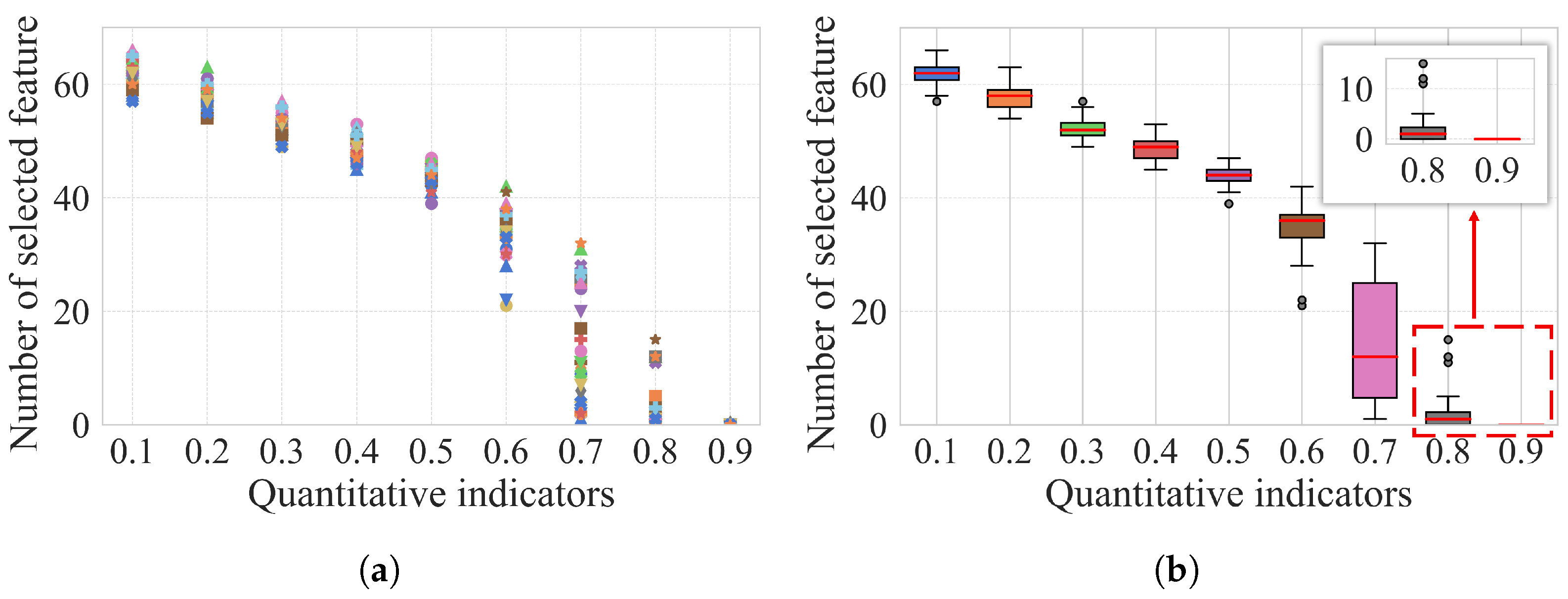
To determine the quantitative indicator in AFS, the results of varying feature selection counts are statistically analyzed, as shown in Figure 13. In panel (a), different markers represent data from different WTs. However, these markers are difficult to distinguish. Since the primary focus is on the range of value changes, specific labels are, therefore, omitted. Notably, the number of adaptively selected features remains relatively stable and high when the quantitative indicator is less than or equal to 0.5, resulting in information redundancy. When the indicator reaches or exceeds 0.7, the feature selection results for some WTs approach zero, making modeling and analysis impossible.
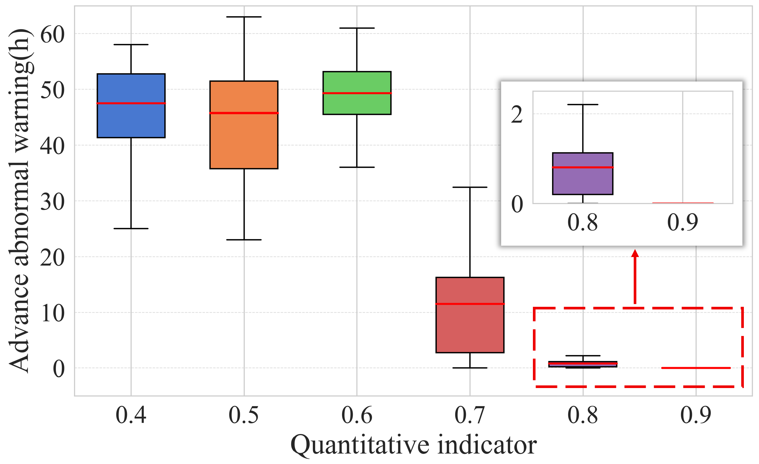
It is essential to examine the impact of various quantitative indicators on CM results. Therefore, different quantitative indicators are used to statistically analyze the advance warning time for abnormalities in the gearbox of WT No. 25, as shown in Figure 14.
The 99% confidence intervals for the results of each experimental group are as follows: (42.13, 50.35), (39.93, 49.29), (44.73, 51.67), (6.47, 15.07), (0.53, 1.17), and (0, 0). When the quantitative indicator is set to 0.4 or 0.5, more features are selected, providing more comprehensive information in the data. However, this also introduces greater uncertainty, leading to poorer performance when data collected from certain wind turbines is used for model training and CM. As a result, the overall distribution range widens, and system operation becomes less stable compared to when the indicator is set to 0.6. Conversely, setting the indicator to 0.7, 0.8, or 0.9 results in selecting fewer features, which limits the information available in the data. This insufficiency hinders model training and CM, increasing the likelihood of underfitting. Therefore, setting the quantitative indicator to 0.6 is more appropriate.
For the raw SCADA data of 32 WTs in the wind farm, the AFS is applied for feature selection. With the quantification indicator set to 0.6, five core features are initially identified in Table 1 with F1–F5. Figure 15 shows the results (number of selected features) of AFS.
Moreover, when the number of core features is reduced from 5 to 3, only features F1 to F3 yield the same results, as illustrated in Figure 15. This indicates that the AFS leads to dynamic changes in the number of data nodes in the graph, and the core features selected for the gearbox CM task in this study are representative of the gearbox. Additionally, for the operational data of different WTs, a specific subset of feature variables can be accurately and adaptively selected for subsequent model training and validation.
To validate the AFS, a comparative experiment is conducted on the following groups: no feature selection (No FS), AFS, the use of only core features (5 core features and 3 core features), as shown in Table 5.
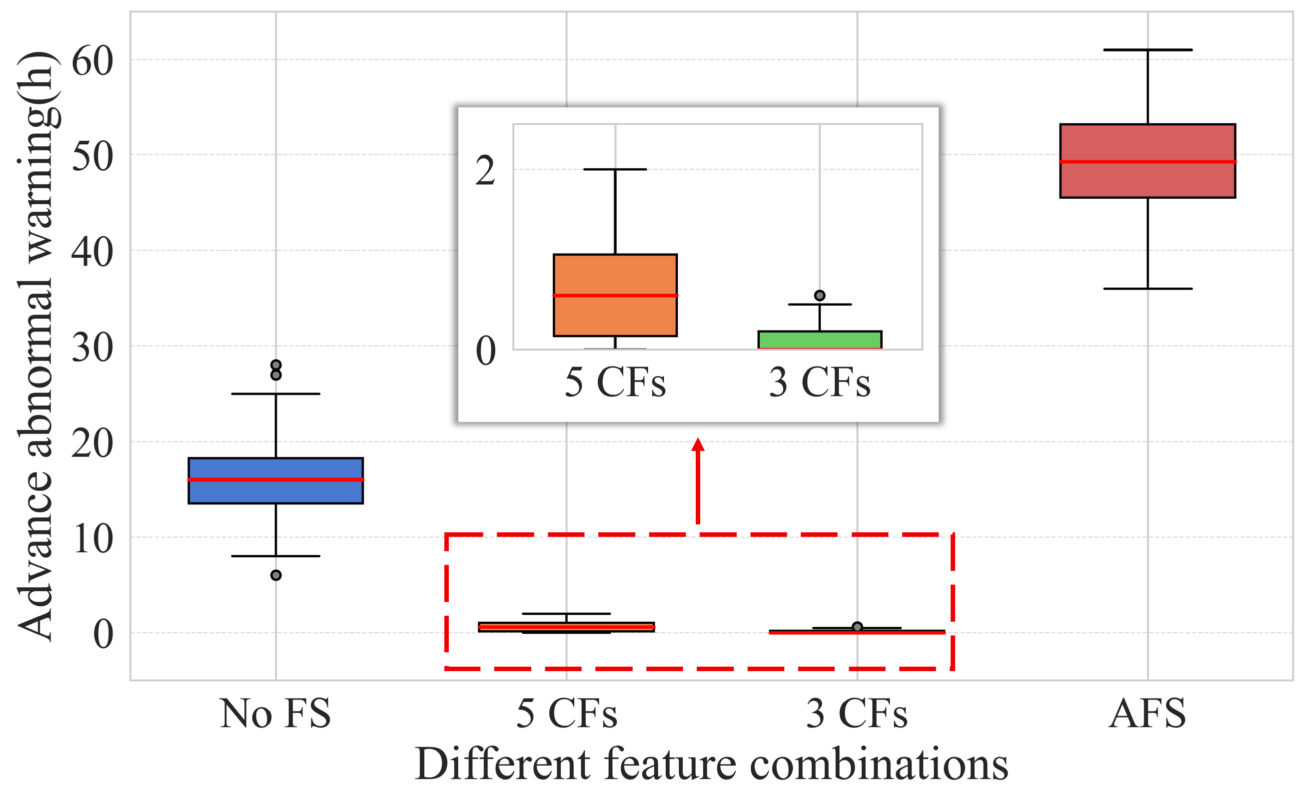
Figure 16 presents the experimental results obtained about the advance warning lead time for the abnormality of the gearbox of WT No. 25.
The 99% confidence intervals for the results of each experimental group are as follows: (13.63, 18.89), (0.44, 1.08), (0.04, 0.20), and (44.73, 51.67). When No FS is performed, there is a great redundancy introduced via the use of all 104 features, which affects the model training and CM results adversely. On the other hand, the model is underfitted due to insufficient information when only some core features are used for model training, which leads to an almost zero advance warning lead time for anomalies. Therefore, the AFS proposed in this paper is deemed effective and practical.

3.1.6. Validation of Failure Threshold

In Section 2.4, a failure threshold based on SPC is defined where the threshold coefficient value v = 2.326 . However, some related studies have employed alternative values such as 2, 3, 4, and 5. Therefore, in this section, a series of validation experiments is conducted. Based on the concept of the normal distribution, the probabilities of the quality characteristics falling within the ranges of ( , μ + 2 σ ] , ( , μ + 3 σ ] , ( , μ + 4 σ ] , and ( , μ + 5 σ ] are 0.97724987, 0.99865010, 0.99996833, and 0.99999971, respectively. As mentioned earlier, drawing on historical experience, and to ensure the generalization of our method, we have selected a confidence level of 0.99, which corresponds to the value of 2.326.
In the context of the condition monitoring task discussed in this article, various numerical values, v, influence the determination of the ultimate failure threshold, which in turn affects the outcomes of online condition monitoring. These effects are mainly reflected in three aspects: the feasibility of achieving condition monitoring, the lead time for early warnings, and the accuracy of anomaly detection. To verify the impact of different values on the results, a series of supplementary experiments is conducted.
Six metrics are defined to compare the influence of different values of v on the results of CM, named confidence level (IR1) when calculated with the probabilities of the quality characteristics falling within various ranges, threshold (IR2) calculated with different v, anomaly recognition accuracy (IR3), advance time for abnormal warning (IR4), effectiveness of CM (IR5), and the possibility of mistake alarm (IR6). Among them, IR5 and IR6 are qualitatively assessed based on the practical performance of condition monitoring, whereas the others are quantitatively evaluated. Experimental results are presented in Table 6, showing the condition monitoring results for WT No. 25 gearbox with the pre-trained model trained by data from WT No. 01.
From the table, we observe that the failure threshold increases as v increases, as does the confidence level. However, the recognition accuracy initially decreases and then rises, reaching 100% when v = 4 and 5. This occurs because, within a reasonable range of v, the health index is negatively correlated with v. When v exceeds this range, the model and algorithm become inefficient, resulting in an accuracy of 100%, which indicates a mistake in condition monitoring. A similar pattern is observed for the advance warning time for abnormalities: it shows a negative correlation with v within a specific range, but significant errors arise when v goes beyond this range. Considering both the effectiveness of condition monitoring and the likelihood of false alarms, v = 2.326 performs better than other values.
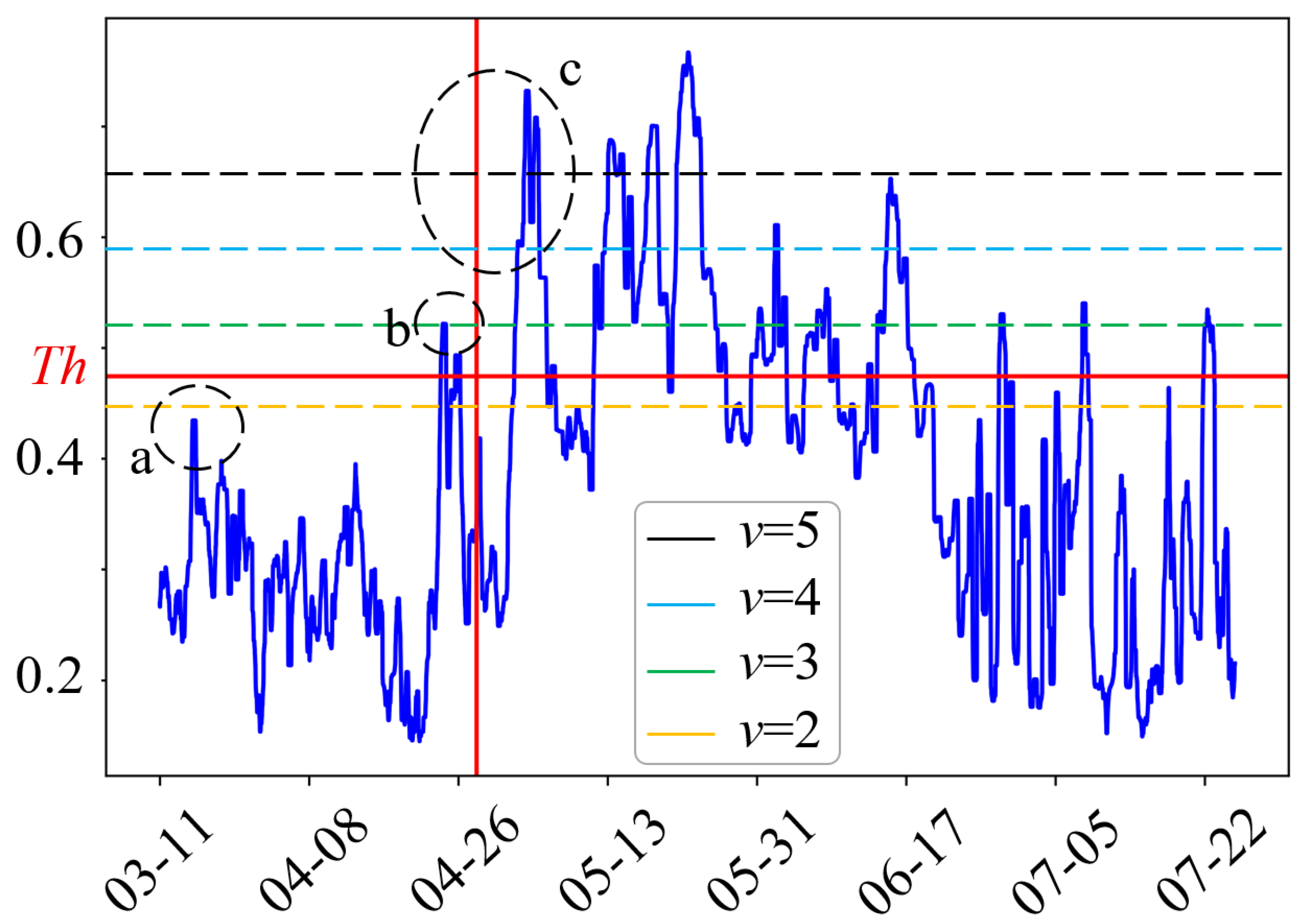
Different thresholds can be calculated based on various v. The condition monitoring results for WT No. 25 gearbox with the pre-trained model trained by data from WT No. 01 are presented separately, with a comparison of the different thresholds shown in Figure 17.
In the figure, at position a, the low confidence level leads to a scarcity of effective information in the quality control process and a heightened risk of false positives during condition monitoring. Position b experiences weak condition monitoring, resulting in low accuracy in effective condition recognition. Meanwhile, position c lacks any abnormal warnings and exhibits noticeable errors in its condition monitoring results.
Therefore, the specific value v is suitable to be 2.326 in the task of CM for WT gearbox.

3.2. Case II: Validation on SCADA Data from a Wind Farm in Portugal

3.2.1. Raw Data Expression and Validating Preparation

In order to verify the generalization ability and robustness of the proposed method under different working environments, wind turbines, and their operating conditions, another dataset is selected to validate the proposed method on the task of wind turbine gearbox condition monitoring. The second dataset [47] comprises data from three wind farms. The dataset from Wind Farm A, which includes 5 wind turbines from an onshore wind farm in Portugal, is used for validation. Wind Farm A contains 22 sub-datasets, with 10 representing normal conditions and 12 representing abnormal conditions. Each sub-dataset consists of data from 54 sensors, corresponding to 86 features. Some of these features include the maximum, minimum, average, and standard deviation values of the respective sensors. The sampling interval between data is 10 min and the data covers the period from 2022 to 2023. The recorded faults are listed in Table 7.
According to the description of dataset and wind farm, WT No. 21 with a gearbox failure is selected as the CM target. Based on analysis of sensors and features, 3 core features are selected for AFS, called Temperature in gearbox bearing on high speed shaft, Temperature oil in gearbox, and Generator rpm in latest period, corresponding to sensor_11_avg, sensor_12_avg, and sensor_18_avg, respectively. They describe the temperature and rotational speed of the gearbox, being the most correlated features to gearbox. Hyper-parameters for model training and condition monitoring refer to those in the previous validation.

3.2.2. Validation of CRGN

Normal data from each wind turbine is used for CRGN model training. The training loss of five WTs can be seen in Figure 18. It can be observed that the training tends to converge after 1500 epochs, illustrating that CRGN proposed in this paper is efficient in the 2nd dataset.
The recognition accuracy of the model for the target CM task on the WT No. 21 gearbox is shown in Figure 19. Five groups of experiments are presented. Different WT numbers indicate models trained using data from the corresponding wind turbines. It can be observed that the recognition accuracy of the various models averages above 90%, which is comparable to the results obtained in the previous validation in Case I. Therefore, the validation of the CRGN proposed in this paper is effective and demonstrates good generalization.

3.2.3. Validation of Condition Monitoring for WT Gearbox

According to the description of the dataset, gearbox failure of WT No. 21 begins at the moment 10 October 2023 08:40, and ends at 17 October 2023 08:40. The CM validation primarily takes place within this period. Figure 20 illustrates the HI changes of the gearbox in WT No. 21, with each sub-figure corresponding to the models trained using data from different WTs. The vertical lines indicate the time points at which anomalies begin, while the horizontal lines represent the failure thresholds established under various conditions. The Th labels in the sub-figures denote the failure threshold values for each condition monitoring task. The dashed circles highlight instances where WT anomalies are detected at the macro level before being observed on-site.
The figure illustrates the evolution of the HI for the gearbox of WT No. 21. Following the recorded onset of the anomaly, the HI exhibits considerable fluctuations. Notably, the HI clearly exceeds the failure threshold before the recorded anomaly begins. This indicates that the condition monitoring for the WT No. 21 gearbox is effective. Furthermore, when the models are trained using healthy data from different turbines and then applied to monitor the condition of the WT No. 21 gearbox, the HI demonstrates a consistent developmental trend across different models. This suggests that the proposed method exhibits strong adaptability and generalization ability on this dataset.
Additionally, an important function of condition monitoring is to provide early anomaly warnings. This enables maintenance personnel to receive predictions of future anomalies during turbine operation in real-world applications, ensuring sufficient time for intervention and corrective actions. In this validation, the results of the early anomaly warning over the time period are shown in Figure 21. It can be observed that, among five groups of experiments, the average early warning time is approximately 40 h, indicating that the proposed method performs well in condition monitoring on this dataset.

3.2.4. Compare to Other Methods on 2-nd Dataset

To validate the superiority of the proposed method on the 2-nd dataset, a set of methods are organized for comparison, including UAE, SVM, CNN, LSTM, LOF, IF, TSFM, DBN, TRAGNN, and the proposed CRGN model. The basic frameworks of such methods refer to those mentioned in Section 3.1.4. Six metrics are used for validation: recognition accuracy (M1), F1-score for recognition (M2), advance anomaly warning time (M3), model operating time (M4) and trainable model parameters quantity (M5), effectiveness of condition monitoring (M6). The hyper-parameters settings of each method are similar to those of CRGN. Various methods performance can be seen in Table 8, with all the values being average among several experiments.
Similar to Case I, “Almost none” indicates that the advance anomaly warning time is less than 3 h, while “Few” refers to a lead time less than 8 h. Such short times are considered unreliable and should not be regarded as indicators of effective performance.
As shown in the table, the CRGN in this article is above average in terms of model operating time and model size, and it consistently outperforms the other methods in the same condition monitoring task. The baseline UAE lacks consideration for the correlation between data features, so it cannot achieve satisfactory performance. Traditional machine learning methods such as SVM, LOF, and IF are limited in their ability to extract deep information from data, resulting in weak monitoring performance characterized by unsatisfactory anomaly detection accuracy and short advance warning times. CNN also yields poor results in this context, primarily because it fails to consider the temporal dependencies of the raw data and the correlations among different features—factors critical to effective condition monitoring. In contrast, LSTM performs better due to its ability to capture temporal dependencies during training. The further dimensionality reduction of DBN reduces data sensitivity and ignores the correlation between features, resulting in poor model performance. Both TSFM and TRAGNN demonstrate strong performance. TSFM benefits from the application of self-attention mechanisms, while TRAGNN gains an advantage by capturing correlations among different features of the raw data. However, CRGN surpasses TRAGNN by incorporating contrastive learning and residual connections, which effectively reduce uncertainty and enhance model performance. This provides CRGN with a notable advantage in advance warning time within the condition monitoring task.
Similar results are obtained between the two datasets. The method proposed in this paper can demonstrate satisfactory condition monitoring performance in different working environments, wind turbines, and operating conditions, illustrating that the method proposed in this paper is effective and with good generalization.

4. Conclusions

A novel condition monitoring framework for wind turbine gearbox based on adaptive feature selection and self-supervised contrastive residual graph neural network (AFS-CRGN) is proposed, including AFS for data preparation, CRGN for model training, HI, and failure threshold for online CM. Validation using SCADA data from two wind farms in China and Portugal demonstrates that AFS enhances monitoring efficiency and reliability, while CRGN exhibits strong generalizability across different turbines and consistently delivers satisfactory performance. For gearbox anomaly detection, the framework enables effective condition monitoring and early warning of abnormalities. The accuracy and F1 score of abnormal condition identification both exceed 90%, indicating the effectiveness of the method proposed in this article and the consistency of the data samples. And the lead time for anomaly detection and warning before a fault occurs can reach 30 to 40 h. Compared to other methods applied to the two datasets, the proposed approach shows superior performance and improved generalization.
Directly predicting anomalies in WT gearboxes in advance using simple sensor signals is challenging. However, intelligent methods remain effective for categorizing abnormal conditions into distinct patterns and extracting deep data insights through pattern recognition. In this paper, based on the correlations among various data features, the proposed CRGN model evaluates the descriptive contribution of each feature to the gearbox condition. By constructing graph samples and adjacency matrices for training, the residual connections enhance the model’s expressive power and generalizability. Additionally, adaptive model training is achieved through contrastive learning, enabling self-supervised tasks on unsupervised data. Furthermore, the established quantified HI is more adaptive to variations among different data features, mitigating randomness in CM, supporting abnormality assessment, and facilitating abnormality detection and early warning.
The limitation lies in the requirement for a large amount of data and generalization in the application of methods for different wind turbines and operating conditions. In addition, we have found that the decline modes of the main shaft bearing and generator follow a pattern similar to that of gearbox. Therefore, such similar degradation trends suggest the method’s potential for extension to other subsystems in future research. At the same time, to apply the method in industrial real-world scenarios, improving computational efficiency and reducing computational costs while maintaining excellent condition monitoring performance will also be an objective of future efforts.
Author Contributions

Conceptualization, W.Y. and M.Z.; methodology, W.Y.; software, W.Y.; validation, W.Y. and J.Y.; formal analysis, W.Y., M.Z., and J.Y.; investigation, M.Z.; resources, M.Z.; data curation, W.Y. and M.Z.; writing—original draft preparation, W.Y. and M.Z.; writing—review and editing, W.Y. and J.Y.; visualization, W.Y.; supervision, M.Z.; project administration, M.Z. and J.Y.; funding acquisition, M.Z. All authors have read and agreed to the published version of the manuscript.

Funding

This research was funded by the National Key Research and Development Program of China (Grant No. 2022YFB4201200), the Key Projects of Stable Funding Support for Universities in Shenzhen (Grant No. GXWD20220817140906007), and Guangdong Basic and Applied Basic Research Foundation (Grant No. 2024B1515250004).

Data Availability Statement

The original data of the paper is currently confidential. Further inquiries can be directed to the corresponding author.

Acknowledgments

We would like to express our sincere gratitude to these funding organizations.

Conflicts of Interest

The authors declare no conflict of interest.

References

  1. Chatterjee, J.; Dethlefs, N. Scientometric review of artificial intelligence for operations & maintenance of wind turbines: The past, present and future. Renew. Sustain. Energy Rev. 2021, 144, 111051. [Google Scholar] [CrossRef]
  2. Yang, H.; Jiang, X.; Zhao, H.; Wang, Z.; Cheng, X. Autocorrelation-based time synchronous averaging for condition monitoring of gearboxes in wind turbines. Measurement 2025, 249, 116998. [Google Scholar] [CrossRef]
  3. Miele, E.S.; Bonacina, F.; Corsini, A. Deep anomaly detection in horizontal axis wind turbines using graph convolutional autoencoders for multivariate time series. Energy AI 2022, 8, 100145. [Google Scholar] [CrossRef]
  4. Zhengnan, H.; Xiangrui, Z.; Yiqun, L.; Zhouping, Y.; Erli, M.; Leyan, Z.; Xianghao, K. Few-shot anomaly detection with adaptive feature transformation and descriptor construction. Chin. J. Aeronaut. 2025, 38, 103098. [Google Scholar]
  5. Jiang, G.; Yi, Z.; He, Q. Wind turbine anomaly detection and identification based on graph neural networks with decision interpretability. Meas. Sci. Technol. 2024, 35, 116141. [Google Scholar] [CrossRef]
  6. Zeng, X.; Yang, M.; Feng, C.; Tang, Y. A generalized wind turbine anomaly detection method based on combined probability estimation model. J. Mod. Power Syst. Clean Energy 2022, 11, 1136–1148. [Google Scholar] [CrossRef]
  7. Feng, C.; Liu, C.; Jiang, D. Unsupervised anomaly detection using graph neural networks integrated with physical-statistical feature fusion and local-global learning. Renew. Energy 2023, 206, 309–323. [Google Scholar] [CrossRef]
  8. Bai, X.; Han, S.; Kang, Z.; Tao, T.; Pang, C.; Dai, S.; Liu, Y. Wind turbine gearbox oil temperature feature extraction and condition monitoring based on energy flow. Appl. Energy 2024, 371, 123687. [Google Scholar] [CrossRef]
  9. Yan, X.; She, D.; Xu, Y.; Jia, M. Deep regularized variational autoencoder for intelligent fault diagnosis of rotor–bearing system within entire life-cycle process. Knowl.-Based Syst. 2021, 226, 107142. [Google Scholar] [CrossRef]
  10. Soua, S.; Van Lieshout, P.; Perera, A.; Gan, T.H.; Bridge, B. Determination of the combined vibrational and acoustic emission signature of a wind turbine gearbox and generator shaft in service as a pre-requisite for effective condition monitoring. Renew. Energy 2013, 51, 175–181. [Google Scholar] [CrossRef]
  11. Stetco, A.; Dinmohammadi, F.; Zhao, X.; Robu, V.; Flynn, D.; Barnes, M.; Keane, J.; Nenadic, G. Machine learning methods for wind turbine condition monitoring: A review. Renew. Energy 2019, 133, 620–635. [Google Scholar] [CrossRef]
  12. Wu, Z.; Li, Y.; Wang, P. A hierarchical modeling strategy for condition monitoring and fault diagnosis of wind turbine using SCADA data. Measurement 2024, 227, 114325. [Google Scholar] [CrossRef]
  13. Liu, X.; Du, J.; Ye, Z.S. A condition monitoring and fault isolation system for wind turbine based on SCADA data. IEEE Trans. Ind. Inform. 2021, 18, 986–995. [Google Scholar] [CrossRef]
  14. Pandit, R.; Astolfi, D.; Hong, J.; Infield, D.; Santos, M. SCADA data for wind turbine data-driven condition/performance monitoring: A review on state-of-art, challenges and future trends. Wind. Eng. 2023, 47, 422–441. [Google Scholar] [CrossRef]
  15. Salameh, J.P.; Cauet, S.; Etien, E.; Sakout, A.; Rambault, L. Gearbox condition monitoring in wind turbines: A review. Mech. Syst. Signal Process. 2018, 111, 251–264. [Google Scholar] [CrossRef]
  16. Dai, Q.; Zheng, C.; Wang, S.; Ma, T.; Kong, Y.; Gao, S.; Han, Q. Variable reluctance generator assisted intelligent monitoring and diagnosis of wind turbine spherical roller bearings. Measurement 2025, 251, 117264. [Google Scholar] [CrossRef]
  17. Chesterman, X.; Verstraeten, T.; Daems, P.J.; Nowé, A.; Helsen, J. Overview of normal behavior modeling approaches for SCADA-based wind turbine condition monitoring demonstrated on data from operational wind farms. Wind. Energy Sci. 2023, 8, 893–924. [Google Scholar] [CrossRef]
  18. Han, H.; Yang, D. Correlation analysis based relevant variable selection for wind turbine condition monitoring and fault diagnosis. Sustain. Energy Technol. Assessments 2023, 60, 103439. [Google Scholar] [CrossRef]
  19. Dao, P.B.; Barszcz, T.; Staszewski, W.J. Anomaly detection of wind turbines based on stationarity analysis of SCADA data. Renew. Energy 2024, 232, 121076. [Google Scholar] [CrossRef]
  20. Jiang, G.; Li, W.; Fan, W.; He, Q.; Xie, P. TempGNN: A temperature-based graph neural network model for system-level monitoring of wind turbines with SCADA data. IEEE Sensors J. 2022, 22, 22894–22907. [Google Scholar] [CrossRef]
  21. Bilendo, F.; Lu, N.; Badihi, H.; Meyer, A.; Cali, Ü.; Cambron, P. Multitarget Normal Behavior Model Based on Heterogeneous Stacked Regressions and Change-Point Detection for Wind Turbine Condition Monitoring. IEEE Trans. Ind. Informatics 2024, 20, 5171–5181. [Google Scholar] [CrossRef]
  22. de Lima Munguba, C.F.; Leite, G.d.N.P.; Farias, F.C.; da Costa, A.C.A.; de Castro Vilela, O.; Perruci, V.P.; de Petribú Brennand, L.; de Souza, M.G.G.; Villa, A.A.O.; Droguett, E.L. Ensemble learning framework for fleet-based anomaly detection using wind turbine drivetrain components vibration data. Eng. Appl. Artif. Intell. 2024, 133, 108363. [Google Scholar] [CrossRef]
  23. Wang, Z.; Jiang, X.; Xu, Z.; Cai, C.; Wang, X.; Xu, J.; Zhong, X.; Yang, W.; Li, Q. Early anomaly detection of wind turbine gearbox based on SLFormer neural network. Ocean. Eng. 2024, 311, 118925. [Google Scholar] [CrossRef]
  24. Zhao, Z.H.; Wang, Q.; Shao, C.S.; Chen, N.; Liu, X.Y.; Wang, G.B. A state detection method of offshore wind turbines’ gearbox bearing based on the transformer and GRU. Meas. Sci. Technol. 2023, 35, 025903. [Google Scholar] [CrossRef]
  25. Lyu, Q.; Liu, J.; He, Y.; Wang, X.; Wu, S. Condition monitoring of wind turbines with implementation of interactive Spatio–Temporal deep learning networks. IEEE Trans. Instrum. Meas. 2023, 72, 1–11. [Google Scholar] [CrossRef]
  26. Liu, J.; Wang, X.; Xie, F.; Wu, S.; Li, D. Condition monitoring of wind turbines with the implementation of spatio-temporal graph neural network. Eng. Appl. Artif. Intell. 2023, 121, 106000. [Google Scholar] [CrossRef]
  27. Yan, J.; Liu, Y.; Ren, X.; Li, L. Wind Turbine Gearbox Condition Monitoring Using Hybrid Attentions and Spatio-Temporal BiConvLSTM Network. Energies 2023, 16, 6786. [Google Scholar] [CrossRef]
  28. Benbouzid, M.; Berghout, T.; Sarma, N.; Djurović, S.; Wu, Y.; Ma, X. Intelligent condition monitoring of wind power systems: State of the art review. Energies 2021, 14, 5967. [Google Scholar] [CrossRef]
  29. Liu, J.; Li, X.; Li, C.; Yang, G.; Li, Y.; Qiu, J.; Dong, Z.Y. When Deep Normal Behavior Models Meet Fault Samples: A Generalized Wind Turbine Anomaly Detection Scheme. IEEE Trans. Instrum. Meas. 2023, 72, 1–16. [Google Scholar] [CrossRef]
  30. Liang, P.; Xu, L.; Shuai, H.; Yuan, X.; Wang, B.; Zhang, L. Semisupervised subdomain adaptation graph convolutional network for fault transfer diagnosis of rotating machinery under time-varying speeds. Ieee/Asme Trans. Mechatronics 2024, 29, 730–741. [Google Scholar] [CrossRef]
  31. Zhao, B.; Zhang, X.; Wu, Q.; Yang, Z.; Zhan, Z. A novel unsupervised directed hierarchical graph network with clustering representation for intelligent fault diagnosis of machines. Mech. Syst. Signal Process. 2023, 183, 109615. [Google Scholar] [CrossRef]
  32. Sun, S.; Wang, T.; Yang, H.; Chu, F. Condition monitoring of wind turbine blades based on self-supervised health representation learning: A conducive technique to effective and reliable utilization of wind energy. Appl. Energy 2022, 313, 118882. [Google Scholar] [CrossRef]
  33. Zhi, S.; Shen, H. A self-supervised learning method for fault detection of wind turbines. Meas. Sci. Technol. 2024, 35, 116118. [Google Scholar] [CrossRef]
  34. Zhu, Y.; Xie, B.; Wang, A.; Qian, Z. Fault diagnosis of wind turbine gearbox under limited labeled data through temporal predictive and similarity contrast learning embedded with self-attention mechanism. Expert Syst. Appl. 2024, 245, 123080. [Google Scholar] [CrossRef]
  35. Kayedpour, N.; Qing, J.; Wauters, J.; De Kooning, J.D.; Couckuyt, I.; Crevecoeur, G. Wind turbine hybrid physics-based deep learning model for a health monitoring approach considering provision of ancillary services. IEEE Trans. Instrum. Meas. 2024, 73, 1–14. [Google Scholar] [CrossRef]
  36. Russell, M.; Wang, P. Maximizing model generalization for machine condition monitoring with Self-Supervised Learning and Federated Learning. J. Manuf. Syst. 2023, 71, 274–285. [Google Scholar] [CrossRef]
  37. Song, Q.; Yang, L.; Jiang, X.; Zhu, Z. Self-supervised progressive learning for fault diagnosis under limited labeled data and varying conditions. Neurocomputing 2025, 637, 130126. [Google Scholar] [CrossRef]
  38. Yang, C.; Liu, J.; Xu, Q.; Zhou, K. A generalized graph contrastive learning framework for few-shot machine fault diagnosis. IEEE Trans. Ind. Inform. 2024, 20, 2692–2701. [Google Scholar] [CrossRef]
  39. Du, B.; Narusue, Y.; Furusawa, Y.; Nishihara, N.; Indo, K.; Morikawa, H.; Iida, M. Clustering wind turbines for SCADA data-based fault detection. IEEE Trans. Sustain. Energy 2022, 14, 442–452. [Google Scholar] [CrossRef]
  40. Lebranchu, A.; Charbonnier, S.; Bérenguer, C.; Prévost, F. A combined mono-and multi-turbine approach for fault indicator synthesis and wind turbine monitoring using SCADA data. ISA Trans. 2019, 87, 272–281. [Google Scholar] [CrossRef]
  41. Wang, Z.; Jin, X.; Xu, Z. An adaptive condition monitoring method of wind turbines based on multivariate state estimation technique and continual learning. IEEE Trans. Instrum. Meas. 2023, 72, 1–9. [Google Scholar] [CrossRef]
  42. Chen, W.; Zhou, H.; Cheng, L.; Xia, M. Condition Monitoring and Anomaly Detection of Wind Turbines using Temporal Convolutional Informer and Robust Dynamic Mahalanobis Mahalanobis Distance. IEEE Trans. Instrum. Meas. 2023, 72, 1–14. [Google Scholar] [CrossRef]
  43. Jin, X.; Xu, Z.; Qiao, W. Condition monitoring of wind turbine generators using SCADA data analysis. IEEE Trans. Sustain. Energy 2020, 12, 202–210. [Google Scholar] [CrossRef]
  44. Harrou, F.; Kini, K.R.; Madakyaru, M.; Sun, Y. Uncovering sensor faults in wind turbines: An improved multivariate statistical approach for condition monitoring using SCADA data. Sustain. Energy Grids Netw. 2023, 35, 101126. [Google Scholar] [CrossRef]
  45. Yao, Q.; Li, X.; Xiang, L.; Hu, A.; Hankun, B. A new condition-monitoring method based on multi-variable correlation learning network for wind turbine fault detection. Meas. Sci. Technol. 2022, 34, 024009. [Google Scholar] [CrossRef]
  46. Zhang, S.; Huang, K.; Liu, C.; Tian, W.; Liu, S. Wind turbine condition monitoring based on double-layer ensemble KNN method. Energy Sci. Eng. 2024, 12, 136–148. [Google Scholar] [CrossRef]
  47. Gück, C.; Roelofs, C.M.A.; Faulstich, S. CARE to Compare: A Real-World Benchmark Dataset for Early Fault Detection in Wind Turbine Data. Data 2024, 9, 138. [Google Scholar] [CrossRef]
Figure 1. Changes in the healthy conditions of WTs under different O&M modes.
Energies 18 05474 g001
Figure 2. Adaptive feature selection-based graph data samples establishment. Spearman coefficients are calculated between core and other features. For each feature, when the coefficient exceeds the given quantitative indicator, it can be determined as selected. The selected features are made of graph data samples.
Energies 18 05474 g002
Figure 3. The basic structure of the proposed CRGN. A self-supervised contrastive learning framework with two encoders is shown. Each encoder consists of two GCN layers and residuals.
Energies 18 05474 g003
Figure 4. Condition monitoring for WT gearbox based on AFS-CRGN. After AFS, the feature subset of the raw data is determined and graph data is constructed. Based on CRGN training, distance measurement is performed on samples with known and unknown conditions, and gearbox health index and failure threshold are constructed using EWMA and SPC. Changes in failure threshold and health index are utilized to achieve condition monitoring.
Energies 18 05474 g004
Figure 5. A wind farm located in Gansu province ((a): Mesoscale satellite map, (b): Power-Wind speed of WT No. 01, (c): Power-Wind speed of WT No. 03).
Energies 18 05474 g005
Figure 6. Loss variation of some model training for the WTs.
Energies 18 05474 g006
Figure 7. Accuracy of CRGN in recognizing abnormal conditions: ((a) accuracy of models pre-trained with data from some of WTs and (b) boxplot for accuracy from model pre-trained with data from all WTs).
Energies 18 05474 g007
Figure 8. Examples of the faults found in WT No. 25. ((a) Spalling on the high-speed shaft tooth surface (SP-TS), (b) Indentation of the high-speed shaft tooth surface (I-TS), and (c) Spalling on the high-speed shaft bearing (SP-B)).
Energies 18 05474 g008
Figure 9. Distance measurement based on the pre-trained models of some units for No. 25. Different WT numbers in different sub-figures indicate that data from different WTs are utilized for model pre-training.
Energies 18 05474 g009
Figure 10. Changes in Health Index for No. 25 based on the pre-trained models of other WTs. Different WT numbers in different sub-figures indicate that data from different WTs are utilized for model pre-training.
Energies 18 05474 g010
Figure 11. Several temperatures for real conditions of WT No.25 gearbox. The red vertical line indicates the time point when on-site personnel detected an anomaly in the wind turbine.
Energies 18 05474 g011
Figure 12. Statistics on the advance warning of abnormalities in the gearbox of WT No. 25. The red horizontal line represents the median. Dot indicates the outlier.
Energies 18 05474 g012
Figure 13. Changes in the number of feature selections under different quantitative indicators. ((a) scatter of the values of selected features, (b) boxplot for the statistics of the numbers of selected features. The red horizontal line represents the median. Dot indicates the outlier.).
Energies 18 05474 g013
Figure 14. Abnormal warning advance of WT No. 25 gearbox under different quantitative indicators. The red horizontal line represents the median.
Energies 18 05474 g014
Figure 15. Results of adaptive feature selection.
Energies 18 05474 g015
Figure 16. Abnormal warning advance for No. 25 gearbox through different feature combinations. The red horizontal line represents the median. Dot indicates the outlier.
Energies 18 05474 g016
Figure 17. The influence of different v on CM: Model pre-trained by data in WT No. 01. The red vertical line denotes the time point at which anomalies were detected, while the horizontal line represents the threshold.
Energies 18 05474 g017
Figure 18. Loss variation of model training in 2nd dataset.
Energies 18 05474 g018
Figure 19. Accuracy of CRGN in recognizing the condition of target tasks (2nd dataset).
Energies 18 05474 g019
Figure 20. HI for No. 21 gearbox based on the pre-trained models of other WTs (2nd dataset). The red vertical lines denote the time points at which anomalies were detected, while the horizontal lines represent the thresholds.
Energies 18 05474 g020
Figure 21. Advance warning of abnormalities in the gearbox of WT No. 21 (2-nd dataset).
Energies 18 05474 g021
Table 1. Selected core features.
Core Feature No.Variable Feature NameUnit
F1Average oil temperature of gearbox
F2Average oil temperature at gearbox inlet
F3Average oil inlet pressure of gearboxbar
F4Average rotor speedrpm
F5Average generator speedrpm
Table 2. Fault occurrence time and conditions of several key WTs. This article mainly focuses on the study of gearbox faults in wind turbine No. 25. The gearbox failures were discovered on 28 April 2021.
WT No.Fault Discovery TimeFaulty Sub-System
No. 092020.11.14Gearbox
No. 142019.08.10Main bearing
No. 252021.04.28Gearbox
No. 272021.11.20Main bearing
No. 312019.12.26Gearbox
No. 322021.04.05Generator
Table 3. Hyper-parameter settings for model training.
No.Hyper-ParametersValues
1Learning rate0.0001
2Training epoch3000
3Momentum0.9
4Batch size256
5Numbers of GCN layer in each encoder4
6L2-regularization coefficient λ 0.00001
7Temperature parameters for controlling shape τ 0.7
8Input channels in GCN40
9Hidden layer channels in GCN32
10Output layer channels32
Table 4. Various model performance.
MethodM1 (%)M2 (%)M3 (h)M4 (s)M5M6
UAE (Baseline)81.3283.2936.58831.862209Middle
SVM71.5275.36Almost none692.351536Weak
CNN80.1578.3130.631222.7429,600Middle
LSTM89.7485.5235.321242.235536Strong
LOF76.8179.86Few716.95/Weak
IF69.3365.94Few687.32/Weak
TSFM88.2790.1638.232087.0526,528Strong
DBN86.2988.3733.671938.441153Middle
TRAGNN85.6287.5932.54997.441120Middle
CRGN92.1391.7547.681276.751184Strong
Table 5. Efficiency validation of AFS.
No.MethodThe Used FeaturesCM Objection
1No FSAll of 104 featuresWT No. 25 gearbox
25 CFsCore features F1 to F5
33 CFsCore features F1 to F3
4AFSselected features by AFS
Table 6. The influence of different v on the results of CM.
vIR1IR2IR3 (%)IR4 (h)IR5IR6
20.977249870.4594.2551.32StrongHigh
2.3260.990.4793.3248.28StrongMiddle
30.998650100.5267.3343.57WeakMiddle
40.999968330.59100NoneMistakeMiddle
50.999999710.66100NoneMistakeLow
Table 7. The recoded faults for wind farm A.
WT No.Faulty Information
0Hydraulic group, Generator bearing failure
10Generator bearing failure, Hydraulic group, Gearbox failure
11Transformer failure
13Hydraulic group
21Hydraulic group, Gearbox failure, Gearbox bearings damaged
Table 8. Various methods performance: 2nd dataset.
MethodM1 (%)M2 (%)M3 (h)M4 (s)M5M6
UAE (Baseline)79.5880.1333.62725.382209Weak
SVM73.9175.82Almost none536.421536Weak
CNN74.5972.66Few850.1529,600Weak
LSTM88.6189.4326.39945.855536Middle
LOF69.5672.81Few735.84/Weak
IF65.2568.17Almost none612.58/Weak
TSFM90.5888.2431.852169.3326,528Strong
DBN89.6190.1332.53925.492209Middle
TRAGNN92.3391.7933.62976.311120Strong
CRGN91.6292.8039.271188.181184Strong
Disclaimer/Publisher’s Note: The statements, opinions and data contained in all publications are solely those of the individual author(s) and contributor(s) and not of MDPI and/or the editor(s). MDPI and/or the editor(s) disclaim responsibility for any injury to people or property resulting from any ideas, methods, instructions or products referred to in the content.