Probabilistic State of Health Prediction for Lithium-Ion Batteries Based on Incremental Capacity and Differential Voltage Curves

Abstract

The rapid proliferation of lithium-ion batteries in electric vehicles and grid-scale energy storage systems has underscored the critical need for advanced battery management systems, particularly for accurate state of health (SOH) monitoring. In this study, a hybrid data-driven framework incorporating the whale optimization algorithm (WOA) for Bidirectional Long Short-Term Memory (BiLSTM) networks is introduced. The framework extracts battery aging-related features based on incremental capacity (IC) and differential voltage (DV), which are used as inputs to the SOH prediction model. Then, the BiLSTM network is optimized by WOA to improve convergence performance and model generalization. To further quantify the prediction uncertainty, the Bootstrap approach was used to construct SOH prediction intervals for various confidence levels. Experimental results based on the Oxford dataset show that the proposed WOA-BiLSTM model outperforms the baseline methods including standard LSTM, BiLSTM, and BiGRU. Model performance is evaluated using the root mean square error (RMSE), mean absolute error (MAE), and mean absolute percentage error (MAPE). In addition, the integration of Bootstrap enables flexible and reliable interval prediction. The results show that PICP reaches 1 at the 90% confidence level and exceeds 0.85 at the 80% confidence level, with PINAW and CWC metrics validating the interval quality. The proposed method provides accurate point prediction and robust uncertainty quantification, offering a promising tool for smart battery health management.

1. Introduction

With the recovery of the global economy, energy demand continues to rise. In response to the depletion of conventional energy sources, the development and utilization of green and renewable energy have become key components of national development strategies [1]. As one of the most widely used energy storage technologies, lithium-ion batteries offer advantages such as high energy density, long cycle life, and low cost, making them essential in applications ranging from smartphones and laptops to electric vehicles [2,3,4]. Despite the widespread use, lithium-ion batteries still face significant safety concerns during real-world operation [5]. State of health (SOH) is defined as the ratio of the current maximum available capacity to the rated capacity of the battery and is used to reflect the degree of deterioration of the battery [6]. As the SOH declines, the electrochemical characteristics of the battery change, increasing the risk of malfunction. In practical applications, when the SOH decreases to approximately 70–80%, the battery is typically considered to have reached its end-of-life (EOL) and should be promptly retired to prevent potential failures [7]. In battery management systems (BMSs), SOH also serves as the basis for predicting the RUL, enabling proactive maintenance and operational decisions to mitigate safety risks. So, the accurate estimation of SOH is crucial for evaluating the battery’s degradation state and ensuring its continued safe and reliable operation [8,9].

Generally, SOH estimation methods can be clarified into two type [10,11]. The first are model-based methods, of which electrochemical models (EMs) and equivalent circuit models (ECMs) are the most representative ones. EMs provide insight into battery behavior by modeling the physical and chemical processes inside the battery and can accurately predict battery behavior [12,13]. However, the implementation of EMs is often challenging due to the complexity of the internal reactions and the difficulty in determining numerous parameters. ECMs describe the battery behavior with a simplified circuit model, and the model parameters are usually correlated with observable degradation metrics, which are computationally efficient and relatively easy to implement [14,15]. Model-based approaches require extensive calculations for parameter identification, and under different operating conditions, the model must be changed [16,17].

The second are data-driven methods. They do not require the identification of complex characterization parameters within the battery and are not dependent on a specific battery type [18]. The accuracy is largely influenced by both the quality of input features and the effectiveness of the selected learning model. In the feature engineering stage, considerable efforts have been devoted to identifying measurable battery parameters that are closely correlated with the degradation process. Voltage, current, and temperature signals can effectively reflect the internal health of the LIB and are widely utilized in modeling SOH [19]. Moreover, Incremental Capacity Analysis (ICA) and Differential Voltage Analysis (DVA) have been extensively validated as effective diagnostic tools for identifying and tracking the dominant degradation mechanisms in lithium-ion batteries [20,21,22,23]. Data-driven SOH prediction models include traditional machine learning techniques such as Support Vector Machines (SVMs) [24], Random Forests (RFs) [25], and Gaussian process regression (GPR) [26], as well as deep learning methods such as Recurrent Neural Networks (RNNs) [27], Long Short-Term Memory Networks (LSTMs) [28], and Transformers [29]. Compared with traditional machine learning, deep learning techniques can automatically learn features from raw data, improving SOH prediction accuracy and generalization performance [30].

Both model-based methods and data-driven methods for SOH estimation have been extensively studied and have achieved significant progress. However, most existing approaches focus on point predictions, neglecting the quantification of prediction uncertainty. Obtaining reliable confidence remains a major challenge. Thus, there is a pressing need to explore how uncertainty in SOH predictions can be quantified based on neural network models. Current uncertainty quantification research is predominantly rooted in statistical approaches. Saha et al. [31] constructed probability density functions based on observed data to model battery states, introducing Bayesian estimation to quantify uncertainty in remaining useful life (RUL) predictions. Liu et al. [32] employed LSTM models for capacity estimation and integrated Gaussian Process Regression (GPR) to quantify model uncertainty, demonstrating robust diagnostic performance even in the early stages of battery life. Lin et al. [33] proposed a Bayesian deep learning framework that jointly calibrates epistemic and aleatoric uncertainties for RUL prediction, using geometric progression regression and standard deviation scaling to perform joint calibration. Apart from these probabilistic methods, Bootstrap techniques have gained increasing attention [34,35,36]. This approach enables the generation of RUL prediction intervals under varying temperature conditions. Compared to point prediction, interval prediction using Bootstrap methods addresses the lack of uncertainty quantification. The resulting upper and lower bounds not only evaluate the reliability of predictions but also provide timely warnings to decision-makers when uncertainty increases.

To address the aforementioned challenges in SOH prediction, this work proposes a novel indirect framework that integrates feature engineering with optimization-enhanced deep learning and uncertainty quantification techniques. First, features highly related to SOH are extracted from the IC and DV curves and used as inputs for the prediction model. To address the masking effects caused by sensor noise and capacity regeneration in practical applications, Gaussian filtering is applied to smooth the IC and DV curves. Then, a BiLSTM model combined with whale optimization algorithm (WOA) is established to achieve accurate prediction of battery SOH. Finally, uncertainty quantification is incorporated to improve the reliability of prediction results in actual BMSs. The major contributions of this paper can be summarized as follows:

(1)

IC and DV curves are utilized as core degradation descriptors, enabling precise feature extraction that reflects internal aging behavior while maintaining generalizability across cycles and conditions.

(2)

A BiLSTM model incorporating the WOA is proposed for automatically fine-tuning key neural network hyperparameters to effectively improve prediction accuracy and convergence stability.

(3)

A Bootstrap-based uncertainty quantification scheme is introduced to provide confidence-aware SOH forecasts, facilitating risk identification in battery management systems.

The rest of this article is organized as follows: Section 2 explains the method principles. Section 3 presents the multi-source battery dataset and model configuration. Section 4 shows the experimental results and discusses the reliability and interpretability of the proposed model. Section 5 presents the conclusion.

2. Methodology

2.1. BiLSTM Model

To effectively model the temporal dependencies and nonlinear degradation patterns inherent in battery data, this study employs a Bidirectional Long Short-Term Memory (BiLSTM) neural network. The BiLSTM architecture is an extension of the conventional LSTM, capable of learning long-term dependencies in both forward and backward directions, thereby capturing comprehensive sequence dynamics [37]. Each LSTM unit maintains a memory cell $c_t$ regulated by input, forget, and output gates defined as follows:

$$f_t=\sigma \left(W_f{h}_{t-1}+W_f{x}_t+b_f\right)$$

(1)

$$i_t=\sigma \left(W_i{h}_{t-1}+W_i{x}_t+b_i\right)$$

(2)

$$c_t=f_t{c}_{t-1}+i_t\mathit{tanh}\left(W_c{h}_{t-1}+W_c{x}_t+b_c\right)$$

(3)

$$o_t=\sigma \left(W_o{h}_{t-1}+W_o{x}_t+b_o\right)$$

(4)

$$h_t=o_t\mathit{tanh}\left(c_t\right)$$

(5)

In BiLSTM, two parallel LSTM layers are used, processing the input sequence in opposite temporal directions. The final output at each time step is the concatenation of both forward and backward hidden states, enabling the model to utilize context from both past and future simultaneously, which is particularly beneficial for capturing bidirectional temporal patterns in capacity degradation. The specific structure of BiLSTM is shown in Figure 1b, which mainly consists of input layer, forward layer, backward layer, activation layer, and output layer. Compared with the traditional LSTM structure shown in Figure 1a, BiLSTM integrates historical and future sequence information by simultaneously processing sequence data in both temporal directions, thus enhancing the feature representation capability.

2.2. Parameter Optimization Based on WOA Algorithm

WOA is a population-based metaheuristic optimization algorithm inspired by the bubble-net hunting strategy of humpback whales [38]. It simulates the social behavior of whales encircling prey and creating spiral bubble trajectories to capture it. In the optimization context, each whale represents a candidate solution, and the position of each whale is updated based on the position of the best-known solution.

WOA consists of three main phases: encircling the prey, spiral updating position, and search for prey. The encircling behavior is modeled as follows:

$$D=\left|C·X^{\prime }\left(t\right)-X\left(t\right)\right|$$

(6)

$$X\left(t+1\right)=X^{\prime }\left(t\right)-A·D$$

(7)

where $t$ denotes the current iteration count, $X\left(t\right)$ represents position vector of the individual agent, $X^{\prime }\left(t\right)$ corresponds to the position of the best solution identified. $D$ corresponds to the random distance between $X\left(t\right)$ and $X^{\prime }\left(t\right)$. $A$ and $C$ are coefficient vectors that guide the search direction and intensity.

The spiral bubble-net strategy is represented by the following equation:

$$X\left(t+1\right)=D^{\prime }·e^{bl}·\mathit{cos}\left(2\pi l\right)+X^{\prime }\left(t\right)$$

(8)

$$D^{\prime }=\left|X^{\prime }\left(t\right)-X\left(t\right)\right|$$

(9)

where $l$ is a random number between −1 and 1.

The search for prey process is expressed as follows:

$$D_r=\left|C·X_{rand}\left(t\right)-X\left(t\right)\right|$$

(10)

$$X\left(t+1\right)=X_{r}and\left(t\right)-A·D_r$$

(11)

where $X_{rand}\left(t\right)$ is a randomly selected whale position from the current population. A probability $p\in [0,1]$ is used to switch between the spiral and encircling behaviors:

$$X(t+1)=\left\{\begin{array}{r}{X}^{\prime }\left(t\right)-A·D,ifp<0.5\\ D^{\prime }·e^{bl}·\mathit{cos}\left(2\pi l\right)+X^{\prime }\left(t\right),ifp\ge 0.5\end{array}\right.$$

(12)

By iteratively updating whale positions through these mechanisms, the WOA effectively balances exploration and exploitation, making it well-suited for hyperparameter tuning in deep learning models. Compared with particle swarm optimization (PSO), differential evolution (DE), the genetic algorithm (GA), and k-means algorithm, the WOA exhibits superior performance in terms of effectiveness, implementation, and robustness to solve clustering problems [39].

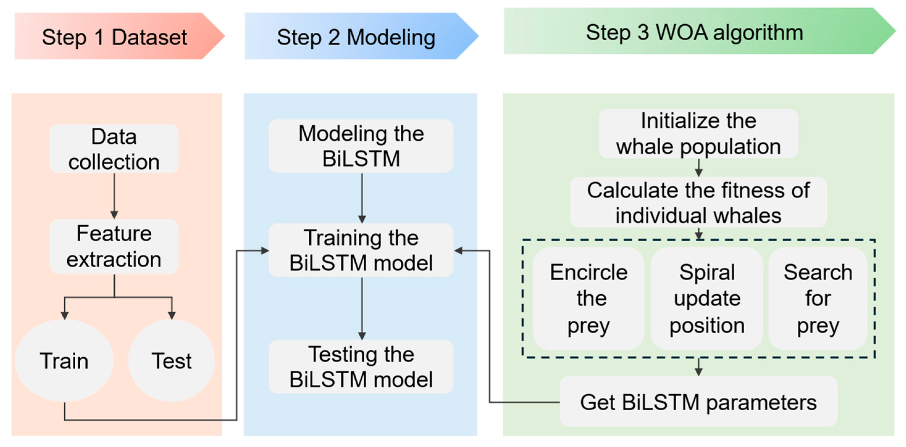
In this study, the WOA is employed to optimize key hyperparameters of the BiLSTM model, including the number of LSTM units, the learning rate of the optimizer, and the batch size. Each whale encodes a candidate configuration of these hyperparameters. The fitness of each whale is evaluated based on the validation error of the corresponding BiLSTM model trained with those settings. Through iterative updates, the WOA converges with the optimal parameter set that yields the best predictive performance. The workflow of the WOA-BiLSTM model is shown in Figure 2.

2.3. Probabilistic Interval Prediction Using Bootstrap

Probabilistic interval prediction is a method used to estimate the possible range of future values at a given confidence level. Unlike traditional deterministic point prediction, probabilistic prediction presents the result as a range defined by an upper and lower bound, as shown in Figure 3a.

Confidence interval (CI) provides an estimate of the error $\epsilon \left(x_t\right)$ between the measured value ${\widehat{y}}_t$ and predicted value $y_t$. It is commonly assumed that data error ${\epsilon }_1\left(x_t\right)$ and model error ${\epsilon }_2\left(x_t\right)$ are independent and both follow a standard normal distribution. Based on these assumptions, the overall prediction error can be expressed as follows:

$${\sigma }_{\epsilon }^2\left(x_t\right)={\sigma }_{{\epsilon }_1}^2\left(x_t\right)+{\sigma }_{{\epsilon }_2}^2\left(x_t\right)$$

(13)

The probability distribution of the unknown value is derived by calculating the total error between the measured and predicted values using probabilistic forecasting methods. Based on this distribution, the prediction interval corresponding to a given confidence level can be determined. For a confidence level of $\alpha$, the prediction interval is expressed as follows [35]:

$$L^{\left(\alpha \right)}\left(x_t\right)={\widehat{y}}_t-z_{1-{\displaystyle \frac{\alpha }{2}}}\sqrt{{\sigma }_{\epsilon }^2\left(x_t\right)}$$

(14)

$$U^{\left(\alpha \right)}\left(x_t\right)={\widehat{y}}_t+z_{1-{\displaystyle \frac{\alpha }{2}}}\sqrt{{\sigma }_{\epsilon }^2\left(x_t\right)}$$

(15)

where $z_{1-\alpha /2}$ denotes the $z_{1-\alpha /2}$ quantile of the standard normal distribution and $L^{\left(\alpha \right)}\left(x_t\right)$ and $U^{\left(\alpha \right)}\left(x_t\right)$ represent the upper and lower bounds of the prediction at time $t$, respectively.

The Bootstrap method is a statistical method for estimating statistics, testing statistical hypotheses, and constructing predictive models by repeatedly sampling from the original dataset. The core concept is based on self-sampling: that is, randomly drawing samples from the original dataset and allowing the same samples to be selected multiple times in different samples to form a resampled dataset of the same size as the original dataset. The characteristic feature of the Bootstrap is that it does not rely on data distribution assumptions and does not require the addition of new samples. Figure 3b shows the basic principle of the Bootstrap.

The principle of the Bootstrap method involves performing sampling with replacement from the original dataset $D$, maintaining the same sample size $N$. Each data point has an equal probability $1/N$ of being selected. By repeating the sampling process $B$ times, multiple Bootstrap datasets are generated and used to train predictive models. The resulting ensemble of model outputs is then used to estimate the target statistical quantity.

Given a random sample $X=[x_1,x_1,\cdots x_n]$ drawn from an unknown distribution, let $P_n$ denote the empirical distribution function of the sample $X$. Suppose the parameter of interest is $\theta$, and $\widehat{y}$ is an estimator of $\theta$. Through Bootstrap resampling, $B$ independent Bootstrap sub-samples of size $N$ are generated, denoted as $X_b^{*}=[x_{1,b}^{*},x_{2,b}^{*},\cdots ,x_{n,b}^{*}]$, where $b=\mathrm{1,2},\cdots B$. The estimator is computed for each Bootstrap sample, yielding $y_1^{*},y_2^{*},\cdots ,y_B^{*}$. For the random variable $\theta$, the mean and standard deviation of the Bootstrap sample are as follows:

$${\overline{y}}^{*}={\displaystyle \frac{1}{B}}{\sum }_{i=1}^B{y}_i^{*}$$

(16)

$${\sigma }_{{\overline{y}}^{*}}^2={\displaystyle \frac{1}{B-1}}{\sum }_{i=1}^B{{(\theta }_i^{*}-{\overline{\theta }}^{*})}^2$$

(17)

where ${\sigma }_{{\overline{y}}^{*}}$ represents the model variance, reflecting the variance due to different parameters of the neural network model. The confidence interval of the model at confidence level $\alpha$ is denoted as follows:

$${CI}_{{\epsilon }_2}={\overline{y}}^{*}\pm z_{1-{\displaystyle \frac{\alpha }{2}}}\sqrt{{\sigma }_{{\overline{y}}^{*}}^2}$$

(18)

The data variance of the resampled dataset was estimated with the following formula:

$${\sigma }_{{\epsilon }_1}^2\cong {\displaystyle \frac{1}{B-1}}{\sum }_{b=1}^B{{(y}_i^{*}-y^{*})}^2-{\sigma }_{{\overline{y}}^{*}}^2$$

(19)

where ${\sigma }_{{\epsilon }_1}^2$ is the noise variance. Since noise cannot be negative, the estimate of noise variance A is expressed as follows:

$$r^2=\mathit{max}\left({\sigma }_{{\epsilon }_1}^2,0\right)$$

(20)

Considering that there will be zero values in the noisy variance set, the noise variance is replaced with the predicted values to reduce the stochastic effect of the noise variance on the results, and a new data set $D_z$ is obtained.

$$D_z=\left\{\left(x_n,r^2\right)\right\}$$

(21)

The noise variance is obtained by constructing a new model from dataset $D_z$. When training the new model, it is trained by the maximum likelihood method to maximize the probability of the occurrence of the noise variance in the observed samples. The objective function is given below:

$$C_N={\displaystyle \frac{1}{2}}{\sum }_{i=1}^N\left[{\displaystyle \frac{r_i^2}{{\sigma }_{\epsilon }^2\left(x_i\right)}}+\mathit{ln}\left({\sigma }_{\epsilon }^2\left(x_i\right)\right)\right]$$

(22)

By combining the estimated data variance and model variance, the upper and lower bounds of the prediction interval can be calculated using Equations (14) and (15), thereby enabling the quantification of prediction uncertainty.

3. Experimental Data and Feature Extraction

3.1. Oxford Dataset

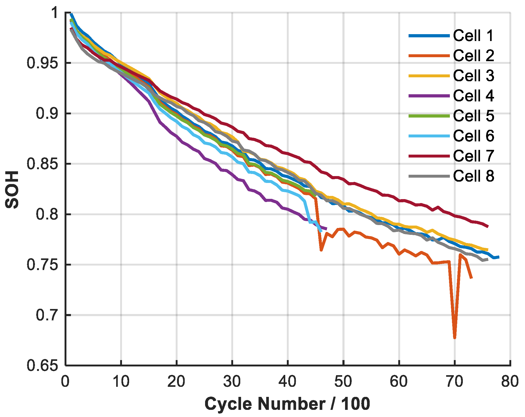
This work utilizes an aging battery dataset collected by the University of Oxford, comprising eight Kokam pouch cells with a nominal capacity of 0.74 Ah, designated as cell 1 to cell 8. The anode of the cells is graphite, and the cathode is a mixture of lithium cobalt oxide (LCO) and lithium nickel cobalt oxide (NCO) [11]. Key technical specifications are summarized in

Table 1. Parameters of Oxford aging test.

Cell Type	Electrode Material	Rated Capacity/Ah	Discharge Cut-Off Voltage/V	Charge Cut-Off Voltage/V	Temperature
Pouch	LCO, NCO	0.74	2.7	4.2	40 °C

. During testing, cells were charged at a constant current rate of 2C, while discharge followed the Artemis Urban Driving Cycle to emulate realistic operating conditions. Capacity assessments were performed at intervals of 100 cycles. All experiments were carried out at a constant ambient temperature of 40 °C, with a data sampling rate of 1 Hz. The capacity aging trends of the eight cells are depicted in Figure 4.

3.2. IC and DV Curves

To investigate the degradation mechanisms during cycling, Incremental Capacity Analysis (ICA) and Differential Voltage Analysis (DVA) were performed on the lithium-ion battery dataset. These analyses are based on differential transformations of voltage and capacity signals, which can reveal subtle electrochemical changes during battery aging. Specifically, ICA involves calculating the derivative of capacity to voltage (dQ/dV), typically during the charging process, while DVA calculates the derivative of voltage to capacity (dV/dQ), usually during the discharge process. Charging curves generally exhibit smoother voltage–capacity profiles, less influenced by relaxation or rate effects, resulting in ICA peaks that more clearly reflect electrode phase transitions and loss of lithium inventory. In contrast, discharge curves tend to be more sensitive to polarization and internal resistance growth, enabling DVA to effectively capture shifts in voltage plateaus and peak positions indicative of impedance-related degradation [40,41]. These curves reflect the phase transitions, reaction kinetics, and internal resistance evolution within the electrode material. To suppress noise and enhance feature clarity, Gaussian smoothing was applied to the raw curves with a standard deviation ($\sigma$) of 10. Four cycles were selected for visualization and analysis, spanning the early, mid, and advanced aging stages, which enabled clear observation of the evolving electrochemical signatures. The smoothed IC and DV curves of cell 1 are shown in Figure 5. This cell was selected because it had a complete and continuous data set throughout the entire cycle test, with no missing or abnormal data points due to experimental interference.

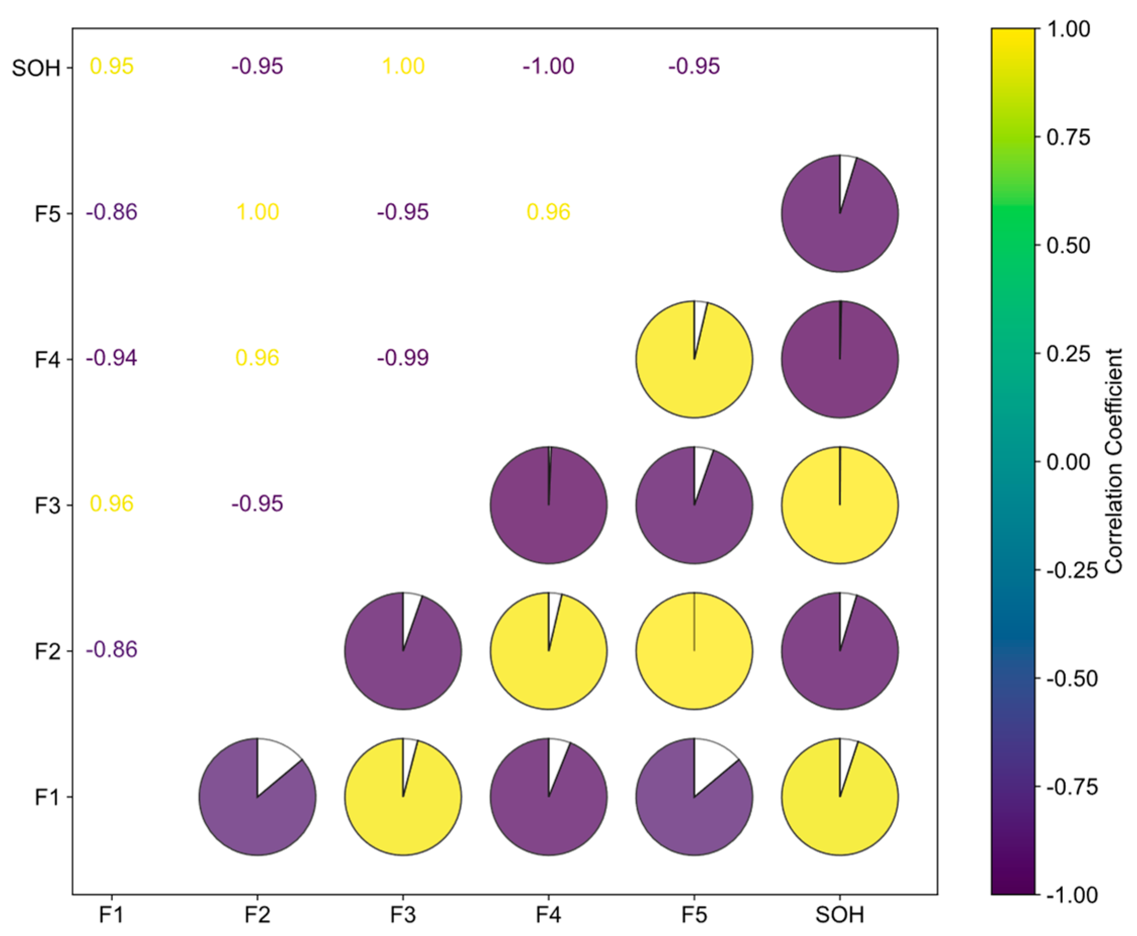
The morphological characteristics of the peaks and valleys in the IC and DV curves, especially the height, position, and size, are considered as key indicators of battery aging. These characteristics change significantly with cycling and can reflect changes in electrochemical reaction kinetics, electrode phase transition, and internal resistance. According to Figure 5, it can be noted that the IC peak, the corresponding voltage, and the area below the peak decrease or increase with cell aging. These features can be used to react to the cell aging trend. Compared with ICA, the valley feature of the DV curve is sensitive to changes in electrode polarization and capacity loss. So, we extracted the valley value and the voltage corresponding to the valley value as the feature inputs, as shown in

Table 2. Summary of extracted features from IC and DV curves.

Feature	Source Curve	Definition
F1	IC	Peak value of IC curve
F2	IC	Voltage corresponding to IC curve peak
F3	IC	Integrated area under the peak region
F4	DV	Valley value of DV curve
F5	DV	Voltage corresponding to DV curve valley

. To assess the correlation of selected features with battery aging, we quantified them using the Pearson correlation coefficient, as shown in Figure 6. It quantifies the strength and direction of a linear relationship, ranging from –1 to +1. Features with higher absolute values are more strongly associated with SOH variations, indicating higher predictive power. The correlations of these features with SOH are all greater than 0.9, showing a strong relationship, and thus can be used as inputs to the SOH prediction deep learning model.

3.3. Evaluation Metrics

For model evaluation, the mean absolute error (MAE), the mean absolute percentage error (MAPE), and the root mean square error (RMSE) are used to measure the performance of SOH prediction model. These metrics are defined as follows:

$$MAE={\displaystyle \frac{1}{n}}{\sum }_{i=1}^n|\widehat{y_i}-y_i|$$

$$RMSE=\sqrt{{\displaystyle \frac{1}{n}}{\sum }_{i=1}^n{(\widehat{y_i}-y_i)}^2}$$

$$MAPE={\displaystyle \frac{100\mathrm{\%}}{n}}{\sum }_{i=1}^n|{\displaystyle \frac{\widehat{y_i}-y_i}{y_i}}|$$

where $n$ denotes the total number of test samples and $y_i$ and $\widehat{y_i}$ represent the true value and predicted value, respectively.

Unlike the RMSE and MAE metrics that characterize point prediction results, the Prediction Interval Coverage Probability (PICP), Prediction Interval Normalized Average Width (PINAW), and Coverage Width-based Criterion (CWC) reflect the accuracy of the interval predictions at confidence level $\alpha$. PICP is used to assess the coverage of the prediction interval over the true value. A larger value of PICP indicates a higher probability that the true value is within the prediction interval. It can be calculated as follows:

$$PICP={\displaystyle \frac{1}{n}}{\sum }_{i=1}^n{c}_i$$

where when $y_i \in [L_i,U_i]$, then $c_i=1$, otherwise $c_i=0$. $L_i$ and $U_i$ denote the lower and upper bounds of the $i$-th prediction interval, respectively.

PINAW represents the normalized average width of prediction intervals relative to the range of actual values. When the prediction width is wide enough, PICP reaches 1 and the prediction results lose their reference. Therefore, PINAW is introduced to evaluate the compactness of prediction intervals.

$$PINAW={\displaystyle \frac{1}{nR}}{\sum }_{i=1}^n(U_i-L_i)$$

where $R$ stands for the difference between the maximum and minimum values of the test set for normalization calculations.

It is difficult to comprehensively evaluate the prediction intervals by focusing only on predicting PICP or PINAW. Therefore, combining the coverage and width of the prediction intervals, CWC is introduced to evaluate the prediction results.

$$CWC=PINAW(1+\gamma e^{-\eta \left(PICP-\mu \right)})$$

where $\gamma$ is depend on PICP, $\gamma =\left\{\begin{array}{c}0,PICP\ge \mu \\ 1,PICP\le \mu \end{array}\right.$.

4. Results and Discussion

4.1. Deterministic Prediction Results

To comprehensively evaluate the effectiveness of the proposed WOA-BiLSTM model in predicting lithium-ion battery SOH, we conducted a comparative analysis against three widely used deep learning models: LSTM, BiLSTM, and BiGRU. All models were trained under consistent hyperparameter settings and provided with identical IC/DV-based input features to ensure a fair comparison.

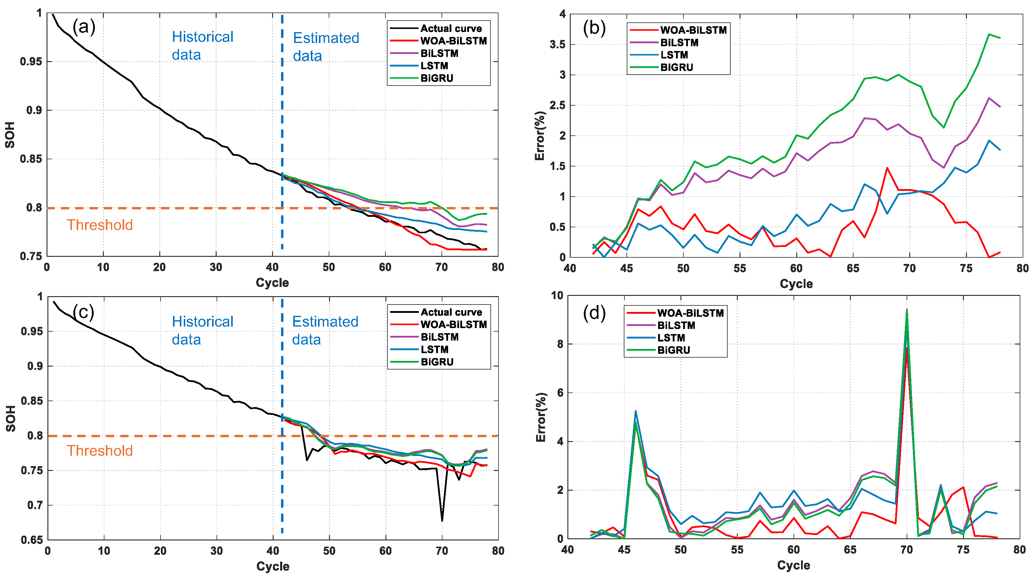
Figure 7 shows the SOH estimation curves and errors of cell 1 and cell 2, respectively. The first 50% is the training set and the rest is employed as the test set. All four models can roughly describe the trend of SOH changes, but the WOA-BiLSTM model achieved the lowest prediction error and the highest correlation with the true SOH values, demonstrating superior accuracy and robustness. Compared to the standard LSTM model, the WOA-BiLSTM benefits from richer temporal context modeling, as the bidirectional structure enables it to extract degradation trends not only from past cycles but also in reverse, enhancing the model’s temporal sensitivity. Compared to BiGRU, while both models share bidirectional architectures, the gating mechanism in LSTM is more expressive for long-term dependencies, which may explain the consistently better performance of BiLSTM-based models in our experiments. Despite the advantages, it is worth noting that the integration of the WOA introduces additional computational cost during training. However, since the optimization is performed offline, it does not impact the inference time, making the approach suitable for deployment in real-time battery management systems.

To investigate the robustness and generalization ability of the proposed WOA-BiLSTM framework, the performance of the model was compared when using three different proportions of training data (30%, 40%, and 50% of the total lifecycle) over multiple prediction starting points. Figure 8 demonstrates the SOH estimation curves with different starting points. The results show that the WOA-BiLSTM model maintains stable performance with RMSE values below 3%, even with limited historical data. Thus, the model effectively captures key degradation patterns without relying excessively on specific parts of the cycle life. This robustness is beneficial for practical applications where historical data may be limited.

The evaluation metric results for SOH estimation of all eight cells are summarized in

Table 3. SOH estimation errors for different models for all eight cells.

Battery No.	Model	RMSE/%	MAE/%	MAPE/%
Cell 1	WOA-BiLSTM	0.62	0.50	0.64
	BiLSTM	1.64	1.52	1.95
	LSTM	0.86	0.71	0.91
	BiGRU	2.15	1.95	2.50
Cell 2	WOA-BiLSTM	1.75	0.94	1.26
	BiLSTM	2.22	1.45	1.95
	LSTM	2.13	1.46	1.95
	BiGRU	2.15	1.35	1.82
Cell 3	WOA-BiLSTM	0.44	0.34	0.43
	BiLSTM	0.78	0.63	0.76
	LSTM	1.03	0.94	1.20
	BiGRU	1.20	0.96	1.23
Cell 4	WOA-BiLSTM	0.48	0.36	0.45
	BiLSTM	1.34	1.46	1.37
	LSTM	1.06	0.98	1.21
	BiGRU	2.71	2.38	2.96
Cell 5	WOA-BiLSTM	0.25	0.20	0.23
	BiLSTM	0.65	0.56	0.67
	LSTM	1.22	1.03	1.17
	BiGRU	1.83	1.46	1.75
Cell 6	WOA-BiLSTM	0.64	0.43	0.52
	BiLSTM	0.79	0.73	0.88
	LSTM	0.71	0.62	0.75
	BiGRU	1.01	0.54	0.76
Cell 7	WOA-BiLSTM	0.41	0.31	0.38
	BiLSTM	0.82	0.75	0.93
	LSTM	1.52	1.33	1.71
	BiGRU	1.58	1.35	1.67
Cell 8	WOA-BiLSTM	0.43	0.36	0.46
	BiLSTM	0.20	0.15	0.19
	LSTM	0.73	0.62	0.79
	BiGRU	1.72	1.51	1.94

. Across all cases, the proposed WOA-BiLSTM model achieves the lowest RMSE, MAE, and MAPE values compared with BiLSTM, LSTM, and GRU, demonstrating consistent advantages in prediction accuracy. For cell 1, the RMSE, MAPE and MAE of the WOA-BiLSTM model are 0.62%, 0.64%, and 0.50%, respectively. For cell 2, despite the slight increase in error, the WOA-BiLSTM still outperforms the other three baseline models with an RMSE of 1.75%, MAE of 0.94%, and MAPE of 1.26%. Similar trends are observed for the remaining cells (cells 3–8), with all RMSE values remaining within an acceptable range, indicating strong generalization capability. These consistent improvements confirm the effectiveness and robustness of the proposed model in handling complex degradation dynamics and enhancing SOH estimation reliability.

4.2. Probabilistic Prediction Results

The point estimation performance of the WOA-BiLSTM model for SOH prediction is validated in Section 4.1. To further assess the reliability and uncertainty quantification capability of the model, this section explores the probabilistic prediction performance by integrating the Bootstrap resampling technique into the WOA-BiLSTM framework, considering two confidence levels of 80% and 90%.

The probabilistic prediction results for cell 1 and cell 2 are shown in Figure 9. It can be found that the 90% confidence interval is relatively narrow and contains relatively few prediction points, while the 80% confidence interval can contain all the actual capacity points. For cell 2, although significant fluctuations appear in the later degradation stage, the 80% confidence interval still includes most of the actual SOH values. This suggests that the model effectively captures the inherent uncertainty, even under aggressive aging conditions. The robustness of the interval prediction under such circumstances highlights the model’s adaptability to variable degradation patterns and its potential for generalization.

The quantitative evaluation of the probabilistic prediction results at 80% and 90% confidence levels is shown in

Table 4. Evaluation results at 80% and 90% confidence levels.

Battery No.	PICP		PINAW		CWC
	90%	80%	90%	80%	90%	80%
Cell 1	0.95	1	0.41	0.47	0.41	0.47
Cell 2	0.86	1	0.31	0.37	0.31	0.37

. The experimental results indicate that the WOA-BiLSTM intervals effectively capture the variability and uncertainty associated with SOH degradation. For both confidence levels, the PICP values are close to their nominal confidence levels, demonstrating that the model reliably estimates intervals that encompass the true SOH values with high probability. Specifically, under the 80% confidence level, the PICP achieves 1, reflecting strong coverage performance. At the 90% level, PICP values remained above 0.86 across different test sets, further validating the reliability of the interval estimation process. In terms of interval width, the PINAW increased with confidence level, as expected. The average width of the 80% intervals was notably wider than that of the 90% intervals, reflecting a trade-off between coverage and sharpness. While wider intervals are associated with higher coverage, excessively large widths reduce the utility of predictions in practical battery management applications.

Interestingly, in the current results, the values of PINAW and CWC were found to be nearly identical or even exactly equal under certain conditions. This behavior can be attributed to the internal formulation of the CWC metric, which is defined in Equations (1) and (2). When the PICP meets or exceeds the nominal confidence level (i.e., $PICP\ge \mu$), the exponential penalty term becomes negligible or zero. In this case, the CWC can be simplified to PINAW. Therefore, the equality between CWC and PINAW indicates that the model achieves sufficient coverage and the prediction intervals are not only narrow but also statistically reliable. This observation also emphasizes the importance of interpreting CWC in conjunction with PICP. A low CWC that equals PINAW is only meaningful when PICP is close to or above the target confidence level. If PICP were below the threshold, CWC would automatically increase due to the exponential penalty. Thus, consistent equality between PINAW and CWC provides indirect evidence of the model’s robustness in meeting interval coverage targets.

5. Conclusions

In this work, we developed a probabilistic data-driven SOH prediction model that integrates electrochemical feature extraction and deep learning models. By combining IC and DV features as model inputs, the proposed framework leverages key aging signatures inherent in charge–discharge processes. The WOA algorithm effectively optimizes the BiLSTM network, enhancing prediction accuracy. Compared with conventional models such as LSTM, BiLSTM, and BiGRU, the WOA-BiLSTM model demonstrated significantly improved performance in terms of both error metrics and generalization capability.

Furthermore, by incorporating the Bootstrap method, the model is extended to provide probabilistic interval predictions. These intervals offer uncertainty estimates, with consistent coverage at both 80% and 90% confidence levels. The results show that PICP reaches 1 at the 80% confidence level and exceeds 0.85 at the 90% confidence level, with PINAW and CWC metrics validating the interval quality. In particular, the model maintains robust performance even in later degradation stages and under high-rate cycling conditions.

Despite these promising results, some limitations remain. While the Bootstrap approach provides a non-parametric estimation of uncertainty, it may not capture epistemic uncertainty arising from limited training data or distribution shifts. Future work will explore more advanced uncertainty quantification methods, such as Bayesian Deep Learning, to further enhance the model’s applicability in complex battery systems. Additionally, the current framework is primarily evaluated on standard laboratory datasets, and its generalizability to large-scale, heterogeneous battery systems remains to be validated.

References

1. Guo, S.; Ma, L. A Comparative Study of Different Deep Learning Algorithms for Lithium-Ion Batteries on State-of-Charge Estimation. Energy 2023, 263, 125872. [Google Scholar] [CrossRef]
2. Vennam, G.; Sahoo, A.; Ahmed, S. A Survey on Lithium-Ion Battery Internal and External Degradation Modeling and State of Health Estimation. J. Energy Storage 2022, 52, 104720. [Google Scholar] [CrossRef]
3. Ng, M.F.; Zhao, J.; Yan, Q.; Conduit, G.J.; Seh, Z.W. Predicting the state of charge and health of batteries using data-driven machine learning. Nat. Mach. Intell. 2020, 2, 161–170. [Google Scholar] [CrossRef]
4. Whittingham, M.S. History, Evolution, and Future Status of Energy Storage. Proc. IEEE 2012, 100, 1518–1534. [Google Scholar] [CrossRef]
5. Feng, X.; Pan, Y.; He, X.; Wang, L.; Ouyang, M. Detecting the Internal Short Circuit in Large-Format Lithium-Ion Battery Using Model-Based Fault-Diagnosis Algorithm. J. Energy Storage 2018, 18, 26–39. [Google Scholar] [CrossRef]
6. Zhao, J.; Tian, L.; Cheng, L. Review on State Estimation and Remaining Useful Life Prediction Methods for Lithium-Ion Battery. Power Gener. Technol. 2023, 44, 1–17. [Google Scholar] [CrossRef]
7. Sun, T.; Xu, B.; Cui, Y.; Feng, X.; Han, X.; Zheng, Y. A Sequential Capacity Estimation for the Lithium-Ion Batteries Combining Incremental Capacity Curve and Discrete Arrhenius Fading Model. J. Power Sources 2021, 484, 229248. [Google Scholar] [CrossRef]
8. Han, X.; Wang, Z.; Wei, Z. A Novel Approach for Health Management Online-Monitoring of Lithium-Ion Batteries Based on Model-Data Fusion. Appl. Energy 2021, 302, 117511. [Google Scholar] [CrossRef]
9. Xia, F.; Wang, K.; Chen, J. State of Health and Remaining Useful Life Prediction of Lithium-Ion Batteries Based on a Disturbance-Free Incremental Capacity and Differential Voltage Analysis Method. J. Energy Storage 2023, 64, 107161. [Google Scholar] [CrossRef]
10. Lin, M.; Wu, D.; Meng, J.; Wu, J.; Wu, H. A Multi-Feature-Based Multi-Model Fusion Method for State of Health Estimation of Lithium-Ion Batteries. J. Power Sources 2022, 518, 230774. [Google Scholar] [CrossRef]
11. Zhou, D.; Wang, B. Battery Health Prognosis Using Improved Temporal Convolutional Network Modeling. J. Energy Storage 2022, 51, 104480. [Google Scholar] [CrossRef]
12. Torai, S.; Nakagomi, M.; Yoshitake, S.; Yamaguchi, S.; Oyama, N. State-of-Health Estimation of LiFePO4/Graphite Batteries Based on a Model Using Differential Capacity. J. Power Sources 2016, 306, 62–69. [Google Scholar] [CrossRef]
13. Messing, M.; Shoa, T.; Habibi, S. Estimating Battery State of Health Using Electrochemical Impedance Spectroscopy and the Relaxation Effect. J. Energy Storage 2021, 43, 103210. [Google Scholar] [CrossRef]
14. Huang, Z.; Best, M.; Knowles, J.; Fly, A. Adaptive Piecewise Equivalent Circuit Model With SOC/SOH Estimation Based on Extended Kalman Filter. IEEE Trans. Energy Convers. 2023, 38, 959–970. [Google Scholar] [CrossRef]
15. Vennam, G.; Sahoo, A. A Dynamic SOH-Coupled Lithium-Ion Cell Model for State and Parameter Estimation. IEEE Trans. Energy Convers. 2023, 38, 1186–1196. [Google Scholar] [CrossRef]
16. Shrivastava, P.; Soon, T.K.; Idris, M.Y.I.B.; Mekhilef, S. Overview of Model-Based Online State-of-Charge Estimation Using Kalman Filter Family for Lithium-Ion Batteries. Renew. Sustain. Energy Rev. 2019, 113, 109233. [Google Scholar] [CrossRef]
17. Chen, L.; Yu, W.; Cheng, G.; Wang, J. State-of-Charge Estimation of Lithium-Ion Batteries Based on Fractional-Order Modeling and Adaptive Square-Root Cubature Kalman Filter. Energy 2023, 271, 127007. [Google Scholar] [CrossRef]
18. Chen, C.; Xiong, R.; Yang, R.; Li, H. A Novel Data-Driven Method for Mining Battery Open-Circuit Voltage Characterization. Green Energy Intell. Transp. 2022, 1, 100001. [Google Scholar] [CrossRef]
19. Meng, H.; Geng, M.; Han, T. Long Short-Term Memory Network with Bayesian Optimization for Health Prognostics of Lithium-Ion Batteries Based on Partial Incremental Capacity Analysis. Reliab. Eng. Syst. Saf. 2023, 236, 109288. [Google Scholar] [CrossRef]
20. He, J.; Bian, X.; Liu, L.; Wei, Z.; Yan, F. Comparative Study of Curve Determination Methods for Incremental Capacity Analysis and State of Health Estimation of Lithium-Ion Battery. J. Energy Storage 2020, 29, 101400. [Google Scholar] [CrossRef]
21. Zhou, Q.; Anderson, D.; Sun, J. State of Health Estimation for Battery Modules with Parallel-Connected Cells under Cell-to-Cell Variations. eTransportation 2024, 22, 100346. [Google Scholar] [CrossRef]
22. Wang, L.; Pan, C.; Liu, L.; Cheng, Y.; Zhao, X. On-Board State of Health Estimation of LiFePO4 Battery Pack through Differential Voltage Analysis. Appl. Energy 2016, 168, 465–472. [Google Scholar] [CrossRef]
23. Li, Y.; Abdel-Monem, M.; Gopalakrishnan, R.; Berecibar, M.; Nanini-Maury, E.; Omar, N.; van den Bossche, P.; Van Mierlo, J. A Quick On-Line State of Health Estimation Method for Li-Ion Battery with Incremental Capacity Curves Processed by Gaussian Filter. J. Power Sources 2018, 373, 40–53. [Google Scholar] [CrossRef]
24. Klass, V.; Behm, M.; Lindbergh, G. A Support Vector Machine-Based State-of-Health Estimation Method for Lithium-Ion Batteries under Electric Vehicle Operation. J. Power Sources 2014, 270, 262–272. [Google Scholar] [CrossRef]
25. Lin, C.; Xu, J.; Jiang, D.; Hou, J.; Liang, Y.; Zou, Z.; Mei, X. Multi-Model Ensemble Learning for Battery State-of-Health Estimation: Recent Advances and Perspectives. J. Energy Chem. 2025, 100, 739–759. [Google Scholar] [CrossRef]
26. Thelen, A.; Huan, X.; Paulson, N.; Onori, S.; Hu, Z.; Hu, C. Probabilistic Machine Learning for Battery Health Diagnostics and Prognostics—Review and Perspectives. npj Mater. Sustain. 2024, 2, 14. [Google Scholar] [CrossRef]
27. Bamati, S.; Chaoui, H. Lithium-Ion Batteries Long Horizon Health Prognostic Using Machine Learning. IEEE Trans. Energy Convers. 2022, 37, 1176–1186. [Google Scholar] [CrossRef]
28. Tang, A.; Huang, Y.; Xu, Y.; Hu, Y.; Yan, F.; Tan, Y.; Jin, X.; Yu, Q. Data-Physics-Driven Estimation of Battery State of Charge and Capacity. Energy 2024, 294, 130776. [Google Scholar] [CrossRef]
29. Jia, C.; Tian, Y.; Shi, Y.; Jia, J.; Wen, J.; Zeng, J. State of Health Prediction of Lithium-Ion Batteries Based on Bidirectional Gated Recurrent Unit and Transformer. Energy 2023, 285, 129401. [Google Scholar] [CrossRef]
30. Chen, Y.; Huang, X.; He, Y.; Zhang, S.; Cai, Y. Edge–Cloud Collaborative Estimation Lithium-Ion Battery SOH Based on MEWOA-VMD and Transformer. J. Energy Storage 2024, 99, 113388. [Google Scholar] [CrossRef]
31. Saha, B.; Goebel, K.; Poll, S.; Christophersen, J. Prognostics Methods for Battery Health Monitoring Using a Bayesian Framework. IEEE Trans. Instrum. Meas. 2009, 58, 291–296. [Google Scholar] [CrossRef]
32. Liu, K.; Shang, Y.; Ouyang, Q.; Widanage, W.D. A Data-Driven Approach with Uncertainty Quantification for Predicting Future Capacities and Remaining Useful Life of Lithium-Ion Battery. IEEE Trans. Ind. Electron. 2021, 68, 3170–3180. [Google Scholar] [CrossRef]
33. Lin, Y.H.; Li, G.H. A Bayesian Deep Learning Framework for RUL Prediction Incorporating Uncertainty Quantification and Calibration. IEEE Trans. Ind. Inform. 2022, 18, 7274–7284. [Google Scholar] [CrossRef]
34. Wang, Y.; Zhu, J.; Cao, L.; Liu, J.; You, P.; Gopaluni, B.; Cao, Y. A Generalizable Method for Capacity Estimation and RUL Prediction in Lithium-Ion Batteries. Ind. Eng. Chem. Res. 2024, 63, 345–357. [Google Scholar] [CrossRef]
35. Gou, B.; Xu, Y.; Feng, X. State-of-Health Estimation and Remaining-Useful-Life Prediction for Lithium-Ion Battery Using a Hybrid Data-Driven Method. IEEE Trans. Veh. Technol. 2020, 69, 10854–10867. [Google Scholar] [CrossRef]
36. Lin, C.P.; Cabrera, J.; Yang, F.; Ling, M.H.; Tsui, K.L.; Bae, S.J. Battery State of Health Modeling and Remaining Useful Life Prediction through Time Series Model. Appl. Energy 2020, 275, 115338. [Google Scholar] [CrossRef]
37. Li, S.; Jiang, Z.; Zhu, Z.; Jiang, W.; Ma, Y.; Sang, X.; Yang, S. A Framework of Joint SOC and SOH Estimation for Lithium-Ion Batteries: Using BiLSTM as a Battery Model. J. Power Sources 2025, 635, 236342. [Google Scholar] [CrossRef]
38. Li, J.; Ye, M.; Wang, Y.; Wang, Q.; Wei, M. A Hybrid Framework for Predicting the Remaining Useful Life of Battery Using Gaussian Process Regression. J. Energy Storage 2023, 66, 107513. [Google Scholar] [CrossRef]
39. Nasiri, J.; Khiyabani, F.M. A Whale Optimization Algorithm (WOA) Approach for Clustering. Cogent Math. Stat. 2018, 5, 1483565. [Google Scholar] [CrossRef]
40. Schmitt, C.; Kopljar, D.; Friedrich, K.A. Detailed Investigation of Degradation Modes and Mechanisms of a Cylindrical High-Energy Li-Ion Cell Cycled at Different Temperatures. J. Energy Storage 2025, 120, 116486. [Google Scholar] [CrossRef]
41. Zhang, S.; Guo, X.; Dou, X.; Zhang, X. A Rapid Online Calculation Method for State of Health of Lithium-Ion Battery Based on Coulomb Counting Method and Differential Voltage Analysis. J. Power Sources 2020, 479, 228740. [Google Scholar] [CrossRef]
Figure 1. The structure of a single LSTM network and a BiLSTM network. (a) The traditional LSTM structure. (b) The structure of BiLSTM.
Energies 18 05450 g001
Figure 2. The workflow of the WOA-BiLSTM model.
Energies 18 05450 g002
Figure 3. Probabilistic interval prediction using Bootstrap. (a) Schematic of probabilistic prediction. (b) Principle of the Bootstrap.
Energies 18 05450 g003
Figure 4. Battery SOH for the Oxford laboratory dataset.
Energies 18 05450 g004
Figure 5. IC and DV curves of cell 1. (a) Smoothed IC curves at different cycles, (b) smoothed DV curves at different cycles.
Energies 18 05450 g005
Figure 6. The Pearson correlation coefficient between features and SOH.
Energies 18 05450 g006
Figure 7. SOH estimation curves and errors for different cells. (a,b) Cell 1. (c,d) Cell 2.
Energies 18 05450 g007
Figure 8. SOH estimation curves with different starting points. (a) Cell 1. (b) Cell 2.
Energies 18 05450 g008
Figure 9. Probabilistic prediction results for cell 1 and cell 2. (a) Cell 1. (b) Cell 2.
Energies 18 05450 g009