1. Introduction
Power systems represent critical infrastructure in modern society, where their security and stability directly impact the national economy and people’s livelihoods. With the increasing integration of renewable energy, the expanding scale of power grids, and the growing complexity of operational modes, power systems are confronted with heightened uncertainties and potential risks. In this context, performing accurate reliability assessments and further identifying weak links in the system are of crucial theoretical and practical significance for preventing large-scale blackouts, strengthening grid resilience, and improving the quality of power supply.
Early research on the identification of weak links in power systems primarily focused on indirect approaches grounded in traditional deterministic security analysis [
1], used physical models of the power system and assessed component vulnerability by computing a set of security indices. One common strategy involves simulating the outage of single or multiple components and evaluating whether such events lead to overloads or voltage violations in other parts of the system, thereby identifying critical equipment [
2]. Sensitivity-based methods are also employed to compute the differential sensitivities of power flow or voltage with respect to changes in generator outputs or loads [
3]. Additionally, short-circuit current analysis is applied to evaluate the short-circuit level at each bus and to detect substations where circuit breakers may have inadequate interrupting capability [
4]. Although these approaches offer clear physical interpretability and relatively low computational complexity, they are generally ill-suited for comprehensive N−k contingency screening and for accurately allocating fault responsibility [
5].
To address the limitations of conventional methods, some researchers have proposed structural analysis approaches based on complex network theory [
6]. These techniques model the power system as a topological graph and employ graph-theoretic metrics to assess the importance of nodes or edges, thereby identifying structural vulnerabilities from a purely topological standpoint [
7]. Commonly used metrics include degree centrality, betweenness centrality, and closeness centrality [
8,
9,
10]. These methods are computationally efficient and well-suited for rapid screening of large-scale power grids. Nevertheless, they often overlook the physical properties and operational constraints inherent in power systems, which may lead to evaluations that diverge from actual electrical behavior [
11]. Furthermore, such approaches are unable to quantify the specific contribution of individual components to overall system reliability indices.
With a deeper understanding of outage mechanisms, some researchers have turned to simulation-based risk assessment and cascading-failure simulation methods. These approaches involve simulating numerous contingency scenarios and their subsequent evolution to statistically evaluate the risk levels associated with individual components [
12]. Reference [
13] employs Monte Carlo sampling of contingencies combined with power-flow simulations to estimate the probability that the outage of a specific component may lead to system instability. Studies such as references [
14,
15] develop various cascading-failure models to simulate the entire process from an initial fault to a full blackout, thereby identifying critical components that may trigger cascading events. While these methods are effective in capturing dynamic behaviors and cascading effects, they tend to be computationally demanding and heavily reliant on the accuracy of the underlying models. Building on the principles of power-flow tracing and its application to transmission loss allocation, reference [
16] proposes a method to apportion system-level reliability indices to individual components. This enables the quantification of each component’s contribution to system reliability and supports the identification of weak links. However, this approach only allocates contributions proportionally and does not fully incorporate distinctions among component types, electrical characteristics, or reliability parameters, which limits its practical applicability. In recent years, with the development of explainable artificial intelligence technology, some studies have begun to introduce the SHAP algorithm into power system analysis. Reference [
17] used the SHAP Algorithm to identify the key influencing factors of transient stability by developing a TSA model based on the unbalanced-XGBoost algorithm. Reference [
18] used SHAP to predict the cascading failure risk of systems with high proportions of renewable energy and to identify the key lines affecting the system’s cascading failure risk.
In recent years, advances in artificial intelligence have facilitated the application of machine learning techniques to weak-link identification in power systems. Reference [
19] utilizes support vector machines, taking system operating states as input features and the consequences of component failures as labels, to train a regression model for predicting potential weak links. Data-driven methods exhibit strong nonlinear fitting capabilities and are well-suited for addressing high-dimensional problems under uncertainty. Nevertheless, machine learning models are often treated as black boxes, making it challenging to provide reasonable interpretation or physical insight into their predictions [
20].
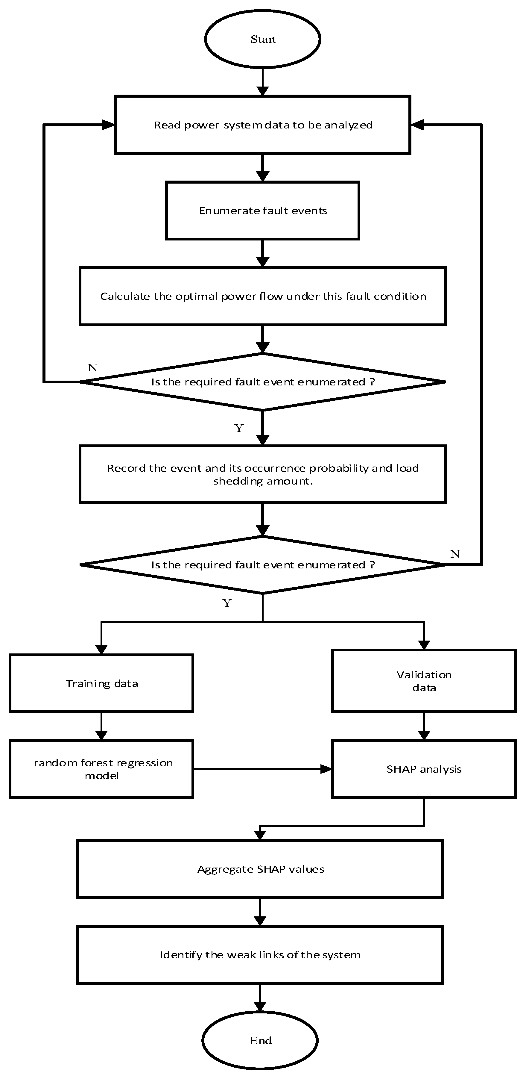
This study integrates random forest regression with SHAP analysis to propose a data-driven framework for reliability attribution and weak-link identification in power systems. Contingency combinations up to third order (N–3) are enumerated, and the corresponding load curtailment, along with the occurrence probability of each contingency, is computed to construct a set of credible contingency scenarios that lead to load loss. A random forest model is trained to learn the nonlinear mapping from contingency events to the resulting load curtailment. SHAP values are then employed to interpret the trained model by quantifying the local contribution of each component to the predicted outcome for a given contingency. Finally, by aggregating the SHAP values of each component across all contingency events, a quantitative measure of its global responsibility for system reliability is derived, thereby providing actionable decision support for identifying critical weak links in the power system.
2. Method for Allocating Reliability Responsibility in Power System
2.1. System State Assessment
This paper conducts a detailed analysis of the generated system operation status one by one to determine whether it can ensure the reliable supply of all electricity loads under the premise of meeting the power flow constraints. The above assessment is often accomplished by solving the following optimal load shedding model; the objective function is to minimize the total load shedding of the entire system, and its calculation is given in (1)
represents the total load shedding quantity of the system; is the set of load nodes; is the load shedding quantity of node . The relevant constraints are as follows:
- (1)
Power balance constraints.
In Formula (2): represents the vector of output variables for generator set; is the vector of load shedding variables; is the vector of active load parameters; is the nodal admittance matrix used for DC power flow calculation; and is the vector of node voltage phase angle variables.
- (2)
Active power output constraint of unit
In Formula (3), represents the collective of generator set; the variables represent the power output of generator set. If the unit is in a fault condition, the values of and are both zero.
- (3)
Line transmission capacity constraints.
When line
is in good condition and operating normally, it must satisfy Equation (4). In the equation,
represents the active power flow through branch
, and
is the transmission capacity limit of this branch; the variables
and
represent the voltage phase at nodes
and
, respectively.
- (4)
Load shedding constraints
In Formula (5), is the active load of node . For a particular operating state , the above model can be constructed and solved to obtain the system-wide load-shedding quantity . If is equal to 0, the system can be reliably supplied in state ; otherwise, the supply is unreliable.
2.2. Power System Reliability Assessment and Dataset Construction
The raw dataset was constructed within an enumeration-based probabilistic reliability assessment framework. This paper enumerates fault combinations of third order and below, calculates the occurrence probability of each fault state and the minimum necessary load shedding under each state, and ultimately obtains the expected value of system load demand reduction through probability weighting. The component outage model adopted in this paper considers two states: normal operation and forced outage, while derated operation and planned outages are not considered.
The fault data includes the combined fault of the generator set and the transmission line. System states were selected via the state enumeration method, and the occurrence probability of an arbitrary system state s is given by Equation (6).
LOLP is the probability that, over a specified period, load is curtailed due to a shortage of generation capacity or network constraints, denoted as
; its calculation is given in (7). EDNS is the expected amount of unmet demand resulting from load curtailment, denoted as
, and its calculation is given in (8).
In the above formulas, denotes the set of system outage states, and denotes the amount of load curtailment in state .
In the consequence analysis, this study utilizes OPF to evaluate system operating conditions under each contingency scenario. We record both LOLP and EDNS when load curtailment occurs, and construct a structured dataset for subsequent reliability assessment. The feature matrix of this dataset consists of system-state vectors corresponding to all enumerated contingency scenarios, with each vector representing a specific contingency event. The target variable is defined as the amount of load curtailment associated with each contingency state.
2.3. Random Forest Regression Model
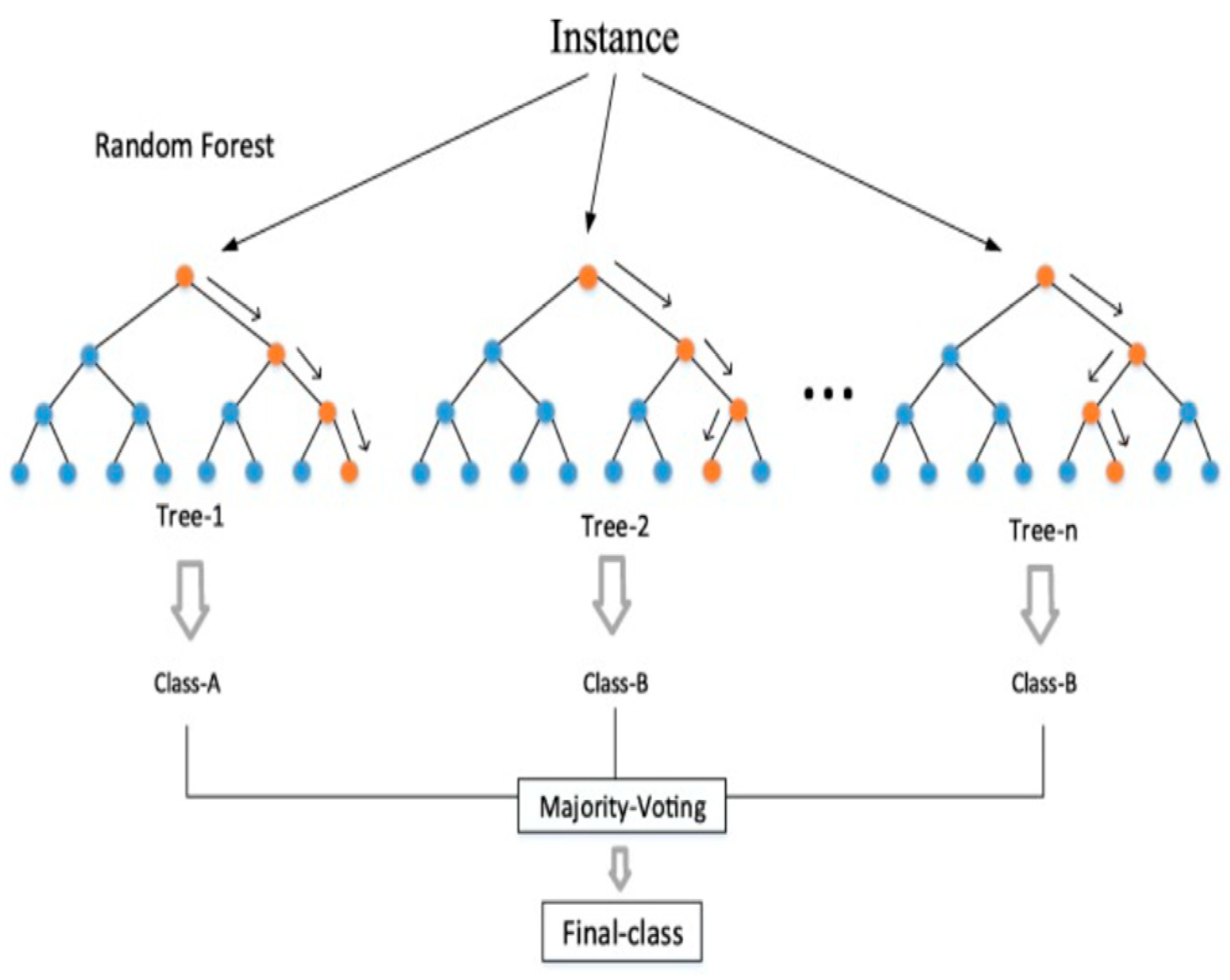
This study utilizes a random forest regression algorithm to establish a nonlinear mapping between system fault states and the corresponding amount of load shedding. As an ensemble learning technique, random forests integrate multiple decision trees to enhance predictive performance and stability. They are capable of effectively capturing interactions among high-dimensional features, while demonstrating robustness to outliers and reduced susceptibility to overfitting. These characteristics render random forests particularly suitable for analyzing reliability datasets that contain numerous Boolean variables, such as the switching states of critical transmission lines.
Bootstrap aggregation (Bagging) and random feature selection constitute two fundamental components of the random forest model. Bagging serves as an ensemble meta-algorithm aimed at improving both the stability and predictive accuracy of machine learning models. The theoretical foundation of Bagging lies in variance reduction, which enhances generalization performance by aggregating predictions from multiple base learners that are homogeneous yet approximately independent. Central to this approach is the bootstrap resampling technique, which entails drawing samples with replacement from the original training dataset to create multiple new training subsets. These subsets are of identical size to the original set but vary in composition due to the random sampling process. Each subset is used to train an individual base learner; the inherent randomness ensures that while some observations are shared across subsets, each also contains unique instances, thereby promoting diversity among the learners.
After training the base learners, Bagging generates the final ensemble prediction through a specific aggregation strategy. In regression tasks, this involves taking the arithmetic mean of the continuous-valued outputs from all base learners. For classification, it employs a majority voting scheme, where the class receiving the highest number of votes is selected as the final prediction. This aggregation process effectively mitigates the influence of noise and idiosyncratic variations present in individual training sets, thereby enhancing the robustness of the ensemble model. Theoretically, by constructing and combining multiple diverse base models, Bagging achieves a significant reduction in overall variance without substantially increasing bias. During training, the algorithm generates multiple bootstrap samples from the original dataset, each of which is used to train an independent decision tree. In constructing each tree, the algorithm incorporates random feature selection; At each node, it randomly draws a subset of features and searches for the optimal split only within this subset. This injected randomness decorrelates the trees and helps prevent overfitting.
As shown in
Figure 1, the induction of a decision tree is a recursive and greedy partitioning process of the feature space. This procedure iteratively partitions the training data into increasingly pure subsets, ultimately forming a tree structure. In the random forest framework, stochastic perturbations are introduced during the construction of each tree: at every node, rather than evaluating all features, the algorithm first samples a random subset of features and selects the optimal split solely from within this subset. This incorporation of stochasticity is essential for promoting diversity across the trees, preventing them from becoming highly correlated, and thereby establishing a foundation for effective ensemble aggregation. Tree growth initiates at the root node, which encompasses the entire bootstrap sample. For each node considered for splitting, the algorithm evaluates all features in the randomly sampled subset along with their candidate thresholds, assessing each potential split using a predefined impurity criterion to measure its quality. The goal is to select the split that achieves the greatest reduction in impurity in the resulting child nodes, thereby maximizing class homogeneity or value similarity within the subsets. This locally optimal, greedy strategy is applied recursively, expanding the tree in a top-down manner.
To fully leverage their role as base (weak) learners and remain consistent with the Bagging framework, decision trees in a random forest are generally grown to maximum depth until predefined stopping criteria are satisfied, without undergoing post-pruning. This unpruned growth strategy allows each tree to closely adapt to the specific characteristics—including noise—of its bootstrap sample, resulting in high variance and low bias. Importantly, these overfitted yet structurally diverse trees are later combined through aggregation, where their high variances counteract each other, leading to strong overall generalization performance for the forest. Therefore, the induction of each decision tree serves not only to capture the underlying structure of the data, but also to intentionally introduce diversity that supports the broader objective of the ensemble.
Regression analysis constitutes a fundamental branch of supervised learning, with the primary objective of predicting a continuous dependent variable based on one or more independent variables. Unlike classification, which produces discrete class labels, regression models learn a mapping function from the input feature space to a continuous real-valued scalar. This output typically represents a physical quantity, an economic indicator, or a measurable outcome—such as house prices, temperature readings, sales figures, or chemical reaction yields. The performance of a regression model is evaluated by measuring the discrepancy between its predictions and the actual values. Commonly used loss functions and evaluation metrics include mean squared error (MSE), root mean squared error (RMSE), and mean absolute error (MAE). These metrics quantify both the magnitude and distribution of prediction errors, thereby offering clear guidance for refining and optimizing the model. For regression tasks, a random forest’s prediction is the average of the predictions from all decision trees. The final prediction of the random forest can be expressed by Equation (9).
In Equation (9), denotes the number of decision trees in the random forest, and denotes the prediction of the tree for input sample b.
2.4. Feature Attribution Analysis Based on SHAP Value
To quantify the contribution of each input feature to the prediction, this study employs SHAP values for feature attribution analysis. As an explainable AI method rooted in cooperative game theory, SHAP quantifies the marginal contribution of each feature to the model’s output, thereby establishing a unified and theoretically grounded framework for model interpretability.
SHAP values are built upon the Shapley value, a concept introduced by Lloyd Shapley in 1953 within the framework of cooperative game theory to address the problem of fair payoff distribution. In the context of machine learning, the prediction task is analogized to a cooperative game where each feature value acts as a player, and the model’s prediction corresponds to the overall payoff. The Shapley value for each feature is computed as specified in Equation (10):
Formula (10) sums over all coalitions that include player ; that is, it enumerates every such coalition and aggregates player i’s contribution to them. indicates the total number of permutations of n players, represents the number of permutations in which the first members of the coalition join first, followed by player i, and then multiplied by the number of permutations for the remaining members to join. After player i joins the coalition, the value they obtain is , which can also be described as the value contributed by player i to the coalition S.
This study employs the TreeSHAP algorithm to calculate SHAP values. TreeSHAP is specifically designed and optimized for tree-based models; it leverages the inherent recursive structure of decision trees to reduce computational complexity from exponential to polynomial time, thereby enabling efficient and exact estimation of each feature’s contribution to individual predictions. For the trained random forest regression model, we compute the SHAP values for every feature across all samples within the test set, resulting in a SHAP value matrix.
SHAP values satisfy two fundamental properties: additivity and consistency. The additivity property ensures that the sum of SHAP values across all features for a given sample equals the difference between the model’s prediction and a baseline value. Consistency guarantees that if a change in the model increases the marginal contribution of a feature, its SHAP value will not decrease—thereby ensuring robust and reliable interpretability. In this application, a positive SHAP value indicates that the outage of a transmission line contributes positively to the amount of load shedding, thereby increasing system unreliability. Conversely, a negative SHAP value implies that the outage reduces load shedding, which typically occurs under specific network configurations where topology changes improve the local balance between supply and demand. By analyzing SHAP values across all samples, we can precisely quantify the influence of each transmission line on system reliability under various fault scenarios, thereby establishing a robust basis for the subsequent allocation of reliability responsibilities.
2.5. Global Reliability Responsibility Allocation
This study adopts a global reliability responsibility allocation method. After obtaining the SHAP values of all lines across all fault scenarios, we quantify at the system level the extent to which each component influences overall reliability, thereby identifying weak links in the system. For each line i, we compute the mean absolute SHAP value as its global reliability responsibility metric, given by (11):
In Equation (11), denotes the total number of fault scenarios, and denotes the SHAP value in fault scenario .
Based on the calculated GRR values, all transmission lines are ranked in descending order; those with the highest rankings are identified as weak links in terms of system reliability. This explainable ML-based methodology offers a novel methodological framework for power system reliability analysis, addressing the shortcomings of conventional approaches in managing higher-order contingencies and capturing intricate system dynamics.
3. Example Analysis
3.1. Test System and Experimental Setup
This study utilizes the IEEE 57-bus test system as a case study to validate the efficacy of the proposed reliability responsibility allocation framework. As illustrated in the single-line diagram in
Figure 2 and
Figure 3, the system consists of 57 buses, 7 generators, 80 transmission lines, and a total load of 1250.8 MW. The computational time of the method proposed in this paper is mainly consumed in the OPF solution for the dataset construction process. The OPF solution takes up more than 90% of the total computational time, while the training of the random forest model and the calculation of SHAP values together account for less than 10%. The OPF solutions for the fault scenarios are independent of each other, and the parallel computing framework can be utilized to distribute the OPF tasks to multiple CPU cores for simultaneous execution. This parallel computing approach can reduce the computational time of the proposed method when dealing with larger-scale actual power grids.
3.2. Random Forest Regression Model Performance
To ensure that the SHAP-based allocation of reliability responsibility is grounded in reliable predictions, this section evaluates the predictive performance of the random forest regression model. Because the model’s predictive accuracy directly determines the credibility of subsequent feature attribution analyses, multiple metrics are employed to validate performance from different perspectives. The metrics are computed as given in Equations (12)–(14).
where
is the observed target,
is the predicted target,
is the mean target of the sample plots, and n is the number of samples.
As shown in
Table 1, the model achieves a high coefficient of determination, indicating that it successfully captures the complex nonlinear relationship between system states and the amount of load shedding. The test-set R
2 is likewise high; the consistency between training- and test-set performance demonstrates good generalization with no apparent overfitting, and the test-set errors remain within a reasonable range.
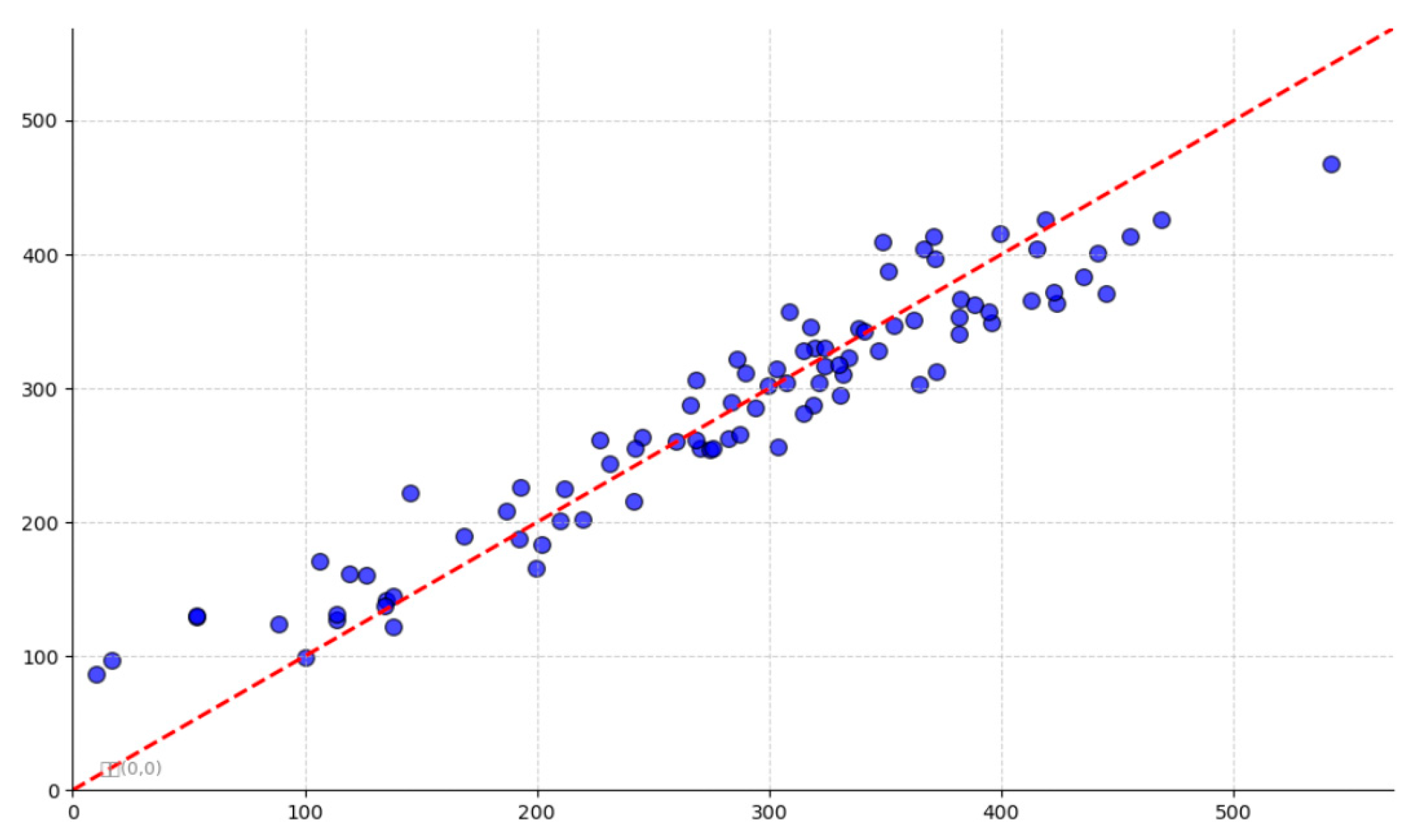
As shown in
Figure 4, the random forest regression model exhibits a good fit on the test set and is able to accurately predict the amount of system cut load under various fault states, which provides a basis for subsequent feature attribution analysis based on SHAP values.
3.3. SHAP Attribution Analysis Results
In this section, the trained random forest model is employed to quantify the nonlinear relationship between component failures and overall system risk. We utilize SHAP for feature attribution analysis and compare the difference between probability-weighted GRR rankings and unweighted average rankings, which ensures that the resulting attributions are both reliable and theoretically sound. SHAP values decompose the model’s predicted load shedding into contributions attributable to each input feature, thereby measuring the marginal influence of individual out-of-service lines on system risk under given conditions.
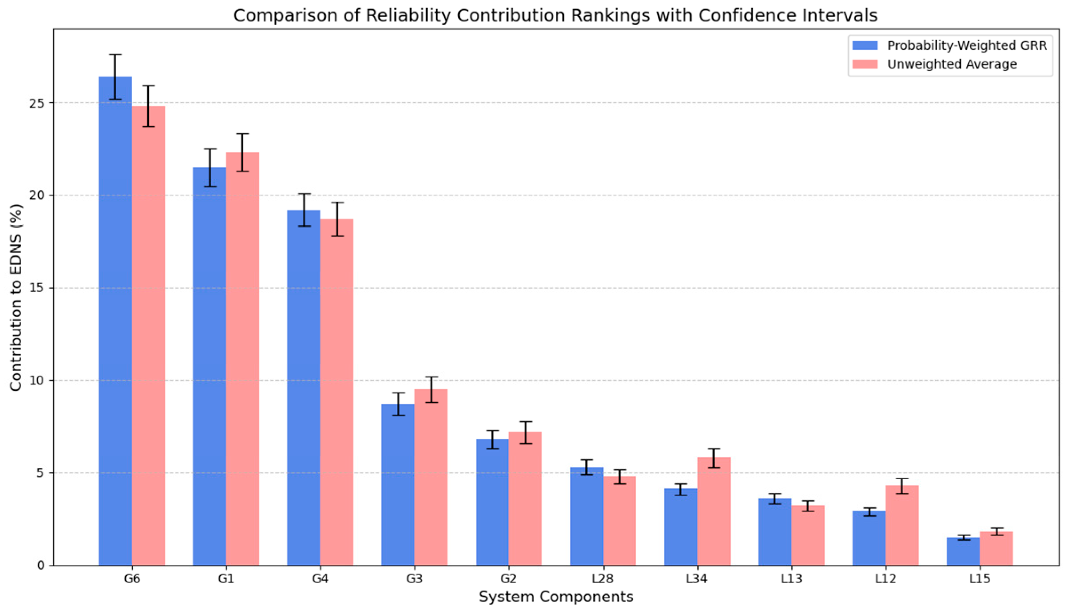
As shown in
Figure 5, the probability-weighted GRR values are generally higher than the unweighted average, indicating that traditional unweighted methods may underestimate the actual reliability impact of critical components. Both methods yield consistent rankings for most components: G6, G1, and G4 consistently rank among the top three, suggesting that these generator components represent the most critical weak points in the system, and their identification remains unaffected by the weighting approach. Among the moderately impactful components, transmission line L34 shows a significant rise in the probability-weighted ranking, indicating that it contributes more substantially to system risk when fault probability is considered. These differences demonstrate that the probability-weighted method places greater emphasis on the actual risk contributions of components with high failure probabilities, whereas the unweighted method tends to average out the effects across different fault scenarios. The probability-weighted GRR approach maintains consistency with traditional methods while more effectively identifying components with both high probability and high impact, thereby providing more accurate decision-making support for system reliability optimization.
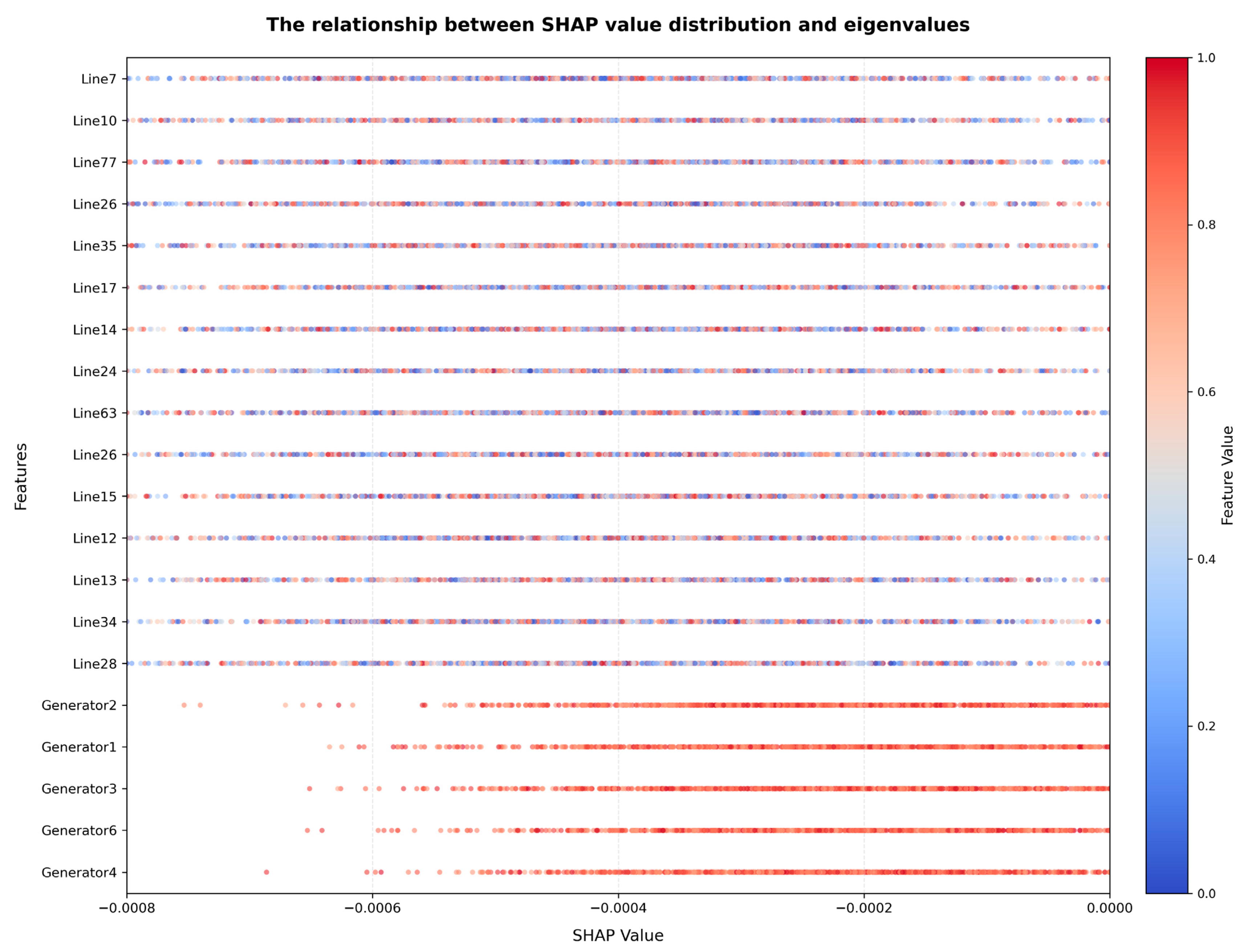
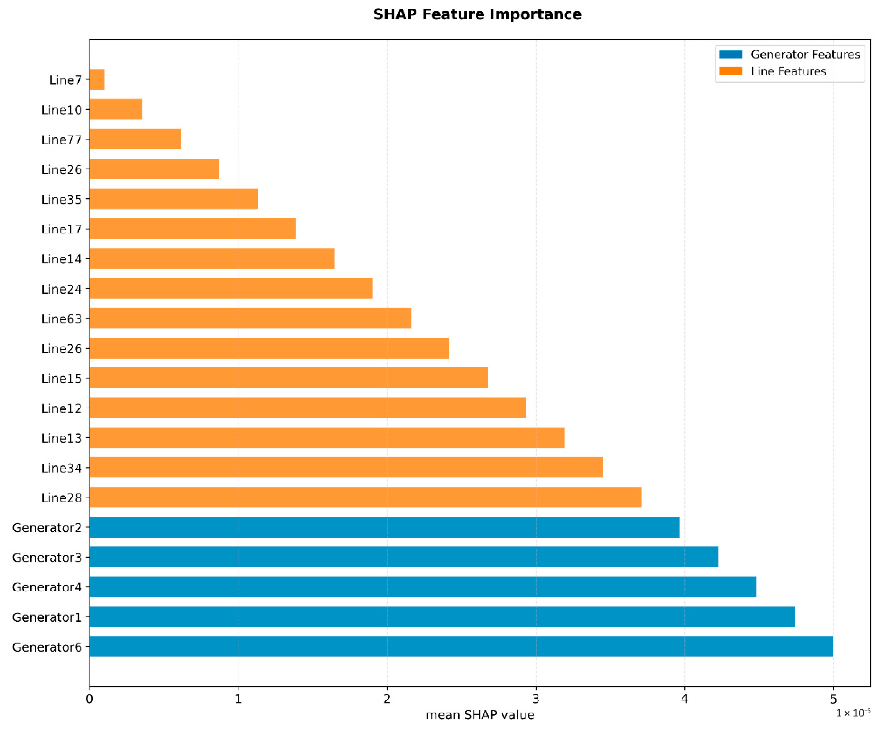
This paper evaluates the influence of random forest model initialization on ranking stability by setting different random seeds. It is found that the GRR ranking of G6, G1 and G4 has high stability, and its 95% confidence interval range is narrow, which proves that the GRR ranking is not sensitive to the randomness of model initialization. As demonstrated by the SHAP-based feature importance rankings in
Figure 6 and
Figure 7, SHAP values were computed for all system components. The results indicate that generator-related features demonstrate significantly greater overall importance compared to transmission line features. Among these, Generator 6, Generator 1, and Generator 4 emerge as the three most influential features, with SHAP values substantially higher than those of subsequent factors. This suggests that, in evaluating overall system reliability, the availability of generation resources plays a more decisive role than the connectivity of individual transmission lines.
Among the transmission lines, a limited number of critical lines—such as Lines 28, 34, and 13—exhibit significantly higher SHAP values compared to others, underscoring their greater operational importance. The failure of any of these lines could directly lead to system splitting or result in the loss of power supply to major load centers. In contrast, the majority of transmission lines display SHAP values clustered within a lower range, indicating that the system retains a degree of redundancy and can generally withstand most single-line outages without provoking severe load-shedding events. This pronounced disparity in feature importance offers clear, data-supported justification for prioritizing the maintenance and monitoring of these critical lines.
A further examination of the direction of feature effects reveals that all influential features contribute positively to the model’s prediction; that is, the out-of-service status of these assets is consistently associated with increased system load shedding. Moreover, variations in the magnitude of SHAP values across features offer a quantitative foundation for implementing differentiated security management strategies. For high-impact assets such as Generator 6, more stringent preventive maintenance standards and accelerated fault-response mechanisms are warranted, while for lower-impact components such as Line 31, more cost-efficient maintenance approaches may be justified.
3.4. Weak Link Identification and Comparative Analysis
Table 2 reports the reliability tracking results for the IEEE 57-bus system. The three methods demonstrate strong consistency in their ranking of critical components, yet they differ significantly in their quantitative assessments. The Monte Carlo method quantifies the contribution of components based on their failure frequencies under the load-carrying condition. This method cannot distinguish whether a component is the main cause of the failure or just an accidental occurrence of the failure event. In the proportional allocation method, the unreliability contribution of components in power outage events is evenly distributed among all the components that experienced outages in the power outage events. However, in some power outage events, the reliability contribution of some components before and after the outage does not change. Therefore, the responsibility for causing this power outage event that these components bear should be less than that of other components that also failed simultaneously. Thus, in the proportional allocation method, the unreliability contribution of the generator is underestimated; although the reliability contribution ranking of G31 does not change, it has a certain impact on the allocation results of the unreliability contribution of other components. The conventional proportional allocation method identifies Generator G6 as the most critical weak link, accounting for 24.8% of the system EDNS, followed by G1 and G4 with contributions of 22.3% and 18.7%, respectively. While the proposed machine-learning approach preserves the same ordinal ranking, it refines the contribution estimates: G6 increases to 26.4%, G1 is adjusted to 21.5%, and G4 rises marginally to 19.2%. These revisions suggest that the machine-learning method offers a more accurate quantification of each component’s actual impact on system reliability under real operating conditions.
Table 3 compares the impact of two typical settings—uniform distribution and exponential distribution—on the GRR rankings of components. The uniform distribution assumes identical failure probabilities for all transmission lines and generators, whereas the exponential distribution assumes that the failure probability of generators is proportional to their capacity ratings, and the failure rate of transmission lines is proportional to their lengths. The results show that the rankings of highly important generator units remain consistent, indicating the significant influence of generator units on system reliability and the robustness of their critical roles despite changes in external probability assumptions. For transmission line components, the relative rankings remain largely consistent across different distributions, suggesting that these lines play crucial roles in normal system operation. This stability in rankings validates the strong robustness of the proposed GRR indicator in identifying the most vulnerable components of the system.
To validate the effectiveness of the proposed method, a simulation is conducted by reducing the unavailability rates of components listed in
Table 2. Specifically, the unavailability of the top-ranked component is reduced by 50%, those ranked 2–5 by 30%, and those ranked 6–10 by 10%. These rank-based reductions are applied separately to the top-10 components identified by both the proportional allocation method and the proposed method. The resulting system reliability levels after improvement are summarized in
Table 4. In three cases, the EDNS values are lower than the pre-improvement baseline, demonstrating that each method can identify critical reliability weaknesses and contribute to a reduction in load-shedding risk through targeted component enhancements. However, the EDNS achieved using the proportional allocation method and Monte Carlo method remains higher than that obtained with the proposed method, indicating a more significant risk mitigation effect under the proposed approach. Furthermore, the proposed method provides a more equitable and rational allocation of reliability contributions across components and enables a more accurate identification of system-level weak links compared to the proportional allocation method.
4. Conclusions
This study develops a data-driven framework for identifying weak links in power systems by integrating random forest regression with SHAP-based interpretability. First, a contingency set—containing line-outage states and corresponding load-shedding outcomes—is transformed into machine learning samples to train a random forest model that captures the mapping from component outage states to system risk. Subsequently, SHAP, rooted in cooperative game theory, is employed for attribution analysis to equitably quantify the average marginal contribution of each line outage to the total load loss across diverse contingency scenarios. By aggregating these SHAP values, a quantitative and system-wide allocation of reliability responsibility among transmission lines is derived, enabling objective identification of critical weak lines that exert the most influence on overall system reliability.
Case studies conducted on the IEEE 57-bus system demonstrate that conventional proportional-allocation methods fail to adequately capture component heterogeneity and become increasingly inadequate for accurately pinpointing weak links as power systems grow more complex. In contrast, the proposed approach, which combines machine learning with Shapley values, ensures a fair and rational attribution of reliability responsibility, thereby offering a novel pathway for effective reliability assessment and management in complex power systems.
In this paper, we have assumed the system parameters, but in a real system, these data and parameters are not always available. Noisy, incomplete or unrepresentative data may reduce the prediction accuracy of the model and the attribution reliability based on SHAP. In future studies, we will explore methods such as data expansion, synthesis of a few oversampling or adversarial training to improve the model’s ability to adapt to data defects. The use of a two-state model for system components is computationally efficient, but it ignores failure modes such as partial power outages or aging-related degradation. In systems with high renewable resource penetration, this simplification may lead to incomplete assessment of system risks. Our future research will explore multi-objective optimization, combining the GRR index with cost–benefit analysis, and propose a SHAP value evaluation method based on cost–benefit optimization. At the same time, we will explore event screening strategies to reduce the combinatorial explosion problem of power outage events and enhance the feasibility of its application in actual large-scale power grid systems. Data sharing agreement
The datasets used and analyzed during the current study are available from the corresponding author on reasonable request.
