Article

A Comparative Study of Electricity Sales Forecasting Models Based on Different Feature Decomposition Methods

1
State Grid Information & Telecommunication Center (Big Data Center), Beijing 100033, China
2
Data Asset Management Research Center, Beijing University of Posts and Telecommunications, Beijing 100876, China
3
School of Statistics, Beijing Normal University, Beijing 100875, China
4
School of Economics, Peking University, Beijing 100871, China
*
Authors to whom correspondence should be addressed.
Energies 2025, 18(20), 5352; https://doi.org/10.3390/en18205352
Submission received: 25 August 2025 / Revised: 30 September 2025 / Accepted: 7 October 2025 / Published: 11 October 2025
(This article belongs to the Section C: Energy Economics and Policy)

Abstract

Accurate forecasting of electricity sales holds significant practical importance. On the one hand, it helps to implement and achieve the annual goals of power companies, and on the other hand, it helps to control the balance of enterprise profits. This study was conducted in China using data from the State Grid Corporation (Henan, Fujian, and national data) from the Wind database. Based on collected data such as electricity sales, this study addresses the limitations of the existing literature, which mostly employs a single feature decomposition method for forecasting. We simultaneously apply three decomposition techniques—seasonal adjustment decomposition (X13), empirical mode decomposition (EMD), and discrete wavelet transform (DWT)—to decompose electricity sales into multiple components. Subsequently, we model each component using the ADL, SARIMAX, and LSTM models, synthesize the component-level forecasts, and realize the comparison of electricity sales forecasting models based on different feature decomposition methods. The findings reveal (1) forecasting performance based on feature decomposition generally outperforms direct forecasting without decomposition; (2) different regions may benefit from different decomposition methods—EMD is more suitable for regions with high sales volatility, while DWT is preferable for more stable regions; and (3) among the forecasting models, ADL performs better than SARIMAX, while LSTM yields the least accurate results when combined with decomposition methods.

1. Introduction

Monthly electricity sales forecasting is a critical component of power system planning and operational management. Forecast accuracy directly influences the formulation of generation plans, optimization of grid scheduling, and the stable functioning of electricity markets. Compared with daily or quarterly forecasts, monthly forecasting avoids the noise and computational complexity of high-frequency data while offering finer temporal resolution than quarterly data, thus playing an irreplaceable role in medium-term electricity resource allocation and cost control. This study was conducted in China using data from the State Grid Corporation (Henan, Fujian, and national grid region data) from the Wind database.
Accurate monthly electricity sales forecasting serves several practical purposes. For power supply companies, it enables adjustments to future supply plans, optimization of the power structure, and enhancement of operational safety. For electricity sales companies, sales performances directly affect profitability and competitiveness in the electricity market [1]. Moreover, monthly electricity sales are closely correlated with macroeconomic indicators, seasonal factors, and industrial production cycles. Therefore, reliable forecasts can provide valuable references for government policy-making in the energy sector. Accurate forecasting is also vital for performance evaluations, profit management, and electricity marketing efforts [2]. This study focuses on monthly electricity sales forecasting, aiming to develop high-accuracy predictive models that support scientific decision-making in power systems.
Electricity sales are influenced by various factors, including temperature, holidays, special events, and economic conditions, which introduce significant challenges to accurate forecasting. Regarding temperature, sales typically increase in summer as people use cooling systems when temperatures exceed high thresholds, and in winter as heating demands rise below low-temperature thresholds [3]. As for holidays, major public holidays, particularly the Spring Festival in China, disrupt regular patterns of consumption and production. Since the festival follows the lunar calendar, its occurrence varies annually on the Gregorian calendar, resulting in large variations in monthly usage patterns. During this time, many enterprises halt operations, and household consumption behaviors change markedly [4]. Special events also cause significant disruptions—for instance, the Olympics can lead to a surge in electricity demand for supporting facilities, and public emergencies (e.g., pandemics) can severely affect electricity demand structures by impacting industrial and social operations [5]. Economically, the rapid growth of energy-intensive industries, such as data centers, computing hubs, and new energy manufacturing, has made electricity demand increasingly volatile, rendering macroeconomic indicators alone insufficient for accurate forecasting.
Currently, electricity sales forecasts often rely on simple time series models combined with expert judgment, with limited consideration of the various influencing factors. Moreover, the interpretability of such models is low, and their predictions may deviate significantly from actual values [6]. To address these challenges, this paper adopts a multi-model fusion approach, integrating different feature decomposition methods (e.g., X13 and DWT) with mainstream forecasting models to enhance both accuracy and interpretability. Therefore, the purpose of this study was to compare electricity sales forecasting models based on different feature decomposition methods. A number of new scientific results were obtained in the process of the conducted study. The key contributions of this paper are as follows:
  • We design 15 forecasting models by combining three feature decomposition methods (X13, DWT, and EMD) with three predictive models (ADL, SARIMAX, and LSTM), enabling comparisons across both decomposition techniques and model types.
  • Without using decomposition, we incorporate abnormal temperature and holiday effects as exogenous variables into the ADL and SARIMAX models, expanding the set of direct forecasting models and enhancing comparison scope.
  • In alignment with the requirement from the State Grid Corporation of China that annual forecasting error must not exceed 2%, we propose a model selection criterion based on 12 rolling monthly forecasts per year, each satisfying the ≤2% error threshold. This provides a clearer and more actionable standard for future model selection in practice.
The rest of the paper is structured as follows: Section 2 reviews the related literature; Section 3 introduces the models and methodologies; Section 4 presents empirical results and comparisons; and Section 5 concludes with key findings and future directions.

2. Literature Review

Research on electricity sales forecasting is typically categorized based on the forecasting horizon. There are four main types of forecasting based on time span: operational forecasting, which spans within one day; short-term forecasting, which ranges from one day to several weeks; medium-term forecasting, which covers one month to one year; and long-term forecasting, which extends from one year to several years [7]. This study focuses on monthly electricity sales forecasting. For research on operational, short-term, and long-term forecasting, readers can refer to works by Salkuti et al. (2018) [8], Deng et al. (2024) [9], Gnatyuk et al. (2020) [10], and Li et al. (2025) [11].
For monthly electricity sales forecasting, Yang et al. (2017) improved the least squares support vector machine (LSSVM) algorithm and proposed a hybrid model combining seasonal ratio forecasting and LSSVM [12]. Their simulation on historical monthly data from a province in China showed a maximum relative error of 3.08%, with an average relative error of 1.91%, outperforming the BP neural network and Elman neural network algorithms. Sun et al. (2022) proposed a hybrid prediction model combining the Elman neural network and data from historically similar months [13]. Their simulation results showed that the combined method had higher prediction accuracy and better convergence than the single Elman neural network model. Ma et al. (2025) considered the impacts of weather and special events by dividing electricity demand into base and weather-related components [14]. They modified a regression analysis forecasting model to improve forecasts for monthly electricity sales. Their model’s average absolute percentage error was 2.526%, outperforming both the LSTM and ARIMA methods [14]. Wei et al. (2023) categorized electricity usage types before forecasting, using regression analysis for stable electricity months and BP neural network for months with high volatility [15]. The combined approach of classical and deep learning algorithms showed favorable feedback [15]. Zhang et al. (2023) used data from a southern city to conduct a case study, demonstrating a 2.63 percentage point improvement in prediction accuracy after considering sub-sectors, with an overall prediction accuracy of 97.71% [16].
The existing research on electricity sales forecasting presents two main issues: first, there is insufficient consideration of influencing factors when forecasting without feature decomposition methods; second, most prediction models rely on the relative average error as an evaluation metric, with few studies incorporating single-point (monthly) maximum forecast error control.
In terms of feature decomposition methods for forecasting electricity sales, the literature can be divided into three categories based on the decomposition technique used. The first category is monthly electricity sales forecasting using wavelet decomposition. Yao et al. (2007) introduced wavelet decomposition and achieved monthly forecasting relative errors below 2% [17]. Zhang et al. (2008) also used wavelet decomposition and achieved forecasting relative errors below 5%, though some months had errors exceeding 10% [18]. Meng et al. (2011) used discrete wavelet transform (DWT) to decompose the original sequence into three simpler components: trend, cyclic variation, and random fluctuation [19]. After eliminating random sequences, they used the grey model and radial basis function neural network to model trend and cyclic components, and combined the predictions from each sub-model [19]. This model outperformed classical methods in China, with most monthly errors under 2% and the maximum error not exceeding 7%. Fan et al. (2015) used wavelet analysis theory to decompose monthly electricity sales time series into approximate and detail sequences [20]. After analyzing the features of these sequences, they applied a matching GM(1,1) model and ARIMA model to forecast each sub-sequence and reconstructed the sequence to obtain the final monthly forecast. The results showed an average error rate of 3.7%, which was significantly better than using single prediction methods like neural networks. Asadpour et al. (2024) combined the wavelet decomposition method with LSTM method to predict power load demand and found that this method of using wavelet decomposition to decompose the sequence and then using LSTM for prediction effectively improved the prediction accuracy [21]. Buratto et al. (2024) combined wavelet decomposition with CNN-LSTM to predict power generation and found that it could also improve prediction accuracy [22]. Kumar et al. (2025) combined wavelet decomposition with ARIMA models for electricity sales forecasting and found that the hybrid ARIMA wavelet model became the most robust method for predicting electricity demand, demonstrating the effectiveness of wavelet denoising technology in improving prediction accuracy [23].
The second category involves monthly electricity sales forecasting using seasonal adjustment decomposition methods. Yan et al. (2016) suggested that the use of seasonal adjustment decomposition methods like X-12-ARIMA improves forecasting results for monthly electricity sales [24]. Zhuang et al. (2018) used seasonal adjustment to decompose monthly electricity sales data in Tianjin and achieved an average forecast error of 2.44%, with the maximum error being 4.7% [2]. Wang et al. (2020) used the X-12 seasonal adjustment method to decompose the historical data into trend, seasonal, and random components [25]. ARIMA, historical data averaging, and the Holt–Winters method were used to predict these components, achieving an average error of 0.8341%, with monthly errors consistently well below 5%.
The third category includes monthly electricity sales forecasting based on empirical mode decomposition (EMD). Due to EMD’s inherent adaptability in selecting the number of components to decompose, there are fewer studies in this area. Mei et al. (2025) used EMD and ARIMA to forecast electricity sales for large-scale customers [26], finding that the method outperformed approaches based on similar months and Elman neural networks, as well as time-convolution networks and graph attention networks, with an average relative error of 2.55% and a maximum error of 8.02%.
In addition, with the rapid development of large models, some studies have begun to explore the use of Transformer models and their variants for time series prediction. Wu et al. (2021) designed an autocorrelation mechanism based on sequence periodicity on the basis of Transformer and proposed the Autoformer model, which has the asymptotic decomposition ability of complex time series [27]. Research has found that automatic correlation mechanisms are superior to self-attention mechanisms in terms of efficiency and accuracy. In long-term forecasting, Autoformer has the most advanced accuracy, with a relative improvement of 38% on six benchmarks, covering five practical applications: energy, transportation, economy, weather, and disease. Liu et al. (2024) used Transformer to perform generative pre-training on large-scale time series and obtained a task universal temporal analysis model [28]. The model adopts a decoder-only structure and is based on multi domain time series for large-scale pre-training. By fine-tuning, it breaks through the performance bottleneck in a few sample scenarios and adapts to time series prediction, interpolation, anomaly detection and other tasks with different input-output lengths, demonstrating the scalability of the model. Liu et al. (2025) extended the context length of time series prediction to the thousand level and proposed the TimeAttention module to unify the modeling of univariate and multivariate time series prediction [29]. Overall, using attention mechanism Transformer models for sequence prediction requires high sequence length and a large training set size.
From the review of the existing literature, several key issues in monthly electricity sales forecasting emerge: (1) there is limited consideration of factors like holidays and abnormal temperatures in models without feature decomposition; (2) there are few studies that compare the three different feature decomposition methods for forecasting; and (3) the evaluation of forecasting results mainly uses relative average errors, with few studies incorporating single-point (monthly) forecast error as a key evaluation metric.

3. Materials and Methods

3.1. Data Description and Preprocessing

The sample data for monthly electricity sales and monthly electricity consumption is sourced from the Wind database, covering the period from March 2006 to December 2023. The selection of sample regions considers that Henan Province exhibits relatively high volatility in monthly electricity sales, while Fujian Province demonstrates relatively stable electricity sales. Therefore, these two regions were chosen as representative samples of the 27 regions under the State Grid Corporation of China. Additionally, considering the importance of national grid data for the State Grid headquarters’ work, the total electricity sales for the 27 regions across the country were also used as another sample region. Thus, the study involves three sample regions in total.
For abnormal temperature data, daily maximum, minimum, and average temperature data for Zhengzhou, the capital city of Henan Province, and Fuzhou, the capital city of Fujian Province, were obtained from meteorological stations recorded by the National Oceanic and Atmospheric Administration (NOAA). The number of abnormal temperature days for Henan Province were substituted by the monthly number of abnormal temperature days in Zhengzhou, as specified in the “Henan Province Local Standards” for cold wave warnings, low-temperature warnings, and high-temperature warnings issued by the Henan Provincial Administration for Market Supervision. Similarly, the number of abnormal temperature days for Fujian Province were based on the monthly number of abnormal temperature days in Fuzhou, as outlined in the “Fujian Provincial Meteorological Disaster Emergency Plan” released by the Fujian Provincial People’s Government. For the national grid data, since it covers 27 regions, the number of abnormal temperature days cannot be specified and was thus not considered.
The preprocessing of data here mainly included two steps. The first was to process the units and values of the two indicators of electricity sales and consumption. Among them, the original data of electricity sales was the cumulative value, measured in billions of kilowatt hours. We converted the cumulative value into a monthly value by subtracting the two consecutive periods. The raw data of electricity consumption was monthly, with units of 10,000 kilowatt hours, which were converted into billions of kilowatt hours through unit conversion. The second was to interpolate missing values. Among them, for the missing January or February values in the two indicators, we introduced the proportion of working days in the two months for interpolation processing. For the missing values in September or December, we used regression interpolation or equal interpolation methods to fill them in.

3.2. Feature Decomposition Methods

Currently, the most commonly used feature decomposition methods are as follows: seasonal adjustment method, wavelet decomposition method, and empirical mode decomposition method. X-13-ARIMA-SEATS (hereinafter referred to as X13) is a seasonal adjustment method. It combines both the X-11 and SEATS seasonal adjustment methods and integrates parts of the TRAMO module in the preprocessing stage. X13 uses X-11 as the core, employing a RegARIMA model to preprocess the original sequence, identifying and eliminating the influence of outliers (e.g., extreme values). Then, multiple moving averages are iterated to decompose the deterministic factors. The time series (denoted as Y) is decomposed into a trend component (Trend, denoted as T), cyclical component (Cycle, denoted as C), seasonal component (Seasonal, denoted as S), and irregular component (Irregular, denoted as I), and can be modeled using either a multiplicative or an additive model:
Multiplicative model:
Y t = T t × C t × S t × I t
Additive model:
Y t = T t + C t + S t + I t
Here, the trend component T represents the long-term development trend of a variable and is relatively stable and unaffected by short-term factors. The cyclical component C represents the periodic fluctuations of a variable, also relatively stable and unaffected by short-term factors. Therefore, in practical analysis, T and C are often combined to form the TC sequence. The seasonal component S represents the seasonal variation in a variable and is influenced only by seasonal factors. The irregular component I represents the uncertainty of a variable and is affected by random factors (e.g., policies, weather, holidays, etc.).
DWT (Discrete Wavelet Transform) is a multi-scale signal analysis method. Compared to other wavelet decomposition methods, it is particularly useful for noise reduction and feature extraction in sequence analysis. DWT performs multi-scale decomposition of signals through a filter bank, obtaining low-frequency components that reflect the overall trend of the signal and high-frequency components that represent local variations (such as noise). The DWT process includes decomposition and reconstruction. The main models for decomposition are expressed as follows:
y l o w [ n ] = k x [ k ] g [ n k ]
y h i g h [ n ] = k x [ k ] h [ n k ]
where x[n] is the original signal, the low-frequency component is denoted as y l o w [ n ] , and the high-frequency component as y h i g h [ n ] . These components are derived by applying low-pass and high-pass filters, respectively. The reconstruction process uses upsampling and convolution to recover the original signal.
Generally, the DWT decomposition process involves choosing the number of decomposition levels and selecting the wavelet basis function. Too many decomposition levels will lead to significant information loss, while too few levels may result in poor noise reduction [30]. In this study, for comparability with the seasonal adjustment method, and considering the length of the data, two decomposition levels (2 layers) and three decomposition levels (3 layers) were selected. For the wavelet basis function, since the choice of wavelet basis directly determines the filter coefficients, it is typically based on the reconstruction quality [31]. After repeated testing, it was found that the sym3 wavelet for two-layer decomposition and coif5 wavelet for three-layer decomposition resulted in perfect data reconstruction. Therefore, these wavelet basis functions were selected for the study.
Empirical Mode Decomposition (EMD) is an adaptive method. This adaptability is due to the fact that EMD does not require predefined basis functions or decomposition scales. Instead, it decomposes the signal based on its inherent characteristics, effectively reducing human intervention, and is typically applied to nonlinear and non-stationary time series [32]. EMD decomposes original data into a series of simple oscillating functions and a residual trend sequence through iterative processes. These functions include multiple intrinsic mode functions (IMFs) with different characteristic scales. Each IMF must satisfy two conditions: (1) the number of local extreme points and zero-crossing points must either be equal or differ by at most one, and (2) the mean of the upper and lower envelopes defined by the local maxima and minima, respectively, must be zero [33]. Essentially, the EMD process is a “filtering” process. The steps are as follows:
  • Identify all local extreme points in the time series s(t).
  • Based on the local extreme points, define the upper and lower envelopes U(t) and L(t) using cubic spline interpolation.
  • Compute the mean envelope m(t) = [U(t) + L(t)]/2.
  • Subtract m(t) from the original signal to obtain a new sequence h 1 ( t ) = s ( t ) m ( t ) .
  • If h 1 ( t ) meets the two conditions of IMF, the resulting sequence is considered the first IMF, which represents the highest-frequency component I M F 1 ( t ) . Then s ( t ) is updated by the residual R(t) = s(t) − h 1 ( t ) .
Steps 2–5 repeat until the residual sequence is a monotonic function or the standard deviation (SD) is less than or equal to 0.2–0.3.
  • The original signal X(t) is decomposed into several IMFs and a trend component.
s ( t ) = i = 1 n I M F i ( t ) + r n ( t )
Currently, EMD has been widely used in time series forecasting. By identifying and separating the periodic and trend components within a signal, it effectively removes noise from time series, improving forecasting accuracy. It is important to note that since the EMD method automatically determines the number of decomposition levels, the decomposition results may vary depending on the region, making it unsuitable for regions with highly volatile electricity sales data.

3.3. Prediction Models

For the selection of prediction models, we simultaneously adopt both traditional time series methods and the latest deep learning techniques for comparison. Time series methods are preferred for their convenience in incorporating exogenous variables, so we chose the ADL model and SARIMAX model. For deep learning approaches, since the LSTM model can effectively capture long-term dependencies in time series data through its gating mechanisms and can accurately predict electricity sales even when abnormal fluctuations occur due to holidays or weather changes, we chose the LSTM model. Additionally, considering the good forecasting performance of the Prophet model based on sequence decomposition, we introduced this model in predicting the original (undecomposed) sequence along with ADL, SARIMAX, and LSTM.
The ADL model is a classic and widely used dynamic econometric model for analyzing how a time series variable is influenced not only by its own past values but also by the current and past values of other explanatory variables [34]. The core idea of the ADL model is that changes in the dependent variable are influenced not only by the present values of the independent variables but also by the joint effects of the past values of both the dependent and independent variables (lagged terms). The general form of the ADL model can be expressed as follows:
Y t = α + β 0 X t + β 1 X t 1 + β 2 X t 2 + · · · + β q X t q + δ 1 Y t 1 + · · · + δ p Y t p + u t
where Y is the dependent variable, representing electricity sales in this case; X is the exogenous variable, for which we introduce the electricity consumption index as an exogenous variable; p and q are the lag orders; and u t represents the white noise term. There are two main reasons we chose the ADL model as the basic prediction model here. One is to establish an ADL model for the electricity consumption index (X) and the electricity sales index (Y), which can fully leverage the advantages of the high correlation between X and Y and improve the prediction performance. Secondly, it is easier to gain public access to electricity consumption index data and the data updates are more timely, which makes ADL model predictions more sustainable.
The SARIMAX model (Seasonal Autoregressive Integrated Moving-Average with Exogenous Regressors) is an advanced time series forecasting model that combines seasonal ARIMA with exogenous variables. First, the SARIMAX model extends the ARIMA model by adding the seasonal parameters P, D, Q, and S to form a SARIMA model, where P is the seasonal autoregressive (SAR) order, D is the seasonal differencing (SI) order, Q is the seasonal moving average (SMA) order, and S is the seasonal period (e.g., for monthly data, S = 12). Second, it introduces exogenous variables, represented by X, allowing the inclusion of external factors (e.g., weather, abnormal temperature) to enhance forecast accuracy and overcome the limitations of pure time series models. For the selection of model parameters (p, d, q) (P, D, Q, s), we used the auto_arima function in the pmdarima library in Python 3.13.1 for automatic parameter selection. This function evaluates and determines the optimal parameter combination through grid search or heuristic stepwise search, with AIC minimization as the core criterion. In the specific implementation of rolling prediction, we always followed the principle of minimizing AIC to ensure that the model maintained its optimal predictive performance in each prediction step.
The LSTM model, proposed by Hochreiter and Schmidhuber (1997) [35], is a special type of recurrent neural network (RNN). Its key advantage lies in solving the gradient vanishing or explosion problem that traditional RNNs face when processing long sequences. LSTM models are widely used for learning long-term dependencies in time series data and are particularly effective for tasks like electricity sales forecasting and natural language processing. The LSTM computation process consists of four main steps: forgetting gate, input gate, cell state update, and output gate with hidden state computation. For this study, the LSTM model comprised two layers with 50 LSTM units in each layer to improve the model’s learning ability. The activation function used in the layers was the Rectified Linear Unit (ReLU) to mitigate the vanishing gradient issue, and the output layer was a dense layer with one neuron, as the forecasting task was a regression problem that requires continuous output values. The default linear activation function was applied in the output layer, as no explicit function was required for this particular forecasting scenario. The following is an explanation of the LSTM hyperparameter settings and cross validation implementation in this article: The model optimizer was tested and compared using Adam, and the learning rate of the model was set to the default learning rate of 0.001 for the Adam optimizer. The batch size was set to 32, and 32 samples were used to calculate gradients and update weights in each iteration. This not only avoided the noise interference of single sample updates, but also avoided excessive memory usage due to large batch sizes, and took into account the length limitation of the predicted data sequence for this time. Epoch was set to 50, and the mean square error (MSE) loss function was gradually minimized through multiple iterations to converge the model parameters to a more optimal state. The setting of random seeds was the key to ensuring the reproducibility of experiments. In the code, the seeds of NumPy and TensorFlow’s random number generators were fixed at 42 using np. random. seed (42) and tf. random. set_deed (42), respectively. The implementation of cross validation adopted a “rolling window validation” strategy that was suitable for the characteristics of time series. Unlike traditional random segmentation, the code strictly followed a chronological order: the total dataset contained 216 observation datasets and the training set size gradually increased from 204 to 216 (each time an additional sample was added), while the corresponding test set size decreased from 12 to 1 (always maintaining the temporal logic of the training set at the front and the test set at the back).

3.4. Forecasting Requirements and Evaluation Criteria

According to the requirements set by the State Grid Corporation of China, the annual forecasting absolute relative error for electricity sales must not exceed 2%. Based on this requirement and considering the needs of practical forecasting work, we designed the following specific forecasting steps:
Step 1: A forecast is made for each month of the year, from January to December. In total, 12 annual forecasts need to be performed.
Step 2: The first forecast starts from the end of the previous year. The training dataset for the forecast is based on the data up to December of the previous year, which is used to predict electricity sales from January to December of the current year, and the annual forecast value is obtained by cumulative summing of the monthly forecasts.
Step 3: Starting from the second forecast, the training dataset for each forecast includes the actual data for the latest month. For example, for the second forecast, the training dataset includes the actual data for January, and the forecast range covers February to December. During this process, the forecasted values for already-predicted months (e.g., January) remain unchanged, and only the forecast values for the subsequent months are updated. After accumulating the forecasts for all months, the total annual forecast is calculated.
Step 4: This process continues until the last forecast. For instance, after the actual value for November is released in the current year, the training dataset is updated to include the actual value for November, and only the forecast for December is updated. The forecast results for January to November remain unchanged. The final annual forecast is obtained by cumulative summing of the forecasted values from January to December.
For the evaluation of forecast results, in line with the State Grid Corporation’s requirement that the annual forecast absolute relative error must not exceed 2%, we propose the following evaluation standard: the absolute relative error of the 12 monthly forecasts must not exceed 2% for each of the 12 forecasting steps.

4. Results and Discussion

4.1. Comparison of Electricity Sales Forecasting Results Using ADL Model with Different Feature Decomposition Methods

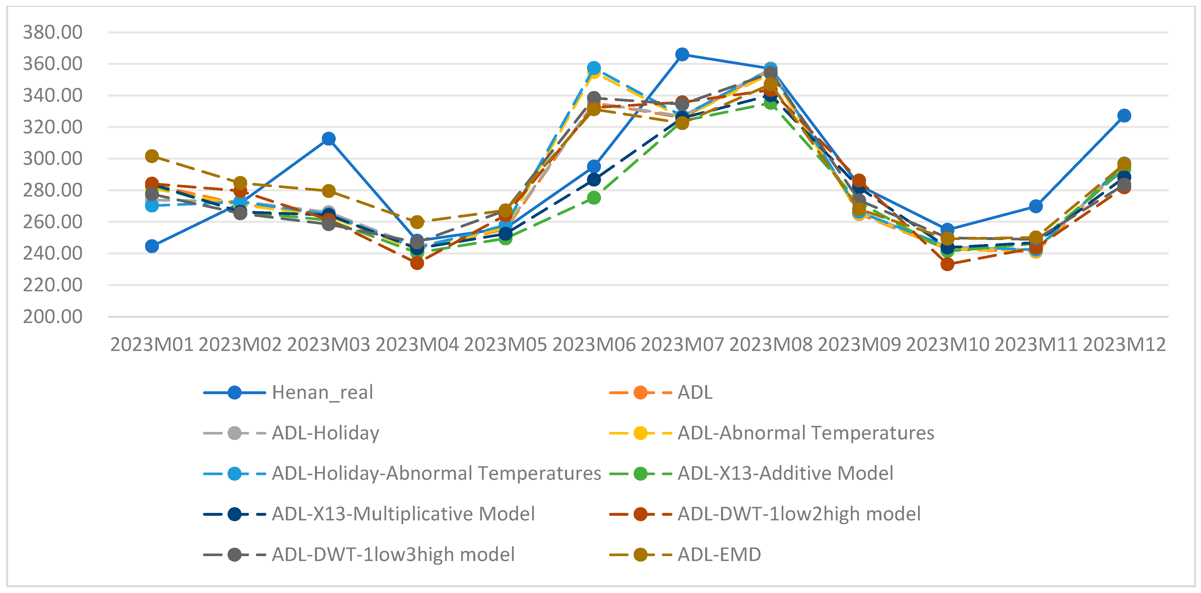
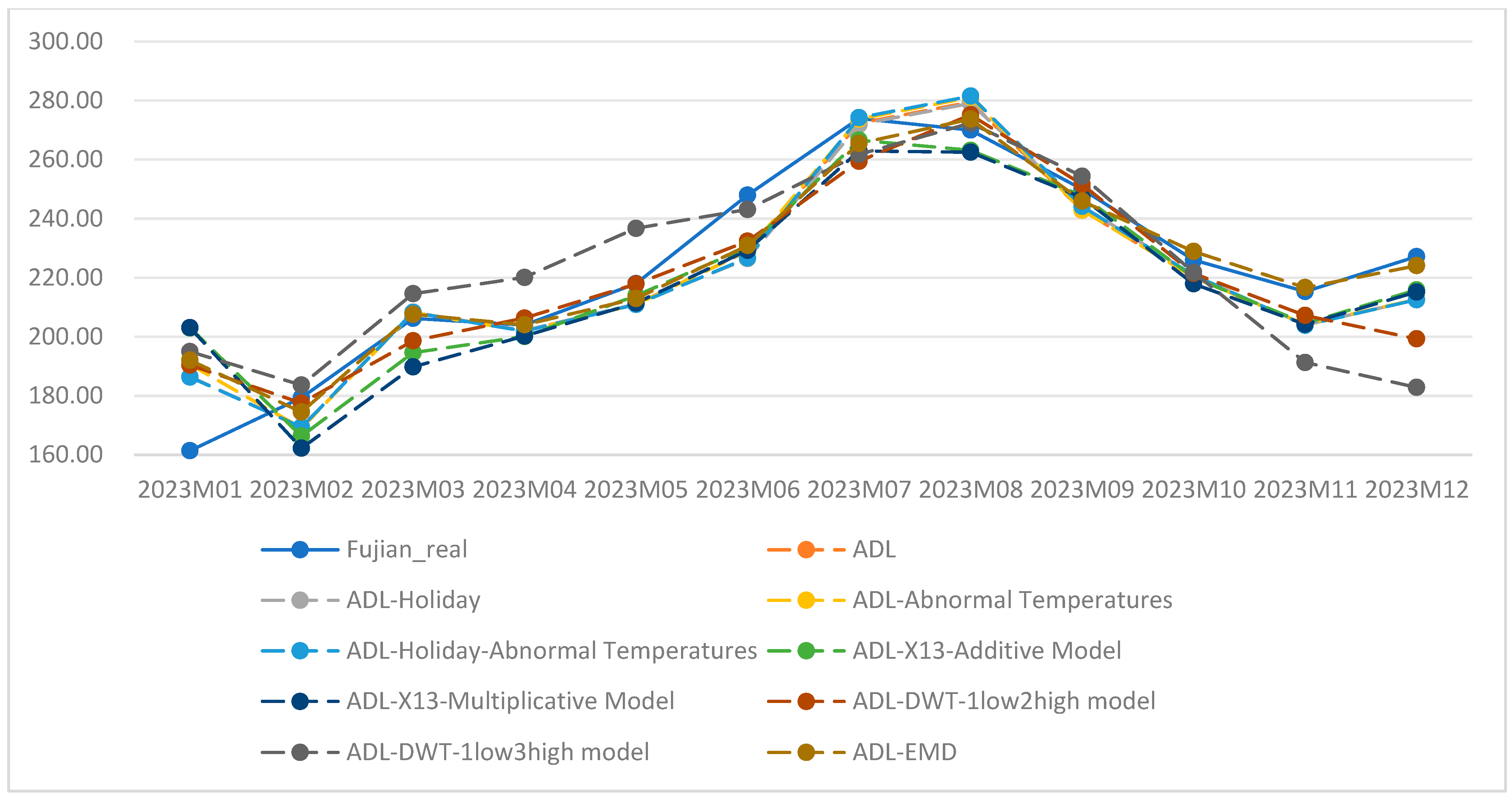
In this section, we construct an ADL model using electricity consumption as the exogenous variable. The ADL model was applied to forecast electricity sales, considering three scenarios: (1) incorporating holidays, (2) incorporating abnormal temperature, and (3) incorporating both holidays and abnormal temperature. As a result, we obtained four models: the basic ADL model, ADL model with holidays, ADL model with abnormal temperature, and ADL model with both holidays and abnormal temperature.
Without using feature decomposition, the monthly electricity sales forecast for the national grid region, Henan Province, and Fujian Province in 2023 was made 12 times throughout the year, as per the forecasting requirements outlined in Section 3.4. It should be noted that due to the difficulty of obtaining abnormal temperature data for the national grid region, we only considered the ADL model and the ADL model with holidays for this region.
When using the ADL model combined with different feature decomposition methods, we decomposed both electricity sales and electricity consumption, then used the corresponding decomposed components to construct the ADL models for forecasting. After synthesizing the predicted results from the decomposed components, the final electricity sales forecast was obtained. Since the X-13 decomposition included both multiplicative and additive models, we constructed the ADL-X13 additive model and ADL-X13 multiplicative model based on the corresponding decomposition methods. For DWT decomposition, since X13 decomposition extracted the trend-cycle (TC), seasonal (S), and irregular (I) components, we considered two decomposition levels: two layers (with high-frequency components) and three layers (with high-frequency components). Similarly to the seasonal adjustment decomposition, we constructed ADL-DWT (one low-frequency component and two high-frequency components) and ADL-DWT (one low-frequency component and three high-frequency components) models. For EMD, since the automatic decomposition resulted in five components (one low-frequency component and four high-frequency components), we merged the four high-frequency components based on their similarity, resulting in three components. Thus, we constructed the ADL-EMD model (three components) for forecasting electricity sales. In total, based on different feature decomposition methods, we created five forecasting models using the ADL model.
The following tables and figures (Table 1, Table 2 and Table 3 and Figure 1, Figure 2 and Figure 3) present the relative error results of the 12 annual forecasts for 2023, comparing the 5 forecasting models under feature decomposition methods, as well as the ADL models without feature decomposition for the national grid region, Henan Province, and Fujian Province.

4.2. Comparison of Electricity Sales Forecasting Results Using SARIMAX Model with Different Feature Decomposition Methods

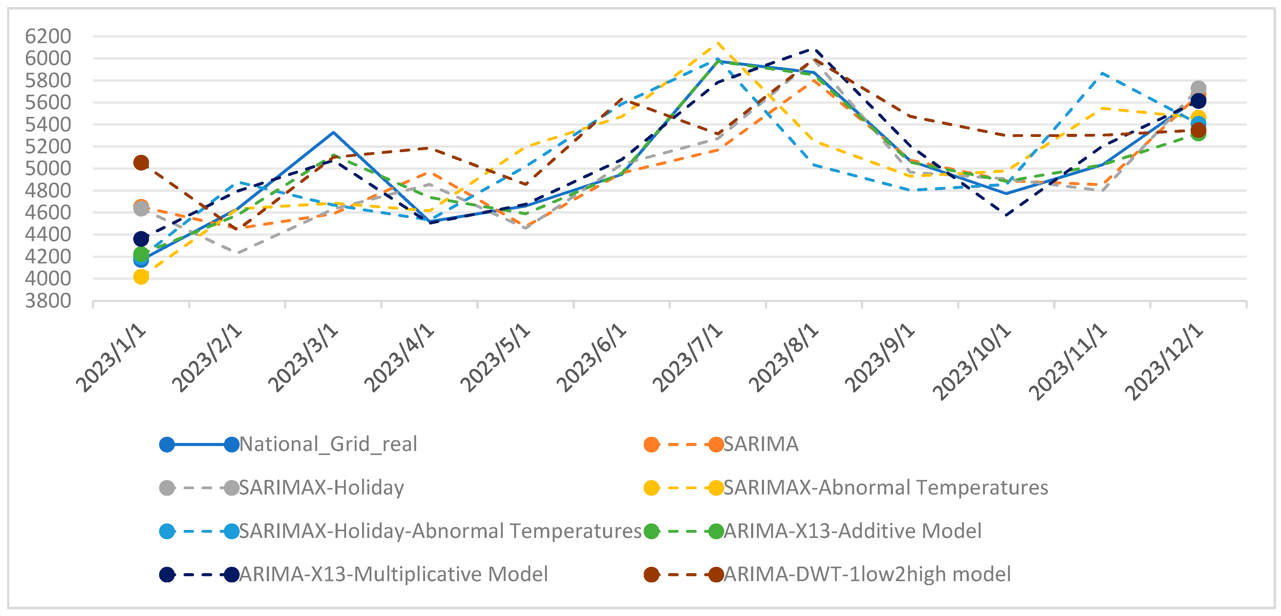
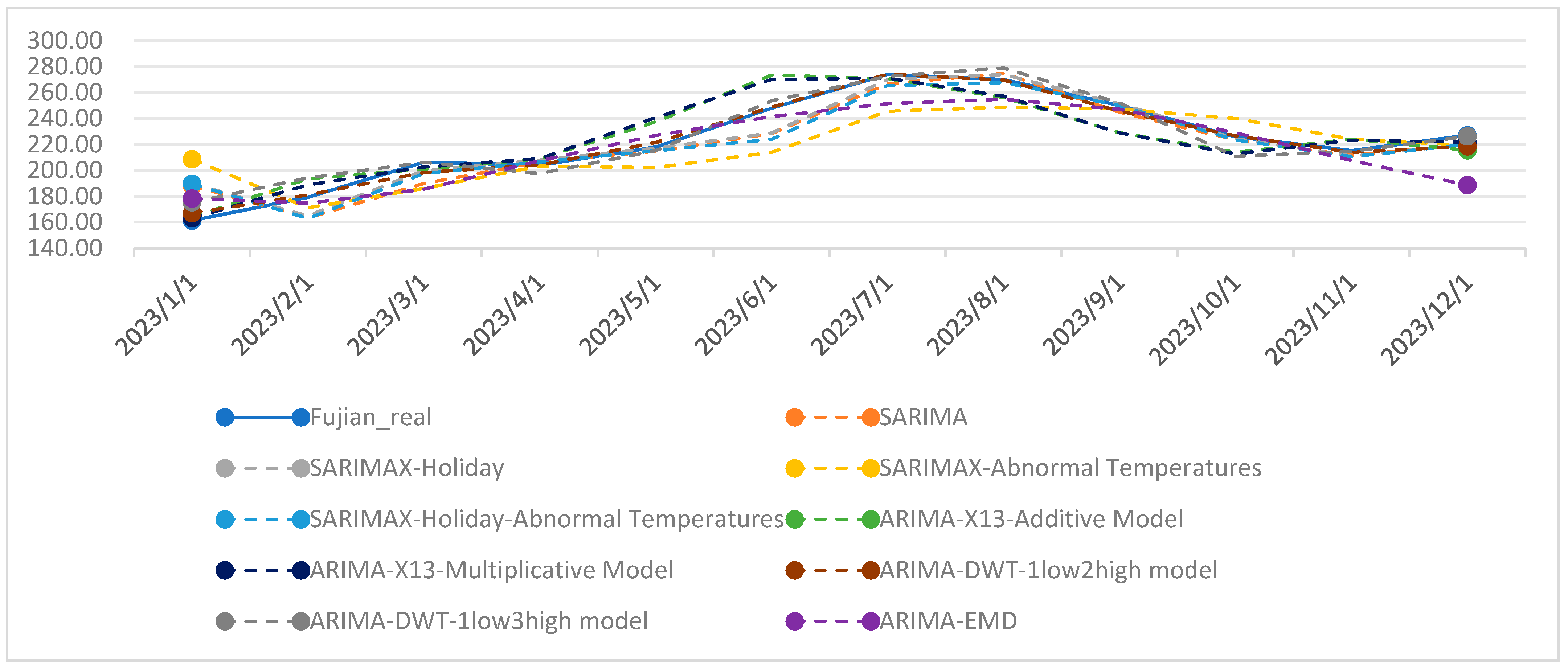
For the SARIMAX model, we began by directly applying the SARIMA model to forecast electricity sales without feature decomposition. Next, we incorporated holiday effects as exogenous variables XXX to construct the SARIMAX-holiday model for forecasting. We then introduced abnormal temperature effects as exogenous variables XXX and built the SARIMAX-abnormal temperature model. Finally, we included both holidays and abnormal temperature effects as exogenous variables to construct the SARIMAX-holiday-abnormal temperature model for forecasting.
The forecasting targets remained the national grid region, Henan Province, and Fujian Province for the year 2023, with 12 monthly forecasts performed for each sample region. Similarly to the previous section, due to the difficulty in obtaining abnormal temperature data for the national grid region, only the SARIMA model and the SARIMAX-holiday model were considered for this region.
When using the SARIMAX model combined with different feature decomposition methods, the decomposed components were typically predicted using the ARIMA model. Specifically, for X13 decomposition, we constructed both the ARIMA-X13 additive model and ARIMA-X13 multiplicative model. For DWT decomposition, we created the ARIMA-DWT (one low-frequency component and two high-frequency components) and ARIMA-DWT (one low-frequency component and three high-frequency components) models. For EMD, we constructed the ARIMA-EMD model (three components). Thus, based on the different feature decomposition methods, we constructed five forecasting models using the SARIMAX model in combination with ARIMA.
The following tables and figures (Table 4, Table 5 and Table 6 and Figure 4, Figure 5 and Figure 6) show the relative error results of the 12 annual forecasts for 2023 for each model under feature decomposition methods, as well as the SARIMAX models without feature decomposition for the national grid region, Henan Province, and Fujian Province.

4.3. Comparison of Electricity Sales Forecasting Results Using LSTM Model with Different Feature Decomposition Methods

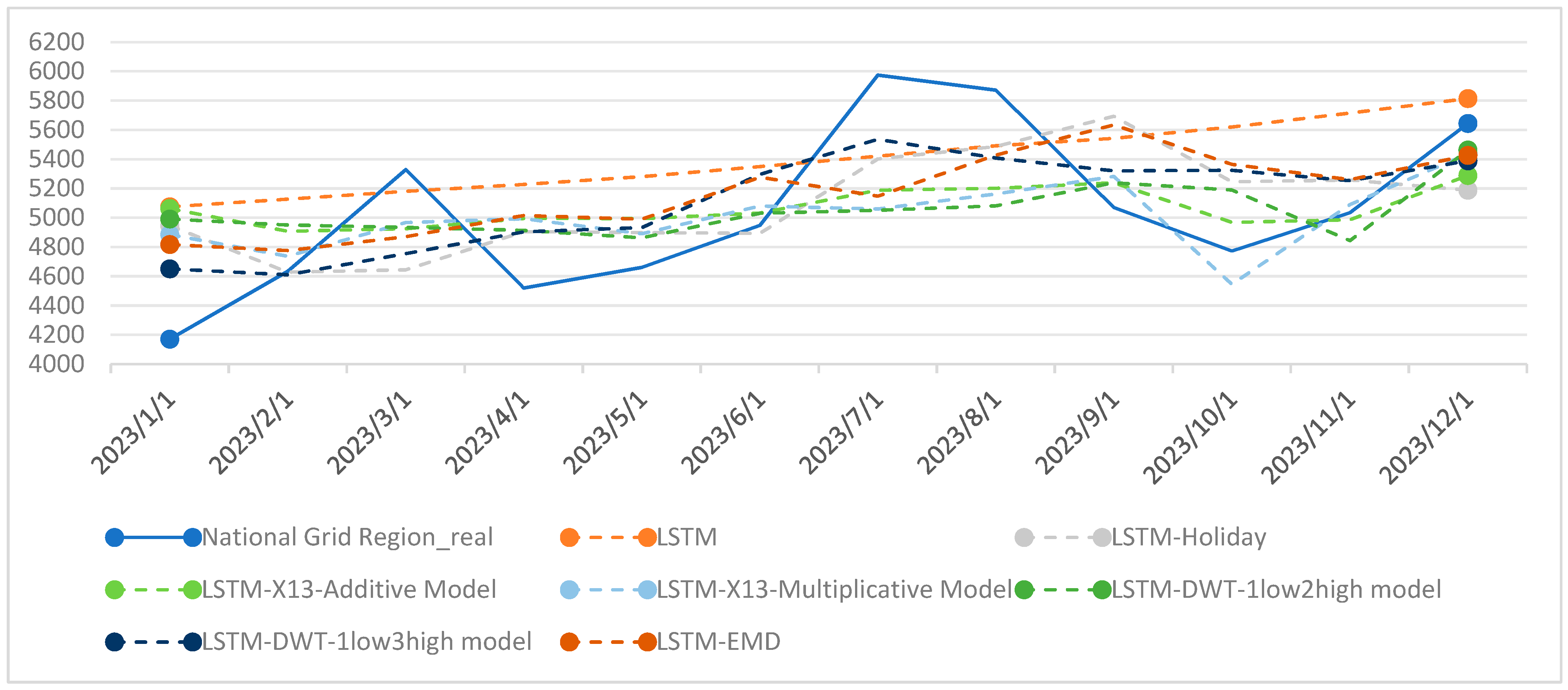
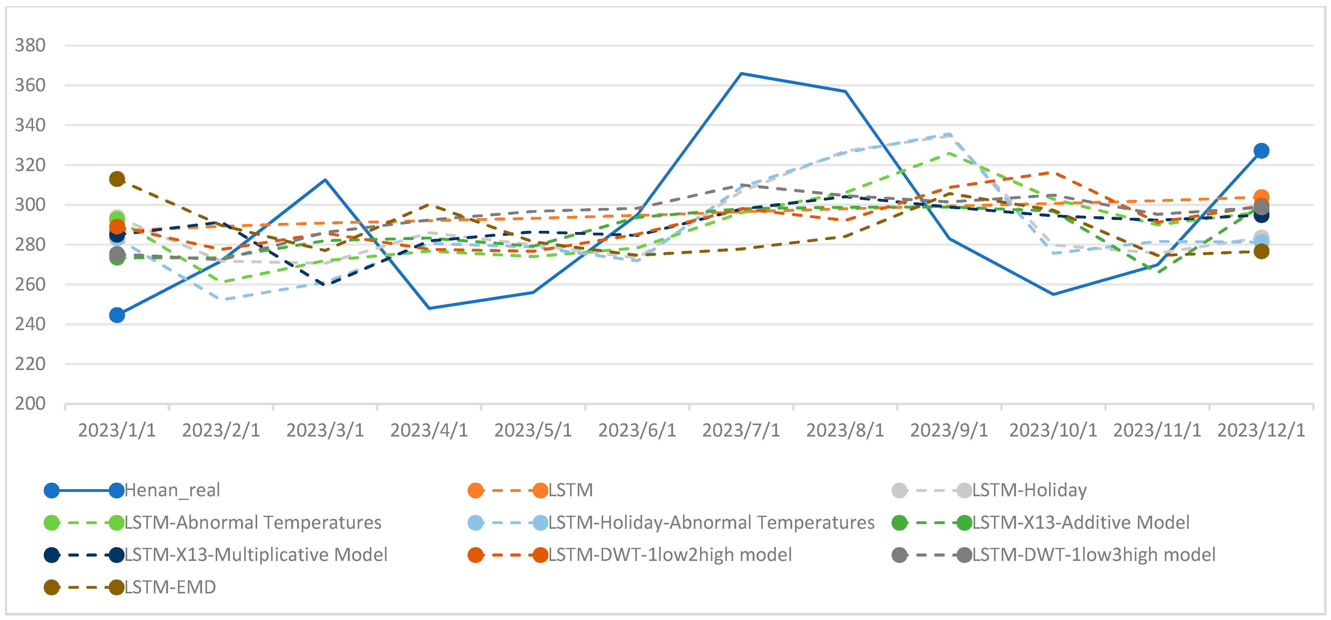
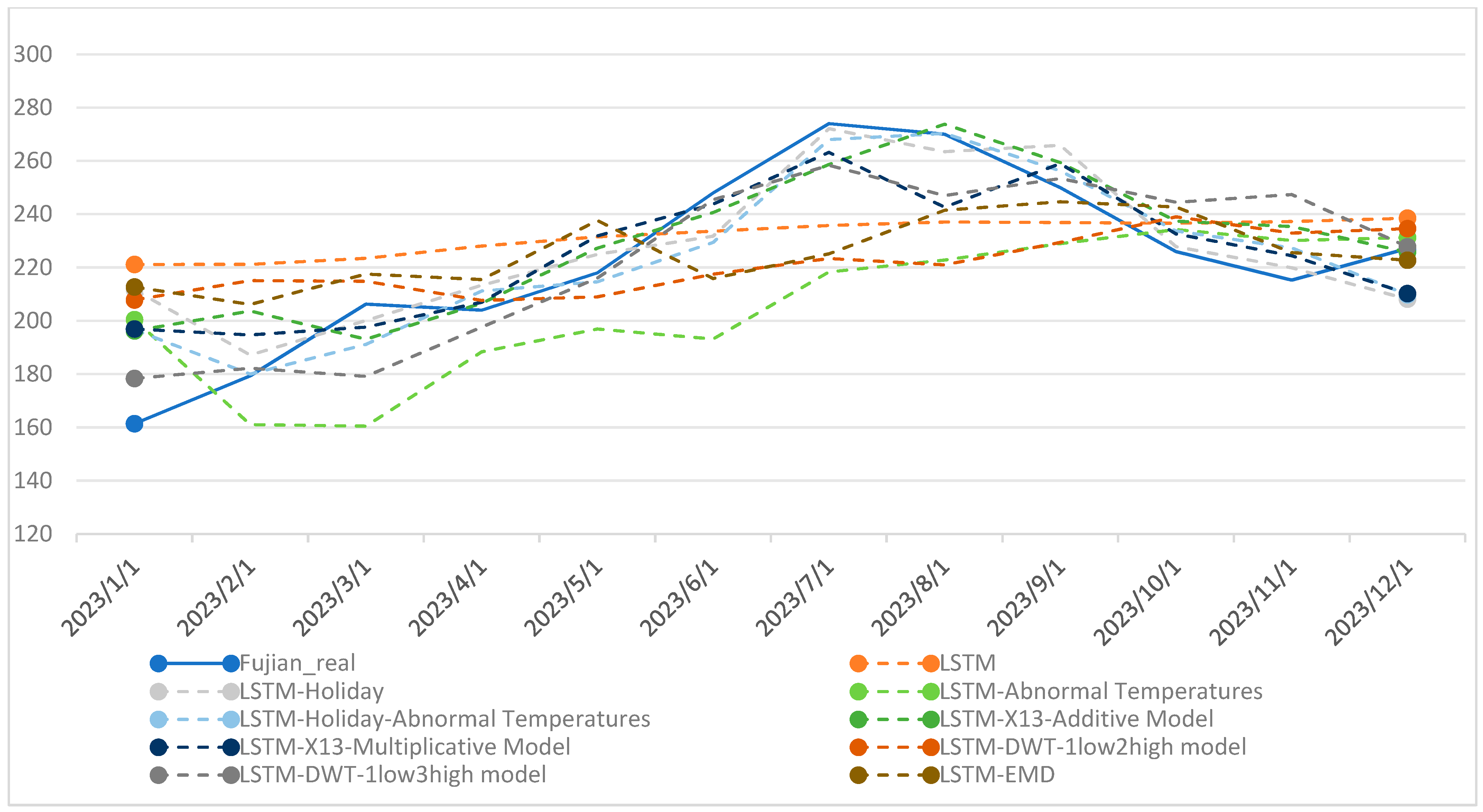
For the LSTM model, similarly to Section 4.1 and Section 4.2, without considering feature decomposition, we constructed the following four types of LSTM models: LSTM model only, LSTM model with exogenous variables including holidays, LSTM model with exogenous variables including abnormal temperature, and LSTM model with exogenous variables including abnormal temperature and holidays.
When applying different feature decomposition methods to the LSTM model, similarly to Section 4.1 and Section 4.2, we constructed the following five models: LSTM-X13 additive model, LSTM-X13 multiplicative model, LSTM-DWT (one low-frequency component and two high-frequency components) model, LSTM-DWT (one low-frequency component and three high-frequency components) model, and LSTM-EMD model (three components).
The following tables and figures (Table 7, Table 8 and Table 9 and Figure 7, Figure 8 and Figure 9) show the relative error results of the 12 annual forecasts for 2023 for each model under feature decomposition methods, as well as the LSTM models without feature decomposition for the national grid region, Henan Province, and Fujian Province.
In order to better compare and analyze the screening results of various models in the three regions, we counted the total number of prediction models and the number of models that met the prediction requirements for each category in each region. The results are shown in Table 10. From the table, it can be seen that firstly, at the model level, the ADL class models have the highest number of models that can meet the prediction requirements, which is 12. Secondly, from a regional perspective, Fujian Province has the highest number of models selected to meet forecasting requirements, at 8.
Taking the prediction results of the seven types of ADL models in the national grid region as an example, we present a graphical display of the prediction errors. Figure 10 shows the relative errors of the seven types of models in 12 annual predictions from January to December 2023. The prediction results of four models (ADL-Abnormal Temperature, ADL-X13-Additive, ADL-X13-Multiplicative, and ADL-DWT-1low2high) meet the requirement of an error of less than 2%.

5. Conclusions and Future Work

This article introduces three types of basic prediction models, namely the ADL model, SARIMAX model, and LSTM model, and for the first time achieves a comparative study of three different feature decomposition methods (X13 decomposition, DWT decomposition, and EMD) in electricity sales prediction. Based on the comparison of the forecasting results for electricity sales in the three sample regions using different prediction models, the following conclusions can be drawn:
Overall, forecasting results based on feature decomposition outperform those of direct forecasting without decomposition. This indicates the importance of feature decomposition in electricity sales forecasting. In the comparison of the three different feature decomposition methods, the optimal decomposition method differs depending on the sample region. For regions with high volatility in electricity sales, EMD is recommended, while for regions with relatively stable electricity sales, DWT decomposition should be preferred. When combined with feature decomposition, the ADL model generally performed better than the SARIMAX model, and the SARIMAX model performed better than the LSTM model. In terms of model selection for the sample regions, for the national grid region, five forecasting models meet the criterion of “annual forecasting error for each of the 12 monthly forecasts being below 2%”: the ADL-X13 additive model, ADL-DWT (one low-frequency and two high-frequency components) model, ADL-DWT (one low-frequency and three high-frequency components) model, ADL-EMD model (three components), and ARIMA-DWT (one low-frequency and three high-frequency components) model. For Henan Province, only two models meet the standard: the ADL-EMD model (three components) and LSTM model. For Fujian Province, seven models meet the criterion, including the ADL model, ADL-holiday model, ADL-abnormal temperature model, ADL-holiday-abnormal temperature model, ADL-DWT (one low-frequency and two high-frequency components) model, ADL-DWT (one low-frequency and three high-frequency components) model, and ADL-EMD model (three components). Finally, it is worth noting that the Henan Province data exhibited higher volatility than that of Fujian Province, which explains the differing number of models meeting the evaluation standard in these regions.
When applying the research results of this article to the actual operation of predicting electricity sales in other regions, based on our research experience, the following suggestions are given: Firstly, if conditions permit, try to collect sequence data of both electricity sales and electricity consumption indicators simultaneously to provide support for constructing ADL models. Secondly, when combining feature decomposition methods with basic prediction methods, it is recommended to refer to Section 4.1, Section 4.2 and Section 4.3 of this article as much as possible. Thirdly, when implementing different feature decomposition methods, it is recommended to refer to the decomposition forms given in the headers of Table 1, Table 2, Table 3, Table 4, Table 5, Table 6, Table 7, Table 8 and Table 9 in this article. Fourthly, in terms of specific code implementation, it is recommended to use Python to implement all algorithms.
For future research, we propose the following three directions. Firstly, expand the sample regions and further validate the conclusions drawn from this study. Secondly, incorporate ensemble forecasting methods and combine the models selected for each sample region to assess whether combining forecasts yields more stable and robust results than using individual models. Thirdly, in future forecasting of electricity sales across more sample regions, consider comparing models based on their adaptability to the volatility of electricity sales in different regions, and further investigate the effectiveness of models under various data characteristics.

Author Contributions

Conceptualization, S.C. and Y.Z.; methodology, X.M. and X.Y.; software, Y.Z.; validation, S.C., H.J. and J.S.; formal analysis, Y.Z.; investigation, S.C., H.J. and J.S.; resources, X.Y.; data curation, X.Y.; writing—original draft preparation, S.C., H.J. and J.S.; writing—review and editing, S.C., H.J. and J.S.; visualization, H.J.; supervision, H.J. and J.S.; project administration, J.S.; funding acquisition, J.S. All authors have read and agreed to the published version of the manuscript.

Funding

This paper is funded by the Research Project on Electricity Sales Prediction Technology and Its Application Based on Dynamic Time Series Analysis and Multi-dimensional Feature Engineering Processing of State Grid Big Data Center (SGSJ0000NYJS2500044).

Institutional Review Board Statement

Not applicable.

Informed Consent Statement

Not applicable.

Data Availability Statement

The original contributions presented in this study are included in the article. Further inquiries can be directed to the corresponding author(s).

Conflicts of Interest

Author Shichong Chen, Yushu Zhang, and Xiaoteng Ma were employed by State Grid Information & Telecommunication Center (Big Data Center). The remaining authors declare that the research was conducted in the absence of any commercial or financial relationships that could be construed as a potential conflict of interest.

Abbreviations

The following abbreviations are used in this manuscript:
AcronymFull TermDefinition
X13X-13-ARIMA-SEATSSeasonal adjustment method combining X-11 and SEATS with TRAMO-style preprocessing; decomposes a series into Trend, Cycle, Seasonal, and Irregular components.
X-11X-11 Seasonal AdjustmentClassic seasonal adjustment filter; a core module within X13.
SEATSSignal Extraction in ARIMA Time SeriesARIMA-based signal extraction seasonal adjustment method used within X13.
TRAMO/TRAMOSTime Series Regression with ARIMA Noise, Missing Observations and OutliersPre-adjustment approach (regression with ARIMA noise) for outliers and missing values, used by X13.
RegARIMARegression with ARIMA ErrorsRegression model with ARIMA error structure used in X13 preprocessing to remove deterministic effects.
EMDEmpirical Mode DecompositionAdaptive decomposition of a signal into several Intrinsic Mode Functions (IMFs) and a residual trend.
IMF/IMFsIntrinsic Mode Function(s)Oscillatory components produced by EMD that capture different characteristic scales.
DWTDiscrete Wavelet TransformMulti-scale wavelet decomposition into low-frequency (trend) and high-frequency (detail/noise) components.
ADLAutoregressive Distributed LagTime-series regression with lags of the dependent variable and current/lagged exogenous variables.
ARIMAAutoregressive Integrated Moving AverageClassical time-series model combining AR, differencing (I), and MA components.
SARIMASeasonal ARIMAARIMA with seasonal terms; seasonal parameters are P (SAR), D (seasonal differencing), Q (SMA), and S (seasonal period).
SARIMAXSeasonal ARIMA with eXogenous RegressorsSARIMA model extended to include exogenous variables X.
LSTMLong Short-Term MemoryRecurrent neural network architecture designed to capture long-term temporal dependencies.
RNNRecurrent Neural NetworkNeural network class for sequence modeling with recurrent connections.
ReLURectified Linear UnitActivation function max(0, x) commonly used to mitigate vanishing gradients.
TCTrend–CycleCombined trend and cycle component (often denoted TC in X13 outputs).
T/C/S/ITrend/Cycle/Seasonal/IrregularFour components of seasonal adjustment decomposition.
SISeasonal differencing orderOrder of seasonal differencing in SARIMA/SARIMAX.
NOAANational Oceanic and Atmospheric AdministrationUS federal agency providing meteorological data (temperature series source in the paper).
GM(1,1)Grey Model (1,1)Univariate first-order grey forecasting model.
RBF (NN)Radial Basis Function Neural NetworkNeural network using radial basis functions as activation units.
BP (NN)Backpropagation Neural NetworkFeedforward neural network trained via backpropagation.
LSSVMLeast Squares Support Vector MachineLS-SVM variant using least squares cost for regression/classification.
SDStandard Deviation (EMD stopping criterion)Stopping criterion in EMD sifting (e.g., SD ≤ 0.2–0.3).
HWHolt–WintersSeasonal exponential smoothing model (mentioned as a comparative method).

References

  1. Gao, L.; Liang, S.; Chen, S.; Li, S. Short-term load forecasting method for distribution networks based on multi-level load clustering and decoupling mechanisms. Power Syst. Its Autom. J. 2021, 33, e0300229. [Google Scholar]
  2. Zhuang, J.; Li, K.; Liu, Z.; Cheng, X. Research on monthly electricity sales forecasting based on seasonal adjustment and regression analysis. Econ. Res. Guide 2018, 19, 181–186. [Google Scholar]
  3. Zhuang, J.; Li, K.; Liu, Z.; Liu, R. Study of monthly electricity sales forecasting based on seasonal adjustment and multi-factor correction method. In Proceedings of the 30th Chinese Control and Decision Conference, Shenyang, China, 9–11 June 2018; pp. 1–6. [Google Scholar]
  4. Liu, J.; Zhao, J.; Chen, Y.; Fang, X.; Liu, Y.; Wang, S.; Chen, Y.; Ou, H. Correction method for electricity sales forecasting results considering the impact of the Spring Festival. In 2018 Power Industry Informationization Annual Conference Proceedings; China Electric Power Engineering Society: Beijing, China, 2018; pp. 424–425. [Google Scholar]
  5. Lang, J.; Jin, J.; Li, R.; Wang, Y.; Shen, B. Analysis of the impact of special events on monthly electricity sales and its forecasting. Power Big Data 2018, 21, 43–48. [Google Scholar]
  6. Qi, Z. Research on electricity sales forecasting based on LSTM deep network. China New Technol. New Prod. 2023, 23, 133–135. [Google Scholar] [CrossRef]
  7. Klyuev, R.V.; Morgoev, I.D.; Morgoeva, A.D.; Gavrina, O.A.; Martyushev, N.V.; Efremenkov, E.A.; Mengxu, Q. Methods of forecasting electric energy consumption: A literature review. Energies 2022, 15, 8919. [Google Scholar] [CrossRef]
  8. Salkuti, S.R. Short-term electrical load forecasting using radial basis function neural networks considering weather factors. Electr. Eng. 2018, 100, 1985–1995. [Google Scholar] [CrossRef]
  9. Deng, F.; Si, J.; Deng, Z.; Yu, B.; Li, H.; Jin, M. QPSO-LSTM Based Electricity Sales Forecasting Model. In Proceedings of the 2024 6th Asia Energy and Electrical Engineering Symposium (AEEES), Chengdu, China, 28–31 March 2024; pp. 1347–1352. [Google Scholar] [CrossRef]
  10. Gnatyuk, V.I.; Kivchun, O.R.; Morozov, D.G. Electric consumption predictions of socio-economic systems based on the ranked values. Mar. Intellect. Technol. 2020, 4, 107–111. [Google Scholar]
  11. Li, W.; Li, X.; Fan, P.; Zhang, H. Regional electricity sales forecasting based on multi-head self-attention mechanism and LSTM network. Power Demand Side Manag. 2025, 27, 67–73. [Google Scholar]
  12. Yang, L.; Wu, Y.; Zhang, C.; Liu, C.; Jiang, B.; Zhang, P. Improved least squares support vector machine electricity forecasting algorithm. Power Grid Clean Energy 2017, 33, 71–76. [Google Scholar]
  13. Sun, W.; Liu, X.; He, Q. Monthly industry electricity sales forecasting based on similar months and Elman neural network. Power Demand Side Manag. 2022, 24, 53–58. [Google Scholar]
  14. Ma, X.; Sun, C.; Wang, W.; Zhao, R.; Chen, P.; Wu, B. Research on proxy electricity purchase forecasting considering meteorological and special event impacts. Power Inf. Commun. Technol. 2025, 23, 25–32. [Google Scholar] [CrossRef]
  15. Wei, T.; Tang, K. Classification and monthly electricity forecasting based on BP neural network and regression analysis. Electr. Ind. 2023, 11, 74–78. [Google Scholar]
  16. Zhang, L.; Ji, T.; Liu, J. Monthly electricity forecasting considering sub-sectors and multiple influencing factors. Guangdong Electr. Power 2023, 36, 30–39. [Google Scholar]
  17. Yao, L.X.; Liu, X.Q. Monthly load combination forecasting based on wavelet analysis. Power Syst. Technol. 2007, 31, 65–68. [Google Scholar]
  18. Zhang, T.; Zhu, J. Wavelet regression analysis method in short-term power system load forecasting. J. Harbin Univ. Sci. Technol. 2008, 1, 74–76. [Google Scholar]
  19. Meng, M.; Niu, D.; Sun, W. Forecasting monthly electric energy consumption using feature extraction. Energies 2011, 4, 1495–1507. [Google Scholar] [CrossRef]
  20. Fan, J.; Feng, H.; Niu, D. Monthly electricity sales forecasting based on wavelet analysis and GM-ARIMA model. J. North China Electr. Power Univ. (Nat. Sci. Ed.) 2015, 42, 101–105. [Google Scholar]
  21. Asadpour, M.; Pourhaji, N.; Ahmadian, A. Electricity price and load demand forecasting using an adaptive hybrid BiLSTM model based on wavelet transform technique and Pareto optimization: An application in the smart cities. J. Energy Manag. Technol. 2024, 8, 178–195. [Google Scholar]
  22. Buratto, W.G.; Muniz, R.N.; Nied, A.; Barros, C.F.d.O.; Cardoso, R.; Gonzalez, G.V. Wavelet CNN-LSTM time series forecasting of electricity power generation considering biomass thermal systems. IET Gener. Transm. Distrib. 2024, 18, 3654–3663. [Google Scholar] [CrossRef]
  23. Kumar, M.; Kumar, J. Impact of Coiflet Wavelet Decomposition on Forecasting Accuracy: Shifts in ARIMA and Exponential Smoothing Performance. Metall. Mater. Eng. 2025, 31, 177–192. [Google Scholar] [CrossRef]
  24. Yan, W.; Cheng, C.; Xue, B.; Li, D.; Chen, F.; Wang, S. Monthly electricity sales forecasting method combining X12 multiplicative model and ARIMA model. Power Syst. Its Autom. J. 2016, 28, 74–80. [Google Scholar]
  25. Wang, A.; Wang, D.; Ye, J. Monthly electricity sales forecasting model based on factorization machine. J. Tianjin Vocat. Tech. Norm. Univ. 2020, 30, 42–47. [Google Scholar] [CrossRef]
  26. Mei, X.; Cao, W.; Wang, J. Monthly electricity sales forecasting method for large power customers based on empirical mode decomposition and ARIMA model. Autom. Technol. Appl. 2025, 44, 13–17. Available online: http://kns.cnki.net/kcms/detail/23.1474.TP.20241218.0957.008.html (accessed on 18 December 2024). [CrossRef]
  27. Wu, H.; Xu, J.; Wang, J.; Long, M. Autoformer: Decomposition Transformers with Auto-Correlation for Long-Term Series Forecasting. In 35th Conference on Neural Information Processing Systems (NeurIPS 2021); Curran Associates Inc.: Red Hook, NY, USA, 2021. [Google Scholar] [CrossRef]
  28. Liu, Y.; Zhang, H.; Li, C.; Huang, X.; Wang, J.; Long, M. Timer: Generative Pre-trained Transformers Are Large Time Series Models. arXiv 2024, arXiv:2402.02368. [Google Scholar] [CrossRef]
  29. Liu, Y.; Qin, G.; Huang, X.; Wang, J.; Long, M. Timer-XL: Long-Context Transformers for Unified Time Series Forecasting. arXiv 2025, arXiv:2410.04803. [Google Scholar] [CrossRef]
  30. Guo, Y. Application of wavelet transform in signal denoising based on LabVIEW. Intern. Combust. Engine Parts 2017, 18, 144–145. [Google Scholar]
  31. Huang, N.E.; Shen, Z.; Long, S.R.; Wu, M.C.; Shih, H.H.; Zheng, Q.; Yen, N.-C.; Tung, C.C.; Liu, H.H. The empirical mode decomposition and the Hilbert spectrum for nonlinear and non-stationary time series analysis. Proc. R. Soc. A 1998, 454, 903–995. [Google Scholar] [CrossRef]
  32. Chen, L.; Chi, Y.; Guan, Y.; Fan, J. A hybrid attention-based EMD-LSTM model for financial time series prediction. In Proceedings of the 2019 International Conference on Artificial Intelligence and Big Data, Chengdu, China, 25–28 May 2019; pp. 113–118. [Google Scholar]
  33. Taylor, S.J.; Letham, B. Forecasting at Scale. Am. Stat. 2018, 72, 37–45. [Google Scholar] [CrossRef]
  34. Shi, J.; Tang, H.; Zhou, Q.; Han, L.; Hao, R. High frequency measurement of carbon emissions based on power big data: A case study of Chinese Qinghai province. Sci. Total Environ. 2023, 902, 166075. [Google Scholar] [CrossRef] [PubMed]
  35. Hochreiter, S.; Schmidhuber, J. Long Short-Term Memory. Neural Comput. 1997, 9, 1735–1780. [Google Scholar] [CrossRef]
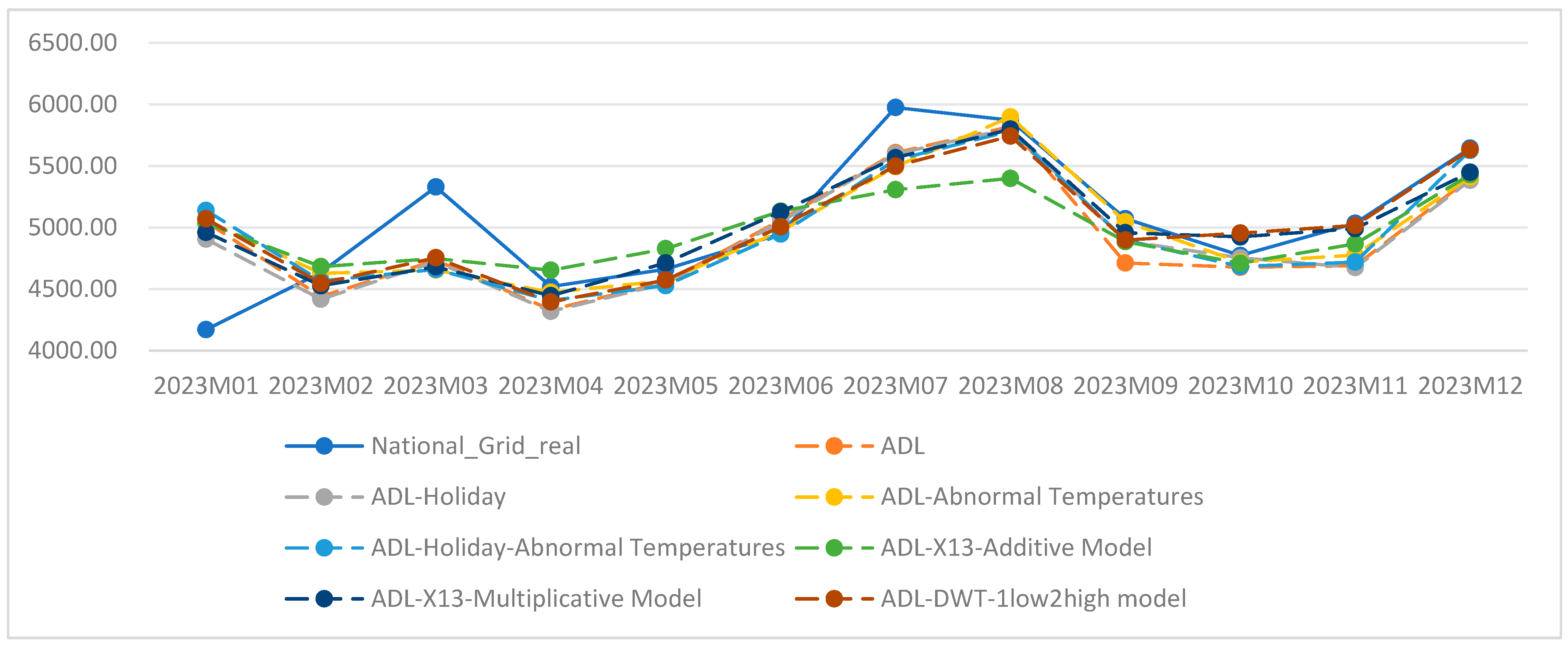
Figure 1. Forecasting results using ADL model with different feature decomposition methods for national grid region (monthly).
Energies 18 05352 g001
Figure 2. Forecasting results using ADL model with different feature decomposition methods for Henan Province (monthly).
Energies 18 05352 g002
Figure 3. Forecasting results using ADL model with different feature decomposition methods for Fujian Province (monthly).
Energies 18 05352 g003
Figure 4. Forecasting results using SARIMAX model with different feature decomposition methods for national grid region (monthly).
Energies 18 05352 g004
Figure 5. Forecasting results using SARIMAX model with different feature decomposition methods for Henan Province (monthly).
Energies 18 05352 g005
Figure 6. Forecasting results using SARIMAX model with different feature decomposition methods for Fujian Province (monthly).
Energies 18 05352 g006
Figure 7. Forecasting results using LSTM model with different feature decomposition methods for national grid region (monthly).
Energies 18 05352 g007
Figure 8. Forecasting results using LSTM model with different feature decomposition methods for Henan Province (monthly).
Energies 18 05352 g008
Figure 9. Forecasting results using LSTM model with different feature decomposition methods for Fujian Province (monthly).
Energies 18 05352 g009
Figure 10. Annual forecast errors of seven different ADL models.
Energies 18 05352 g010
Table 1. Forecasting results using ADL model with different feature decomposition methods for national grid region.
Forecast HorizonADLADL-HolidayADL-Abnormal TemperaturesADL-Holiday-Abnormal TemperaturesADL-X13-Additive ModelADL-X13-Multiplicative ModelADL-DWT-1low2high ModelADL-DWT-1low3high ModelADL-EMD
122.62%2.76%N/AN/A1.57%2.01%1.53%1.04%0.72%
113.03%3.07%N/AN/A1.65%2.10%1.71%1.10%0.83%
102.97%3.00%N/AN/A1.66%2.09%1.77%1.07%0.84%
92.77%2.79%N/AN/A1.61%2.02%1.75%0.97%0.80%
82.72%2.74%N/AN/A1.61%1.98%1.76%0.92%0.80%
72.70%2.71%N/AN/A1.60%1.95%1.76%0.87%0.81%
62.73%2.74%N/AN/A1.60%1.93%1.75%0.84%0.84%
52.63%2.64%N/AN/A1.58%1.90%1.68%0.80%0.86%
42.62%2.63%N/AN/A1.57%1.89%1.66%0.81%0.87%
32.59%2.61%N/AN/A1.56%1.87%1.61%0.81%0.87%
22.58%2.61%N/AN/A1.56%1.87%1.60%0.82%0.89%
12.57%2.60%N/AN/A1.55%1.86%1.58%0.81%0.89%
Number of Errors Exceeding 2%1212N/AN/A04000
Note: Here N/A means that the relative model cannot be used due to the difficulty of obtaining abnormal temperature data for the national grid region.
Table 2. Forecasting results using ADL model with different feature decomposition methods for Henan Province.
Forecast
Horizon
ADLADL-HolidayADL-Abnormal
Temperatures
ADL-Holiday-Abnormal TemperaturesADL-X13-Additive ModelADL-X13-Multiplicative ModelADL-DWT-1low2high ModelADL-DWT-1low3high ModelADL-EMD
122.99%3.07%2.47%2.39%6.05%4.84%3.07%2.85%0.12%
113.25%3.20%2.60%2.42%6.09%4.93%3.23%2.84%0.34%
103.25%3.21%2.60%2.42%6.06%4.90%3.27%2.79%0.41%
93.04%3.00%2.45%2.27%5.94%4.80%3.19%2.69%0.44%
83.02%2.99%2.44%2.26%5.91%4.77%3.14%2.64%0.52%
73.02%2.99%2.44%2.27%5.88%4.76%3.10%2.64%0.59%
63.24%3.17%2.81%2.67%5.81%4.74%3.10%2.68%0.69%
53.09%3.01%2.65%2.52%5.76%4.71%3.12%2.63%0.74%
43.08%3.01%2.65%2.52%5.73%4.70%3.14%2.60%0.92%
33.07%2.99%2.63%2.49%5.70%4.69%3.09%2.59%0.85%
23.06%2.99%2.62%2.49%5.67%4.67%3.08%2.55%0.81%
13.05%2.98%2.60%2.47%5.66%4.66%3.05%2.51%0.81%
Number of
Errors
Exceeding 2%
12121212121212120
Table 3. Forecasting results using ADL model with different feature decomposition methods for Fujian Province.
Forecast
Horizon
ADLADL-HolidayADL-Abnormal TemperaturesADL-Holiday-Abnormal
Temperatures
ADL-X13-Additive ModelADL-X13-Multiplicative ModelADL-DWT-1low2high ModelADL-DWT-1low3high ModelADL-EMD
121.42%1.62%1.40%1.55%2.22%3.26%1.62%−0.29%−0.20%
111.63%1.79%1.56%1.67%2.26%3.28%1.72%−0.11%−0.09%
101.58%1.74%1.50%1.62%2.26%3.18%1.73%0.01%−0.01%
91.59%1.76%1.52%1.63%2.24%3.05%1.70%0.07%0.03%
81.58%1.75%1.51%1.62%2.19%2.97%1.66%0.14%0.08%
71.54%1.71%1.48%1.59%2.13%2.91%1.65%0.18%0.11%
61.42%1.61%1.32%1.45%2.09%2.85%1.62%0.18%0.08%
51.41%1.59%1.31%1.45%2.06%2.81%1.60%0.18%0.05%
41.45%1.63%1.34%1.48%2.03%2.79%1.61%0.18%0.07%
31.43%1.62%1.32%1.46%2.00%2.76%1.61%0.21%0.08%
21.42%1.61%1.31%1.45%1.99%2.75%1.59%0.16%0.09%
11.42%1.61%1.31%1.45%1.98%2.74%1.57%0.07%0.10%
Number of
Errors
Exceeding 2%
00001012000
Table 4. Forecasting results using SARIMAX model with different feature decomposition methods for national grid region.
Forecast
Horizon
SARIMASARIMAX-HolidaySARIMAX-Abnormal TemperaturesSARIMAX-Holiday-Abnormal
Temperatures
ARIMA-X13-Additive ModelARIMA-X13-Multiplicative ModelARIMA-DWT-1low2high ModelARIMA-DWT-1low3high ModelARIMA-EMD
12−3.64%−4.08%N/AN/A−12.07%−3.31%−3.18%0.52%4.03%
11−5.09%−5.83%N/AN/A−5.99%−1.86%−4.60%1.70%6.50%
10−4.71%−4.64%N/AN/A1.02%−0.71%−4.94%0.09%−0.18%
9−2.70%−2.55%N/AN/A0.75%−0.27%−2.63%0.09%2.20%
8−3.83%−3.40%N/AN/A0.63%0.01%−1.96%−0.01%3.72%
7−3.41%−2.93%N/AN/A−0.90%0.04%−1.68%0.24%4.22%
6−3.44%−3.13%N/AN/A2.50%0.42%−0.15%0.49%4.64%
5−1.89%−1.83%N/AN/A1.16%0.37%−0.99%0.42%3.60%
4−1.78%−2.01%N/AN/A0.66%0.27%−1.15%0.32%3.61%
3−1.78%−1.88%N/AN/A0.39%0.21%−0.37%0.25%4.15%
2−1.91%−2.03%N/AN/A0.44%0.43%−0.70%0.36%4.10%
1−1.76%−1.83%N/AN/A0.50%0.35%−0.49%0.57%3.93%
Number of
Errors
Exceeding 2%
79N/AN/A314011
Note: Here N/A means that the relative model can not be used due to the difficulty of obtaining abnormal temperature data for the national grid region.
Table 5. Forecasting results using SARIMAX model with different feature decomposition methods for Henan Province.
Forecast
Horizon
SARIMASARIMAX-HolidaySARIMAX-Abnormal TemperaturesSARIMAX-Holiday-Abnormal TemperaturesARIMA-X13-Additive ModelARIMA-X13-Multiplicative ModelARIMA-DWT-1low2high ModelARIMA-DWT-1low3high ModelARIMA-EMD
12−0.47%−0.38%−4.04%−1.58%−2.15%−2.86%−0.08%1.50%1.21%
11−2.49%−3.05%−6.87%−3.61%−2.23%−3.12%−5.38%2.34%1.47%
10−3.13%−3.29%−5.80%−3.97%−1.76%−2.44%−6.13%2.43%0.65%
9−0.28%−0.02%−2.83%−0.94%−0.02%−2.69%−2.76%1.53%0.23%
8−1.44%−1.24%−5.31%−2.07%−0.44%−1.54%−3.39%1.34%−0.28%
7−1.60%−1.28%−5.60%−1.92%−0.87%−2.42%−1.97%0.49%−0.92%
6−2.11%−1.68%−4.90%−2.01%0.05%−0.95%0.30%0.22%−1.12%
5−0.23%0.10%−2.51%−0.97%−0.46%−1.82%−1.58%0.52%−1.62%
4−0.26%−0.06%−0.56%−0.53%−0.16%−1.40%−1.13%−0.04%−2.13%
3−0.69%−0.58%−1.47%−0.09%−0.08%−1.18%−0.43%−0.10%−2.16%
2−0.80%−0.64%−2.17%−1.00%0.00%−1.11%−0.53%0.11%−1.98%
1−0.72%−0.58%−2.18%−0.94%0.07%−1.05%−0.62%0.88%−1.56%
Number of
Errors
Exceeding 2%
3210425422
Table 6. Forecasting results using SARIMAX model with different feature decomposition methods for Fujian Province.
Forecast
Horizon
SARIMASARIMAX-HolidaySARIMAX-Abnormal TemperaturesSARIMAX-Holiday-Abnormal TemperaturesARIMA-X13-Additive ModelARIMA-X13-Multiplicative ModelARIMA-DWT-1low2high ModelARIMA-DWT-1low3high ModelARIMA-EMD
12−2.20%−0.80%−7.41%−3.08%−5.80%−6.67%−1.97%−0.78%−3.92%
11−3.65%−2.54%−13.87%−3.49%−3.94%−3.67%−4.11%−0.15%−3.78%
10−3.04%−1.45%−12.81%−3.10%−2.58%−1.90%−6.03%0.86%−3.87%
9−2.39%−1.23%−10.48%−2.88%−0.88%−0.69%−2.72%0.95%−4.19%
8−2.50%−1.36%−10.42%−2.93%−0.35%−0.42%−1.69%1.12%−4.17%
7−2.28%−1.34%−8.88%−2.87%0.10%−0.25%−1.82%1.62%−4.16%
6−1.63%−0.78%−5.80%−2.12%0.87%0.73%0.91%1.18%−4.08%
5−1.47%−0.69%−3.51%−1.93%0.64%0.53%−1.27%1.88%−3.66%
4−1.90%−0.78%−1.84%−1.85%0.21%0.08%−2.72%1.00%−3.32%
3−1.99%−0.82%−1.67%−1.85%0.19%0.08%−0.90%−0.57%−3.27%
2−1.75%−0.79%−2.32%−1.79%0.30%0.32%−0.83%0.24%−3.21%
1−1.73%−0.73%−2.55%−1.72%0.32%0.40%−0.35%0.69%−3.19%
Number of
Errors
Exceeding 2%
61107324012
Table 7. Forecasting results using LSTM model with different feature decomposition methods for national grid region.
Forecast
Horizon
LSTMLSTM-HolidayLSTM-Abnormal TemperaturesLSTM-Holiday-Abnormal TemperaturesLSTM-X13-Additive ModelLSTM-X13-Multiplicative ModelLSTM-DWT-1low2high ModelLSTM-DWT-1low3high ModelLSTM-EMD
120.30%−8.34%N/AN/A5.20%0.50%3.80%−3.10%0.10%
110.83%7.12%N/AN/A−2.10%−1.60%−0.20%−1.00%2.60%
101.02%−3.83%N/AN/A0.40%1.20%0.40%−0.10%3.80%
91.23%−1.72%N/AN/A1.30%−0.70%−0.50%−0.10%2.70%
81.40%−3.62%N/AN/A0.40%−2.50%−1.90%−1.20%2.00%
71.83%−3.35%N/AN/A0.90%0.50%0.10%1.50%4.50%
62.76%13.26%N/AN/A1.30%−0.70%−0.70%2.70%1.10%
53.62%3.11%N/AN/A0.80%0.20%−0.10%1.00%2.60%
44.55%3.64%N/AN/A1.00%0.60%0.80%0.70%3.80%
35.16%1.16%N/AN/A−0.10%−3.30%0.20%1.00%2.40%
26.25%1.12%N/AN/A−0.10%−1.30%−1.10%0.90%2.00%
16.95%0.92%N/AN/A0.30%−0.80%−0.10%1.20%2.30%
Number of
Errors
Exceeding 2%
68N/AN/A221210
Note: Here N/A means that the relative model can not be used due to the difficulty of obtaining abnormal temperature data for the national grid region.
Table 8. Forecasting results using LSTM model with different feature decomposition methods for Henan Province.
Forecast
Horizon
LSTMLSTM-HolidayLSTM-Abnormal TemperaturesLSTM-Holiday-Abnormal TemperaturesLSTM-X13-Additive ModelLSTM-X13-Multiplicative ModelLSTM-DWT-1low2high ModelLSTM-DWT-1low3high ModelLSTM-EMD
12−0.38%−2.71%2.69%3.58%−8.70%1.60%6.90%2.90%7.70%
11−0.21%−38.08%−2.58%−26.96%−5.90%0.50%−0.30%−5.40%1.70%
10−0.12%−3.17%−6.16%−7.05%−2.10%−5.40%−0.30%−0.50%−3.90%
9−0.22%2.07%−4.75%−2.88%−1.50%−1.20%−2.30%2.00%2.40%
8−0.60%−5.27%−4.76%−6.33%−3.00%−1.10%−3.30%0.30%−2.40%
7−0.46%−5.49%−4.50%−6.12%−0.20%−0.90%−1.80%1.10%−2.30%
6−0.10%4.95%−0.49%16.82%−0.50%−0.10%−0.50%0.40%−2.60%
50.57%0.47%1.51%0.93%−0.20%−0.50%−0.60%0.30%−2.00%
40.86%3.94%1.99%1.49%−0.10%−0.20%0.90%2.00%−1.20%
31.05%−0.80%0.08%−1.63%−0.20%−0.20%1.70%2.30%0.30%
21.71%−0.10%−0.58%−1.12%−1.80%−0.40%0.20%1.60%−1.00%
11.77%−0.09%−0.39%−1.40%−1.20%−0.40%0.40%1.40%−1.00%
Number of
Errors
Exceeding 2%
086741357
Table 9. Forecasting results using LSTM model with different feature decomposition methods for Fujian Province.
Forecast
Horizon
LSTMLSTM-HolidayLSTM-Abnormal TemperaturesLSTM-Holiday-Abnormal TemperaturesLSTM-X13-Additive ModelLSTM-X13-Multiplicative ModelLSTM-DWT-1low2high ModelLSTM-DWT-1low3high ModelLSTM-EMD
12−0.49%−0.42%−10.10%−6.58%−0.20%−0.10%−1.80%−4.80%5.20%
11−0.47%56.65%−36.84%61.83%−3.00%−5.70%−0.30%−5.10%5.00%
10−0.69%−4.05%−31.65%−1.80%0.50%1.60%2.60%−5.80%3.70%
9−0.26%−0.18%−20.05%−1.00%0.00%1.60%−3.80%−5.70%2.20%
8−0.25%−5.68%−13.55%−5.50%2.30%3.60%−4.90%−2.50%4.80%
70.14%−0.98%−15.52%−5.95%1.90%2.80%−3.10%−1.40%−2.30%
60.65%9.81%−9.24%13.25%1.30%3.60%−2.90%0.20%−0.60%
51.31%3.84%−8.50%2.07%3.10%1.60%−2.90%−2.60%1.30%
42.07%4.03%−8.59%1.97%2.60%1.40%−1.90%0.50%0.00%
32.89%1.59%−7.48%−0.16%3.30%1.90%−0.40%0.10%2.20%
23.23%1.64%−7.97%0.50%3.10%0.90%−1.00%0.60%0.90%
13.80%1.75%−7.96%0.34%2.90%0.90%−1.00%−0.10%1.10%
Number of
Errors
Exceeding 2%
4612674667
Table 10. Comparison of the results of electricity sales prediction models based on feature decomposition.
ADLSARIMAXLSTMTotal
Total Number of ModelsNumber of Models That Meet the
Requirements
Total Number of ModelsNumber of Models That Meet the
Requirements
Total Number of ModelsNumber of Models That Meet the
Requirements
Total Number of ModelsNumber of Models That Meet the
Requirements
National Grid Region949190275
Henan Province919091272
Fujian Province979190278
Disclaimer/Publisher’s Note: The statements, opinions and data contained in all publications are solely those of the individual author(s) and contributor(s) and not of MDPI and/or the editor(s). MDPI and/or the editor(s) disclaim responsibility for any injury to people or property resulting from any ideas, methods, instructions or products referred to in the content.