Coordinated Volt/VAR Control in Distribution Networks Considering Demand Response via Safe Deep Reinforcement Learning

Abstract

Volt–VAR control (VVC) is essential in maintaining voltage stability and operational efficiency in distribution networks, particularly with the increasing integration of distributed energy resources. Traditional methods often struggle to manage real-time fluctuations in demand and generation. First, various resources such as static VAR compensators, photovoltaic systems, and demand response strategies are incorporated into the VVC scheme to enhance voltage regulation. Then, the VVC scheme is formulated as a constrained Markov decision process. Next, a safe deep reinforcement learning (SDRL) algorithm is proposed, incorporating a novel Lagrange multiplier update mechanism to ensure that the control policies adhere to safety constraints during the learning process. Finally, extensive simulations with the IEEE-33 test feeder demonstrate that the proposed SDRL-based VVC approach effectively improves voltage regulation and reduces power losses.

1. Introduction

With rising load demand, the increasing utilization of renewable energy sources (RESs), and the impact of environmental factors on voltage levels, Volt–VAR control (VVC) has become crucial in ensuring voltage stability and operational efficiency in power systems [1,2,3]. The challenge is further compounded by the variability and intermittency of RESs, which introduce fluctuations in generation and demand, placing additional stress on the grid [4,5]. In response, advanced VVC strategies are essential in maintaining voltage regulation within acceptable limits, minimizing energy losses, and enhancing overall grid performance.

Traditional VVC methods, such as rule-based capacitor switching and local reactive power compensation, have been extensively applied in distribution networks to regulate voltage levels [6]. For example, ref. [7] presents a coordinated strategy incorporating distributed generation by jointly dispatching active and reactive power, while ref. [8] proposes a VVC scheme that integrates hybrid AC/DC microgrid power management into a voltage regulation model for hybrid AC/DC microgrids. However, these approaches fail to account for the inherent uncertainties of RESs. To address these limitations, more recent studies have started incorporating these uncertainties. For instance, ref. [9] developed a VVC approach that co-optimizes active and reactive power flows while considering the stochastic nature of RESs, and ref. [10] introduces a risk-averse strategy that coordinates distributed energy resources and demand response programs. Similarly, ref. [4] proposes a stochastic multi-objective framework for daily VVC, integrating various energy sources such as hydro turbines, fuel cells, wind turbines, and photovoltaic systems. The study in [11] proposes a coordinated VVC method based on soft open point (SOP) for an active distribution network. Reference [12] presents a multi-objective VVC approach, which reduces power loss by adjusting capacitor bank switches, the tap positions of on-load tap changers, voltage regulator taps, and the active and reactive power set points of proliferated prosumer distributed energy resources. Nevertheless, despite these advances, both traditional and uncertainty-aware methods are often designed for static operational conditions or predefined schedules [13]. This restricts their adaptability to the dynamic and fluctuating conditions of modern power systems, particularly with increasing RES penetration, leading to suboptimal performance and difficulties in maintaining voltage stability.

To overcome the limitations of traditional methods, recent studies have investigated the application of deep reinforcement learning (DRL) for VVC, allowing control systems to learn optimal strategies through interaction with the environment [14,15,16]. DRL’s ability to adapt to real-time fluctuations in both demand and generation offers substantial advantages over static rule-based or optimization-based approaches [17]. For instance, ref. [18] proposes a DRL-based VVC approach aimed at minimizing total operation costs while satisfying physical operation constraints, while ref. [19] explores coordinated voltage control in smart distribution networks using DRL. Similarly, ref. [20] develops a look-ahead DRL-based multi-objective voltage/VAR optimization (VVO) technique to enhance voltage profiles in active distribution networks. The paper [21] proposes a data-driven safe RL framework for VVC, incorporating a safety layer and mutual information regularization to enhance learning efficiency and safety in active distribution networks. The paper [22] introduces a twin-critic safe reinforcement learning (TCSRL) algorithm combined with a reactive power fine-tuning strategy to optimize reactive power generation and satisfy voltage safety constraints in active distribution networks. Additionally, ref. [23] presents a DRL approach to coordinating EV charging schedules with distribution network voltage control. Despite these advancements, most existing DRL methods focus primarily on optimizing reactive power control without incorporating demand response (DR), which could further enhance flexibility by dynamically adjusting loads to support voltage regulation. Furthermore, there is a growing need to address safety constraints, ensuring that control actions remain within operational limits to maintain grid stability.

To address these limitations, in this study, we first design a VVC scheme incorporating demand response to enhance system flexibility. The problem is subsequently reformulated as a constrained Markov decision process (CMDP). Following this, a primal–dual soft actor–critic (SAC) algorithm is proposed to optimize the VVC. Additionally, a novel Lagrange multiplier update mechanism is introduced to ensure that control policies remain within safe operational boundaries, thereby improving the system’s overall reliability and safety.

2. Problem Formulation

2.1. Definition of Volt–VAR Control

VVC is a key function in modern power systems, designed to regulate voltage levels and minimize power losses by managing reactive power flows within the network. The main objective of VVC is to keep the voltage at each bus within acceptable limits. VVC achieves this by coordinating various devices, such as static VAR compensators (SVCs), photovoltaic (PV) systems, and controllable loads. These devices work together to optimize the flow of reactive and active power throughout the distribution network, ensuring voltage stability and efficient system operation.

2.2. Objective Function

The objective of the VVC problem is to minimize the total active power losses in the distribution network, which can be expressed as follows:

$$\min {\displaystyle \sum _{t=1}^{N_t}{\displaystyle \sum _{(i,j)\in \mathcal{E}}{P}_{\mathrm{loss},t}}}={\displaystyle \sum _{t=1}^{N_t}{\displaystyle \sum _{(i,j)\in \mathcal{E}}{R}_{ij}}}\cdot {\displaystyle \frac{{\left|V_{i,t}\right|}^2+{\left|V_{j,t}\right|}^2-2\left|V_{i,t}\right|\left|V_{j,t}\right|\cos \left({\theta }_{i,t}-{\theta }_{j,t}\right)}{Z_{ij}^2}}$$

(1)

where P_loss,t represents the power loss in the distribution network at time step t; R_ij and Z_ij indicate the resistance and impedance of the line between bus i and bus j, respectively. $\mathcal{E}$ is the set of all lines (i,j) in the distribution network. V_i,t and V_j,t are the voltage magnitudes at buses i and j at time step t, respectively. θ_i,t and θ_j,t represent the voltage phase angles at buses i and j at time step t, respectively. N_T represents the total number of time steps, and t represents the time steps.

2.3. Constraints

To ensure feasible and safe operation, the following constraints need to be considered:

2.3.1. Power Balance Equations

In power systems, the active and reactive power at each node must remain balanced, taking into account power generated by devices such as photovoltaic (PV) systems and compensating devices like SVCs, as well as the power consumed by loads.

At node i, the active and reactive power balance equations are as follows:

$$P_{i,t}^{\mathrm{gen}}-P_{i,t}^{\mathrm{load}}={\displaystyle \sum _{j\in \mathcal{N}(i)}|}{V}_{i,t}\left|\right|V_{j,t}|\left(G_{ij}\cos ({\theta }_{i,t}-{\theta }_{j,t})+B_{ij}\sin ({\theta }_{i,t}-{\theta }_{j,t})\right)$$

(2)

$$Q_{i,t}^{\mathrm{gen}}-Q_{i,t}^{\mathrm{load}}={\displaystyle \sum _{j\in \mathcal{N}(i)}|}{V}_{i,t}\left|\right|V_{j,t}|\left(G_{ij}\sin ({\theta }_{i,t}-{\theta }_{j,t})-B_{ij}\cos ({\theta }_{i,t}-{\theta }_{j,t})\right)$$

(3)

where $P_{i,t}^{gen}$ and $Q_{i,t}^{gen}$ are the total active and reactive power generation at node i at time step t, including generation from PVs and reactive power compensation by SVCs. $P_{i,t}^{load}$ and $Q_{i,t}^{load}$ represent the active and reactive power consumed at node i at time step t, including both fixed and interruptible loads (ILs). G_ij and B_ij are the conductance and susceptance between nodes i and j, respectively.

2.3.2. PV System Constraints

For a photovoltaic system, the active and reactive power output is constrained by the capacity of the PV inverter, meaning that the sum of the squares of the active and reactive power must not exceed the total inverter capacity. This constraint is expressed as follows:

$${\left(P_{i,t}^{\mathrm{PV}}\right)}^2+{\left(Q_{i,t}^{\mathrm{PV}}\right)}^2\le {\left(S_i^{\mathrm{PV},\max }\right)}^2$$

(4)

where $P_{i,t}^{\mathrm{PV}}$ is the active power output of the PV system at node i at time step t, $Q_{i,t}^{\mathrm{PV}}$ is the reactive power output of the PV system at node i at time step t, and $S_i^{\mathrm{PV},\max }$ is the maximum apparent power capacity of the PV system at node i.

2.3.3. SVC Constraints

SVC devices are responsible for providing or absorbing reactive power to maintain voltage stability. At each node i equipped with an SVC, the reactive power injection $Q_i^{SVC}$ is constrained by

$$Q_i^{\mathrm{SVC},\min }\le Q_{i,t}^{\mathrm{SVC}}\le Q_i^{\mathrm{SVC},\max },\forall i\in {\mathcal{N}}_{\mathrm{SVC}}$$

(5)

where $Q_{i,t}^{SVC}$ is the reactive power injected by the SVC at node i at time step t. $Q_i^{SVC,\min }$ and $Q_i^{SVC,\max }$ are the minimum and maximum reactive power injection capacity of the SVC at node i, respectively.${\mathcal{N}}_{\mathrm{SVC}}$ is the set of nodes equipped with SVCs.

2.3.4. Interruptible Load Constraints

Certain loads at nodes can be partially curtailed to provide flexibility in power demand management. At each node iii, the interruptible load $L_i^{\mathrm{int}}$ is subject to the following constraints:

$$L_i^{\mathrm{int},\min }\le L_{i,t}^{\mathrm{int}}\le L_i^{\mathrm{int},\max },\forall i\in {\mathcal{N}}_{\mathrm{int}}$$

(6)

where $L_{i,t}^{\mathrm{int}}$ represents the interruptible load at node i at time step t. $L_i^{\mathrm{int},\min }$ and $L_i^{\mathrm{int},\max }$ are the minimum and maximum interruptible load at node i, respectively. ${\mathcal{N}}_{\mathrm{int}}$ is the set of nodes with interruptible loads. The interruptible load $L_{i,t}^{\mathrm{int}}$ directly affects the active power consumption $P_{i,t}^{load}$ and, consequently, the active power balance at node i.

2.3.5. Voltage Constraints

To ensure system voltage stability, the voltage magnitude at each node must remain within permissible limits:

$$V_i^{\min }\le \left|V_{i,t}\right|\le V_i^{\max },\forall i\in \mathcal{N}$$

(7)

where $V_i^{\min }$ and $V_i^{\max }$ are the minimum and maximum permissible voltage magnitude at node i, respectively.

3. Data-Driven Method

3.1. Constrained Markov Decision Process

We formulate the VVC problem as a CMDP. In this framework, the control of SVCs, reactive power from PV systems, and interruptible loads are the key actions, while the reward function is derived from minimizing active power losses under system constraints. A CMDP is defined by the tuple $\{S,A,P,R,C,\gamma \}$, where each element represents key aspects of the system:

State Space S: The state $s\in S$ captures the current status of the power network, including the following:

$$\mathcal{S}=\{t,P_t^{\mathrm{load}},Q_t^{\mathrm{load}},P_{t-1}^{\mathrm{PV}}\}$$

(8)

Action Space A: The actions represent the control variables:

$$\mathcal{A}=\{Q_t^{\mathrm{SVC}},Q_t^{\mathrm{PV}},L_t^{\mathrm{int}}\}$$

(9)

where $Q_i^{\mathrm{SVC}}$ is the reactive power output of SVCs, $Q_i^{\mathrm{PV}}$ is the reactive power output from PV systems constrained by their capacity, and $L_i^{\mathrm{int}}$ is the amount of interruptible load curtailed at node i.

State Transition Function $P(s^{\prime }|s,a)$: This represents the probability of transitioning from state s to state s′ after taking action a. This transition is influenced by power flow dynamics and control actions over SVCs, PV systems, and interruptible loads.

Reward Function R(s,a): The reward function is designed to minimize active power losses in the system:

$$R_t(s_t,a_t)=-P_{\mathrm{loss},\mathrm{t}}$$

(10)

This equation represents the active power losses calculated based on system voltages, resistances, and phase angles.

Constraint Functions C: CMDP constraints ensure that operational limits are respected:

$$V_i^{\min }\le \left|V_{t,i}\right|\le V_i^{\max }$$

(11)

These constraints ensure that the voltage stays within safe bounds.

Discount Factor γ: The discount factor γ∈[0,1] is used to balance short-term and long-term rewards, where a higher value of γ prioritizes long-term rewards, such as sustained voltage stability and minimized losses.

3.2. Constrained Soft Actor–Critic Algorithm

The SAC algorithm is a prominent method in the field of reinforcement learning, particularly effective in environments with continuous action spaces [14]. SAC optimizes a policy that maximizes expected return while encouraging exploration through an entropy term. The incorporation of constraints using a Lagrangian framework enhances its application in safety-critical problems.

SAC employs three primary components: the actor network, two critic networks, and a constraint network. Each of these plays a crucial role in the learning process. (1) The actor network, denoted as ${\pi }_{\theta }(a|s)$, is responsible for generating action a given the state s. Its output is a stochastic policy that produces actions based on a learned probability distribution. The primary objective is to maximize the expected return, which includes the entropy term to encourage exploration. (2) Two separate Q-value networks, $Q_{1,\varphi }$ and $Q_{2,\varphi }$, are used to mitigate the overestimation bias commonly observed in Q-learning methods. These networks estimate the action-value function $Q_{\varphi }(s,a)$, which represents the expected return for taking action a in states. (3) The constraint network $C_{\phi }(s,a)$ evaluates whether a given action a in states adheres to predefined safety or performance constraints. This network provides feedback that influences the Lagrange multiplier, thereby affecting the policy update.

The objective function of SAC is defined as follows:

$$J(\pi )={\mathbb{E}}_{({\mathit{s}}_t,a_t)~\rho }\left[Q_{\varphi }(s_t,a_t)-\alpha \log {\pi }_{\theta }(a_t|s_t)\right]$$

(12)

where J(π) represents the objective function, α is the temperature parameter, and the term −αlogπ(a_t|s_t) represents the entropy of the policy. The inclusion of the entropy term ensures exploration by encouraging the agent to maintain a stochastic policy rather than collapsing into a deterministic one. This facilitates learning in highly uncertain or complex environments by avoiding premature convergence to suboptimal solutions. Additionally, the temperature parameter α balances the trade-off between maximizing expected reward and maintaining policy entropy, enabling adaptable exploration.

The updating of the critic networks is performed by minimizing the Bellman error:

$$L_Q(\varphi )={\mathbb{E}}_{(s_t,a_t,r_t,s_{t+1})}\left[{\left(Q_{\varphi }(s_t,a_t)-y_t\right)}^2\right]$$

(13)

where y_t is defined as follows:

$$y_t=r_t+\gamma \left(\min (Q_{1,\varphi }(s_{t+1},a_{t+1}),Q_{2,\varphi }(s_{t+1},a_{t+1}))-\alpha \log {\pi }_{\theta }(a_{t+1}|s_{t+1})\right)$$

(14)

The policy update aims to maximize the expected return:

$$\nabla J(\pi )={\mathbb{E}}_{s_t}\left[{\nabla }_a\left(Q_{\varphi }(s_t,a)-\alpha \log {\pi }_{\theta }(a|s_t)\right)\right]$$

(15)

The constraint network is updated by minimizing the prediction error between the estimated cost and the actual observed cost ccc, which is defined as follows:

$$L_C(\psi )={\mathbb{E}}_{(s_t,a_t,c_t)~\mathcal{D}}\left[{\left(C_{\psi }(s,a)-c_t\right)}^2\right]$$

(16)

This update modifies the parameters of the actor network to improve the action selection strategy.

The entropy term is adaptively adjusted to balance exploration and exploitation. The update for the entropy weight α can be expressed as follows:

$$\alpha \leftarrow \mathrm{Clip}\left(\alpha +\beta \cdot {\mathbb{E}}_{(s_t)}\left[\log {\pi }_{\theta }(a_t|s_t)+\overline{H}\right],{\alpha }_{\min },{\alpha }_{\max }\right)$$

(17)

where β is the learning rate, $\overline{H}$ is the desired average entropy, and αmin and α_max set bounds for α.

Incorporating constraints into the SAC framework modifies the objective function to

$$J(\pi ,\lambda )={\mathbb{E}}_{(s_t,a_t)~\rho }\left[Q_{\varphi }(s_t,a_t)-\alpha \log {\pi }_{\theta }(a_t|s_t)+\lambda C_{\phi }(s_t,a_t)\right]$$

(18)

In this paper, a novel Lagrange multiplier update mechanism is proposed that focuses on the maximum constraint violation rather than the expected value. Unlike traditional methods, which compute the expected constraint violation over all state–action pairs, this approach prioritizes the worst-case scenario, ensuring enhanced safety by explicitly addressing the most critical violations during the update process. This design introduces conservativeness to the algorithm, improving its robustness in high-risk decision-making scenarios. The update rule for the Lagrange multiplier λ is formulated as follows:

$$\nabla \lambda \leftarrow \nabla {\max }_{(s_t,a_t)~\rho }[C_{\phi }(s_t,a_t)]$$

(19)

This formulation ensures that the multiplier update addresses the most significant constraint violations, reinforcing the safety guarantees of the proposed algorithm and adapting the policy to satisfy operational constraints under extreme conditions.

3.3. Training Process

The Constrained SAC algorithm begins by initializing the actor–critic networks, target Q-networks, and Lagrange multiplier, along with the replay buffer and the corresponding learning rates. In each episode, the agent interacts with the environment by observing the current state, selecting an action from the policy with added exploration noise, executing the action, and storing the resulting transition (state, action, reward, cost, and next state) in the replay buffer. After collecting experience, the algorithm samples a mini-batch from the replay buffer and updates the Q-function by minimizing the Bellman error, using the target Q-network to stabilize learning. The policy is updated by maximizing the expected reward while encouraging exploration through entropy regularization. The Lagrange multiplier is updated to enforce the safety constraints by penalizing violations. Finally, the target Q-networks are softly updated to ensure stability, and optionally, the entropy coefficient is adjusted to balance exploration and exploitation. This process is repeated over multiple episodes to optimize the policy while respecting constraints. The training process for the Constrained SAC algorithm is outlined as follows (Algorithm 1):

Algorithm 1: Constrained SAC Training Process
1:	Initialization: Initialize the policy network πθ\pi_\thetaπθ, critic networks Q1,ϕ and Q2,ϕ, constraint network Cψ, the Lagrange multiplier λ, and replay buffer D.
2:	Interaction with the Environment:
3:	For each step:
4:	Observe the current state st, sample an action at∼πθ(at|st), and execute it.
5:	Record the next state st+1, reward rt, cost ct, and store the transition (st, at, rt, ct, st+1) in D.
6:	Parameter Updates:
7:	Update Critic Networks Q1,ϕ and Q2,ϕ, according to (13)
8:	Update Policy Network πθ, according to (15)
9:	Update Constraint Network Cψ, according to (16)
10:	Update Lagrange Multiplier λ, according to (19)
11:	Repeat:
12:	Continue iterating until the policy converges.

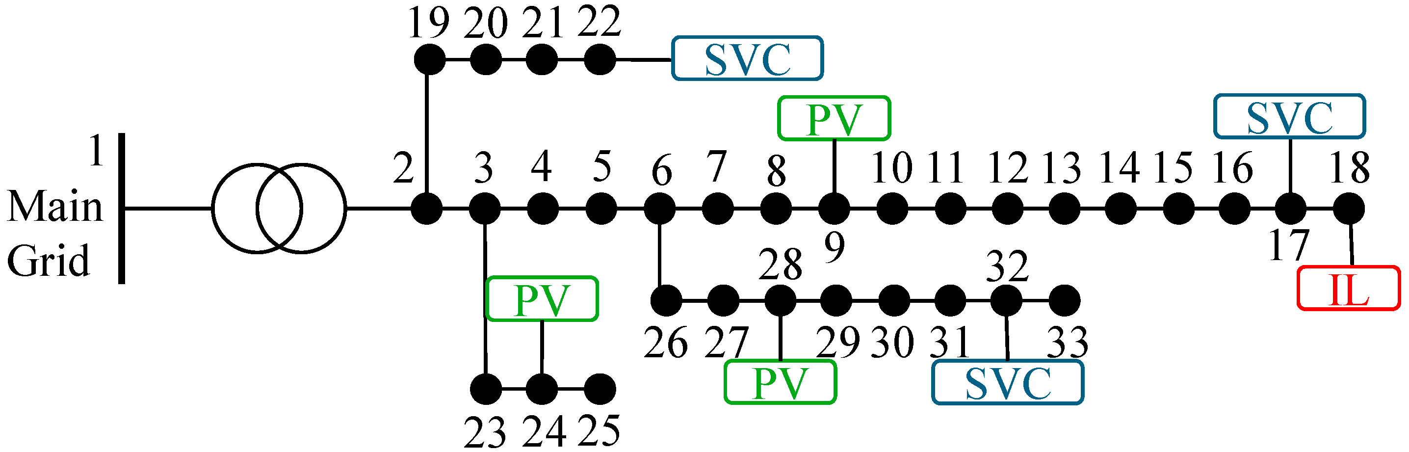
4. Case Study

This subsection is dedicated to outlining the architecture and training mechanisms of the GANs utilized in the model. These networks play a crucial role in generating synthetic but realistic scenarios of solar energy availability, which are integral to robust optimization processes. GANs consist of two main components, a generator (G) and a discriminator (D), which work in tandem through adversarial training to produce high-quality data simulations that can significantly enhance the predictive robustness of the system.

The case study is based on the IEEE 33-bus test system, with the integration of SVCs, PV units, and an IL at specific nodes, as shown in Figure 1. SVC units are installed at buses 17, 22, and 32, each with a capacity of 600 kVar, to provide reactive power compensation and support voltage regulation across the grid. PV units are connected to buses 9, 24, and 32, each with a capacity of 300 kW, contributing distributed renewable generation to the system. Additionally, an IL is connected to bus 18, providing flexibility in demand management by allowing for load shedding when required to maintain system stability. The interconnection of these components ensures a coordinated operation between renewable generation, voltage control, and demand flexibility, optimizing the performance of the IEEE 33-bus system under fluctuating conditions. Further, the PV output for 24 h is also presented in Figure 2.

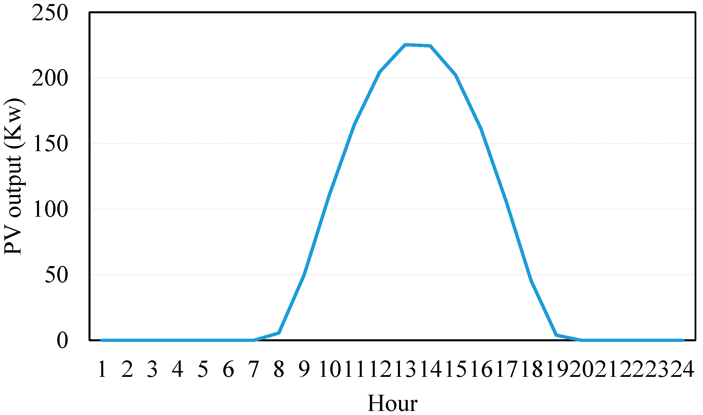
4.1. Offline Training

In this study, offline learning is conducted on a system equipped with an NVIDIA GeForce RTX 3060 GPU (manufactured by NVIDIA Corporation, headquartered in Santa Clara, CA, USA) and 16 GB of RAM. The detailed parameters of the proposed algorithm used during offline learning are provided in

Table 1. Detailed parameters of the proposed algorithm.

Parameter	Value
Structure of actor network	72 × 512 × 128 × 1
Structure of critic network	79 × 512×128 × 1
Structure of constraint network	79 × 512 × 128 × 1
Actor learning rate	1 × 10−4
Critic learning rate	1× 10−5
Optimizer	Adam
Size of minibatch	128
Entropy weight	0.12

.

Figure 3 presents the comparison of rewards obtained during offline training for three different algorithms: SAC, SAC with penalty, and the proposed method. As shown in Figure 3, the proposed method consistently outperforms both SAC and SAC with penalty in terms of overall reward. Although all methods demonstrate variability in their learning processes, the proposed method exhibits better performance, converging more quickly and with greater stability compared to the other approaches.

Figure 4 shows the comparison of constraint violation among SAC, SAC with penalty, and the proposed method, with the black dashed line representing the constraint threshold. The black dashed line in Figure 3 represents the constraint threshold or security boundary, which defines the acceptable limit for constraint violations during the training process. It serves as a benchmark to evaluate the performance of different methods in keeping costs or constraint violations below this predefined threshold. Throughout the training process, both SAC and SAC with penalty frequently exceed the threshold, indicating insufficient handling of constraints. SAC exhibits the highest level of violations, with significant fluctuations, demonstrating its inability to manage constraints effectively. While SAC with penalty offers some improvements, it still fails to consistently maintain costs below the threshold, reflecting the limitations of a simple penalty approach. In contrast, the proposed method keeps constraint violation costs consistently below the threshold, demonstrating superior performance in enforcing constraints. This highlights the proposed method’s effectiveness in balancing performance optimization with strict adherence to safety constraints, ensuring that the system operates within acceptable limits throughout the training process.

4.2. Test Results

Using the results for tests conducted over a selected day, we compared the voltage profiles of the IEEE 33-bus system under three different algorithms: SAC, SAC with penalty, and the proposed method. As shown in Figure 5a, the SAC algorithm results in several buses experiencing voltage drops below the critical threshold of 0.95 p.u., indicating significant voltage constraint violations. Figure 5b illustrates the performance of SAC with penalty, where some improvement is observed, but voltage violations still occur at certain buses, demonstrating the limited effectiveness of the penalty approach in fully ensuring constraint satisfaction. In contrast, Figure 5c shows that the proposed method keeps the voltage levels at all buses above the threshold, effectively avoiding any violations. This highlights the superior performance of the proposed method in terms of voltage regulation and constraint adherence, ensuring more reliable and stable operation of the multi-energy microgrid system compared to the other two approaches.

Table 2. Comparison of voltage regulation methods.

Method	Number of Voltage Violations	Standard Deviation of Voltage (p.u.)
SAC	2	0.0305
SAC with penalty	2	0.0023
The proposed method	0	0

compares the performance of SAC, SAC with penalty, and the proposed method in voltage regulation. It highlights that the proposed method eliminates all voltage violations and achieves the lowest standard deviation, demonstrating superior stability and adherence to voltage constraints compared to the other methods.

5. Conclusions

This paper proposes a novel VVC framework using a safe deep reinforcement learning algorithm to address real-time fluctuations in distribution networks with a high penetration of renewable energy. By formulating the VVC problem as a CMDP and incorporating a Lagrange multiplier update mechanism, the proposed method ensures that control actions adhere to safety constraints. Simulations with the IEEE 33-bus test feeder demonstrate that the SDRL-based approach significantly improves voltage regulation and reduces power losses compared to traditional methods, providing a reliable and adaptive solution for modern grid operations.

Future work could explore the integration of risk-aware reinforcement learning to enhance the proposed VVC framework, enabling more robust handling of uncertainties in renewable energy generation and dynamic load behaviors while ensuring safety and reliability in real-time grid operations.

References

1. de Mello, A.P.C.; Pfitscher, L.L.; Bernardon, D.P. Coordinated Volt/VAr control for real-time operation of smart distribution grids. Electr. Power Syst. Res. 2017, 151, 233–242. [Google Scholar] [CrossRef]
2. Zhang, Z.; Hui, H.; Song, Y. Response Capacity Allocation of Air Conditioners for Peak-Valley Regulation Considering Interaction with Surrounding Microclimate. IEEE Trans. Smart Grid 2024. [Google Scholar] [CrossRef]
3. Jia, X.; Dong, X.; Xu, B.; Qi, F.; Liu, Z.; Ma, Y.; Wang, Y. Static Voltage Stability Assessment Considering Impacts of Ambient Conditions on Overhead Transmission Lines. IEEE Trans. Ind. Appl. 2022, 58, 6981–6989. [Google Scholar] [CrossRef]
4. Niknam, T.; Zare, M.; Aghaei, J. Scenario-based multiobjective volt/var control in distribution networks including renewable energy sources. IEEE Trans. Power Deliv. 2012, 27, 2004–2019. [Google Scholar] [CrossRef]
5. Li, W.; Zou, Y.; Yang, H.; Fu, X.; Xiang, S.; Li, Z. Two stage stochastic Energy scheduling for multi energy rural microgrids with irrigation systems and biomass fermentation. IEEE Trans. Smart Grid 2024. [Google Scholar] [CrossRef]
6. Zhang, S.; Chen, S.; Gu, W.; Lu, S.; Chung, C.Y. Dynamic optimal energy flow of integrated electricity and gas systems in continuous space. Appl. Energy 2024, 375, 124052. [Google Scholar] [CrossRef]
7. Samimi, A.; Kazemi, A. Coordinated Volt/Var control in distribution systems with distributed generations based on joint active and reactive powers dispatch. Appl. Sci. 2016, 6, 4. [Google Scholar] [CrossRef]
8. Satsangi, S.; Kumbhar, G.B. Effect of load models on scheduling of VVC devices in a distribution network. IET Gener. Transm. Distrib. 2018, 12, 3993–4001. [Google Scholar] [CrossRef]
9. Li, Z.; Wu, L.; Xu, Y. Risk-Averse Coordinated Operation of a Multi-Energy Microgrid Considering Voltage/Var Control and Thermal Flow: An Adaptive Stochastic Approach. IEEE Trans. Smart Grid 2021, 12, 3914–3927. [Google Scholar] [CrossRef]
10. Gholami, K.; Azizivahed, A.; Arefi, A.; Li, L. Risk-averse Volt-VAr management scheme to coordinate distributed energy resources with demand response program. Int. J. Electr. Power Energy Syst. 2023, 146, 108761. [Google Scholar] [CrossRef]
11. Li, P.; Ji, H.; Wang, C.; Zhao, J.; Song, G.; Ding, F.; Wu, J. Coordinated Control Method of Voltage and Reactive Power for Active Distribution Networks Based on Soft Open Point. IEEE Trans. Sustain. Energy 2017, 8, 1430–1442. [Google Scholar] [CrossRef]
12. Feng, C.; Shao, L.; Wang, J.; Zhang, Y.; Wen, F. Short-term Load Forecasting of Distribution Transformer Supply Zones Based on Federated Model-Agnostic Meta Learning. IEEE Trans. Power Syst. 2024. [Google Scholar] [CrossRef]
13. Huang, H.; Li, Z.; Sampath, L.P.M.I.; Yang, J.; Nguyen, H.D.; Gooi, H.B.; Liang, R.; Gong, D. Blockchain-enabled carbon and energy trading for network-constrained coal mines with uncertainties. IEEE Trans. Sustain. Energy 2023, 14, 1634–1647. [Google Scholar] [CrossRef]
14. Xia, Y.; Xu, Y.; Feng, X. Hierarchical Coordination of Networked-Microgrids Toward Decentralized Operation: A Safe Deep Reinforcement Learning Method. IEEE Trans. Sustain. Energy 2024, 15, 1981–1993. [Google Scholar] [CrossRef]
15. Xia, Y.; Xu, Y.; Wang, Y.; Yao, W.; Mondal, S.; Dasgupta, S.; Gupta, A.K.; Gupta, G.M. A Data-Driven Method for Online Gain Scheduling of Distributed Secondary Controller in Time-Delayed Microgrids. IEEE Trans. Power Syst. 2024, 39, 5036–5049. [Google Scholar] [CrossRef]
16. Li, P.; Shen, J.; Wu, Z.; Yin, M.; Dong, Y.; Han, J. Optimal real-time Voltage/Var control for distribution network: Droop-control based multi-agent deep reinforcement learning. Int. J. Electr. Power Energy Syst. 2023, 153, 109370. [Google Scholar] [CrossRef]
17. Xia, Y.; Xu, Y.; Wang, Y.; Mondal, S.; Dasgupta, S.; Gupta, A.K.; Gupta, G.M. A Safe Policy Learning-Based Method for Decentralized and Economic Frequency Control in Isolated Networked-Microgrid Systems. IEEE Trans. Sustain. Energy 2022, 13, 1982–1993. [Google Scholar] [CrossRef]
18. Wang, W.; Yu, N.; Shi, J.; Gao, Y. Volt-VAR Control in Power Distribution Systems with Deep Reinforcement Learning. In Proceedings of the 2019 IEEE International Conference on Communications, Control, and Computing Technologies for Smart Grids (SmartGridComm), Beijing, China, 21–23 October 2019; pp. 1–7. [Google Scholar]
19. Hu, D.; Peng, Y.; Yang, J.; Deng, Q.; Cai, T. Deep Reinforcement Learning Based Coordinated Voltage Control in Smart Distribution Network. In Proceedings of the 2021 International Conference on Power System Technology (POWERCON), Haikou, China, 8–9 December 2021; pp. 1030–1034. [Google Scholar]
20. Hossain, R.; Gautam, M.; Thapa, J.; Livani, H.; Benidris, M. Deep reinforcement learning assisted co-optimization of Volt-VAR grid service in distribution networks. Sustain. Energy Grids Netw. 2023, 35, 101086. [Google Scholar] [CrossRef]
21. Gao, Y.; Yu, N. Model-augmented safe reinforcement learning for Volt-VAR control in power distribution networks. Appl. Energy 2022, 313, 118762. [Google Scholar] [CrossRef]
22. Zhang, Y.; Wang, P.; Yu, L.; Li, N.; Qiu, J. Decoupled Volt/var Control with Safe Reinforcement Learning based on Approximate Bayesian Inference. IEEE Trans. Sustain. Energy 2024. [Google Scholar] [CrossRef]
23. Liu, D.; Zeng, P.; Cui, S.; Song, C. Deep reinforcement learning for charging scheduling of electric vehicles considering distribution network voltage stability. Sensors 2023, 23, 1618. [Google Scholar] [CrossRef] [PubMed]
Figure 1. IEEE 33-bus test feeder.
Energies 18 00333 g001
Figure 2. PV output.
Energies 18 00333 g002
Figure 3. Reward comparison under different methods during offline training.
Energies 18 00333 g003
Figure 4. Cost comparison for different methods during offline training.
Energies 18 00333 g004
Figure 5. Bus voltage comparison for different methods.
Energies 18 00333 g005aEnergies 18 00333 g005b