Article

Performance Evaluation of Similarity Metrics in Transfer Learning for Building Heating Load Forecasting

1
School of Environmental Science and Engineering, Tianjin University, Tianjin 300072, China
2
School of Energy and Safety Engineering, Tianjin Chengjian University, Tianjin 300192, China
*
Author to whom correspondence should be addressed.
Energies 2025, 18(17), 4678; https://doi.org/10.3390/en18174678
Submission received: 28 July 2025 / Revised: 21 August 2025 / Accepted: 1 September 2025 / Published: 3 September 2025

Abstract

Accurately predicting building heating and cooling loads is crucial for optimizing HVAC systems and enhancing energy efficiency. However, data-driven models often face overfitting issues due to scarce training data, a common challenge for new constructions or under data privacy constraints. Transfer learning (TL) offers a solution, but its effectiveness heavily depends on selecting an appropriate source domain through effective similarity measurement. This study systematically evaluates the performance of 20 prevalent similarity metrics in TL for building heating load forecasting to identify the most robust metrics for mitigating data scarcity. Experiments were conducted on data from 500 buildings, with seven distinct low-data target scenarios established for a single target building. The Relative Error Gap (REG) was employed to assess the efficacy of transfer learning facilitated by each metric. The results demonstrate that distance-based metrics, particularly Euclidean, normalized Euclidean, and Manhattan distances, consistently yielded lower REG values and higher stability across scenarios. In contrast, probabilistic measures such as the Bhattacharyya coefficient and Bray–Curtis similarity exhibited poorer and less stable performance. This research provides a validated guideline for selecting similarity metrics in TL applications for building energy forecasting.

1. Introduction

Enhancing the efficiency of building heating and air conditioning systems is a core strategy in building energy conservation [1]. To optimize these systems, it is essential to accurately predict the cooling and heating demands of buildings, which is crucial for guiding system optimization. Therefore, accurately predicting the heating demands of buildings has become an urgent challenge to address. Currently, methods for predicting building heating demands can be broadly divided into white-box models based on physical principles and black-box models based on data [2]. White-box models, such as EnergyPlus and DeST software, rely on comprehensive building data for calculations, but such data is often difficult to fully obtain [3]. However, with the advancement of big data technology, the accumulation of building operation data is increasing, providing strong support for the development of data-driven models [4].
Starting from basic models such as support vector machines and decision trees, data-driven models have evolved to include deep learning models like multilayer perceptrons (MLP), convolutional neural networks (CNN) [5], and recurrent neural networks (RNN) [6]. These deep learning models have garnered widespread attention due to their excellent feature recognition and data adaptation capabilities, and they are often used to predict the heating and cooling loads of buildings. However, research also indicates that the performance of these models is highly dependent on the scale and quality of the data [7]. Particularly for deep learning models, a lack of training data can significantly compromise the accuracy and reliability of their predictions [8]. In practical applications, due to new construction, data protection, or cost issues, data for some buildings may be very limited, leading to severe overfitting in deep learning networks that have not been specially designed or trained with complex strategies.
When dealing with data scarcity, few-shot learning becomes a key challenge in the field of machine learning, and transfer learning is a commonly used method to address such issues [9]. Transfer learning involves learning patterns and knowledge from source tasks with abundant data and transferring them to target tasks to overcome the insufficiency of data in the target tasks [10]. Li et al. [11] employed LSTM neural networks within a pre-training and fine-tuning framework, which was shown to significantly improve the accuracy of short-term cross-building energy consumption predictions over subsequent weeks. Fan et al. [12] constructed a hybrid model combining CNN and LSTM for cross-building energy consumption forecasting, demonstrating through multiple scenarios that the approach reduces prediction errors by 15% to 78%. Santos et al. [13] developed a cross-building prediction model by integrating Transfer Learning with Temporal Fusion Transformer architectures, achieving more than a 40% reduction in prediction errors compared to non-transfer learning methods.
In the field of transfer learning, the quality of source domain data is a key factor affecting the effectiveness of transfer [14]. The excellence or inferiority of source domain data directly relates to the success of transfer learning outcomes. When there is a high similarity between the source and target domains, the pre-trained model can absorb more valuable information, thereby enhancing the transfer effect [15]. Conversely, if the similarity between the source and target domains is insufficient, the pre-trained model may struggle to capture useful knowledge, which limits the performance improvement of the target task model. In extreme cases, when the similarity between the source and target domains is very low or there are significant differences, it is not only impossible to improve the accuracy of the target task model, but it may also lead to negative transfer phenomena, reducing model performance [16]. To optimize the transfer effect, researchers have employed various metrics to assess the similarity between source and target buildings. Common methods include Maximum Information Coefficient (MIC) [17], Maximum Mean Discrepancy (MMD) [18], and Dynamic Time Warping (DTW) [19]. At the same time, scholars are exploring the potential of other algorithms in similarity assessment. For instance, Wei et al. [20] proposed a new WM algorithm to measure the similarity between source and target domains. Research results indicate that compared to algorithms like SP, PCC, MIC, JS, and WD, the WM algorithm performs better in terms of stability.
Despite numerous similarity metrics having been proposed, existing research largely focuses on comparing the performance of these metrics under a single target scenario, lacking comprehensive studies on the performance of different metrics across diverse target scenarios. Different similarity metrics are based on varying principles and are applicable to different scenarios, thus potentially exhibiting different performances in various tasks. For instance, in the field of visual recognition, Zhou et al. [21] successfully selected the optimal source domain by using KL divergence as a similarity measure. In well logging stratigraphic evaluation research, the Pearson correlation coefficient is frequently used due to its broad applicability [22]. Furthermore, when applying transfer learning methods to the problem of concrete dam deformation prediction, Chen et al. [23] achieved the best transfer effect by employing Dynamic Time Warping (DTW) as the similarity metric.
For building heating load data, which is influenced by various factors, multivariate regression models are commonly used for analysis, and the data exhibit significant time series characteristics. In the field of building heating load modeling, there is no consensus on which measurement metrics are most suitable. Therefore, this paper conducts a study aimed at evaluating data similarity metrics in the context of transfer learning for building heating load forecasting. To this end, a quantified metric—Relative Error Gap (REG)—is defined to measure the effectiveness of transfer learning, and a systematic evaluation of 20 commonly used metrics in the field of transfer learning is conducted. The study initially selects 20 commonly used metrics for measuring similarity or dissimilarity. Subsequently, 500 buildings are chosen as candidate buildings, and seven different target scenarios are set for one target building. These metrics are used for screening to implement transfer learning. Ultimately, the transfer learning results from the selected source domains are compared and analyzed with those from the optimal source domain, thereby identifying the best-performing metrics under each target scenario. This research provides valuable reference for data similarity metrics in transfer learning for building heating load forecasting.
Therefore, the primary purpose of this work is to conduct a systematic and comprehensive evaluation of 20 commonly used similarity metrics within a transfer learning framework for building heating load forecasting. We aim to identify the most effective and stable metrics under various data-scarce scenarios, thereby providing a data-driven guideline for selecting source domains and enhancing the practicality of transfer learning in real-world applications.
The innovation of this paper is the construction of an evaluation framework designed to assess similarity metrics used for screening source buildings in transfer learning methods. This framework relies on abundant building heating load data and tests the transfer performance of various metrics under different scenarios through the setting of diverse target scenarios. Furthermore, this study introduces the Relative Error Gap (REG) as a quantitative tool to measure the efficacy of metric selection and employs standard deviation to assess the stability of the transfer effects of metrics across different target scenarios, providing a comprehensive analysis of the performance of 20 similarity metrics.

2. Methodology

This section provides a detailed description of the overall research workflow. Initially, a set of similarity metrics was constructed, consisting of 20 similarity measures across six categories, to evaluate their effectiveness in transfer learning. Subsequently, seven different target scenarios were set up for a single building, and these similarity metrics were used to conduct transfer learning and test the migration effects of each metric. Finally, the REG was defined to compare the gap between the source buildings selected by each metric and the optimal source building, thereby measuring the effectiveness of their source building selection, while the standard deviation was used to assess the stability of source building selection across different scenarios. The overall process of this study is shown in Figure 1.

2.1. Constructing a Set of Similarity Metrics

In building heating load forecasting, selecting the appropriate source building is crucial for improving prediction accuracy. This process relies on various similarity metrics that can quantify the similarity between different buildings, thereby assisting in identifying the data most suitable for the target building in transfer learning. For a comprehensive evaluation, this study selected 20 commonly used similarity metrics from different fields for comparative analysis, as shown in Table 1.

2.2. Comparison of Transfer Effects in Multi-Objective Scenarios

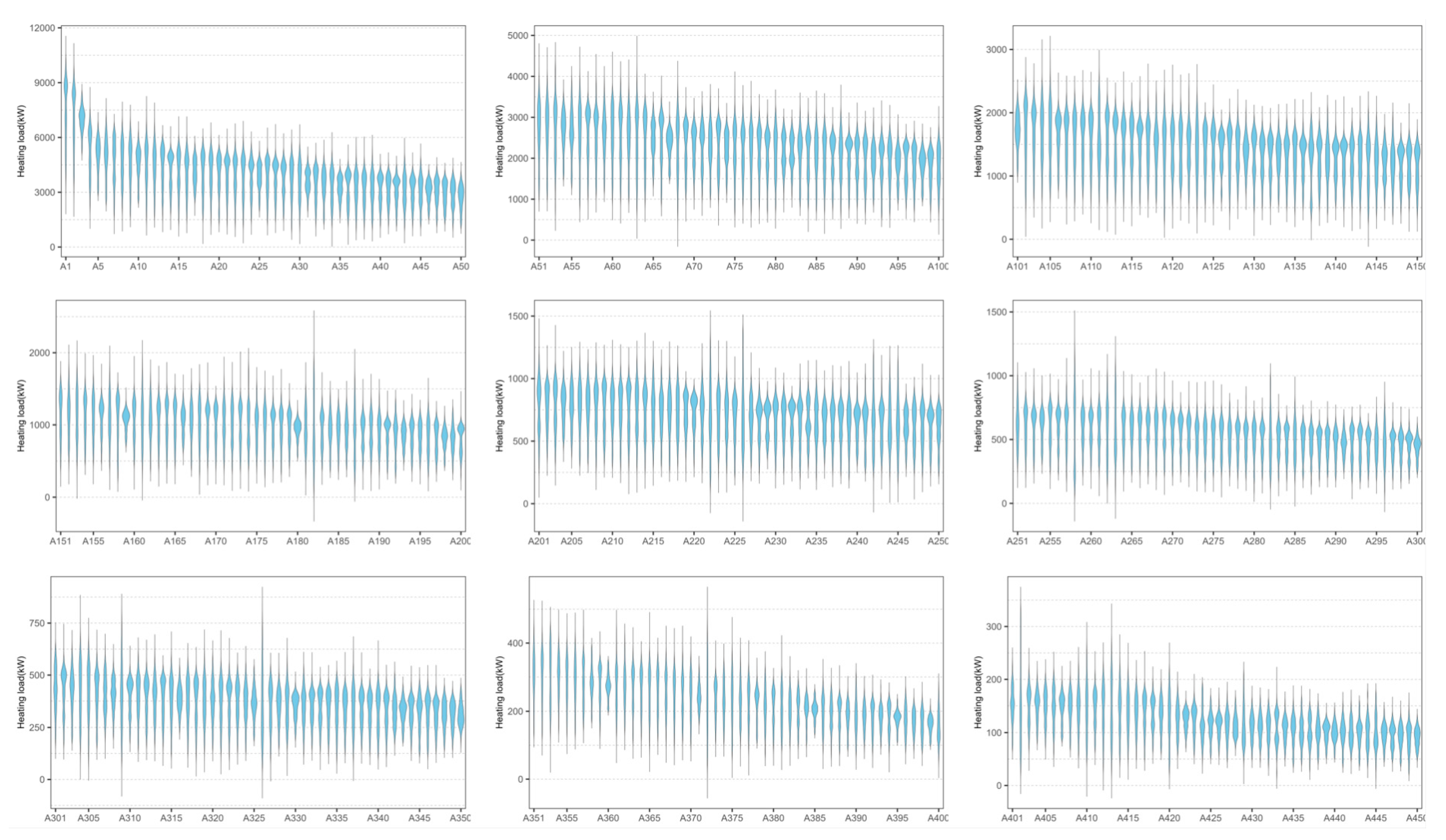
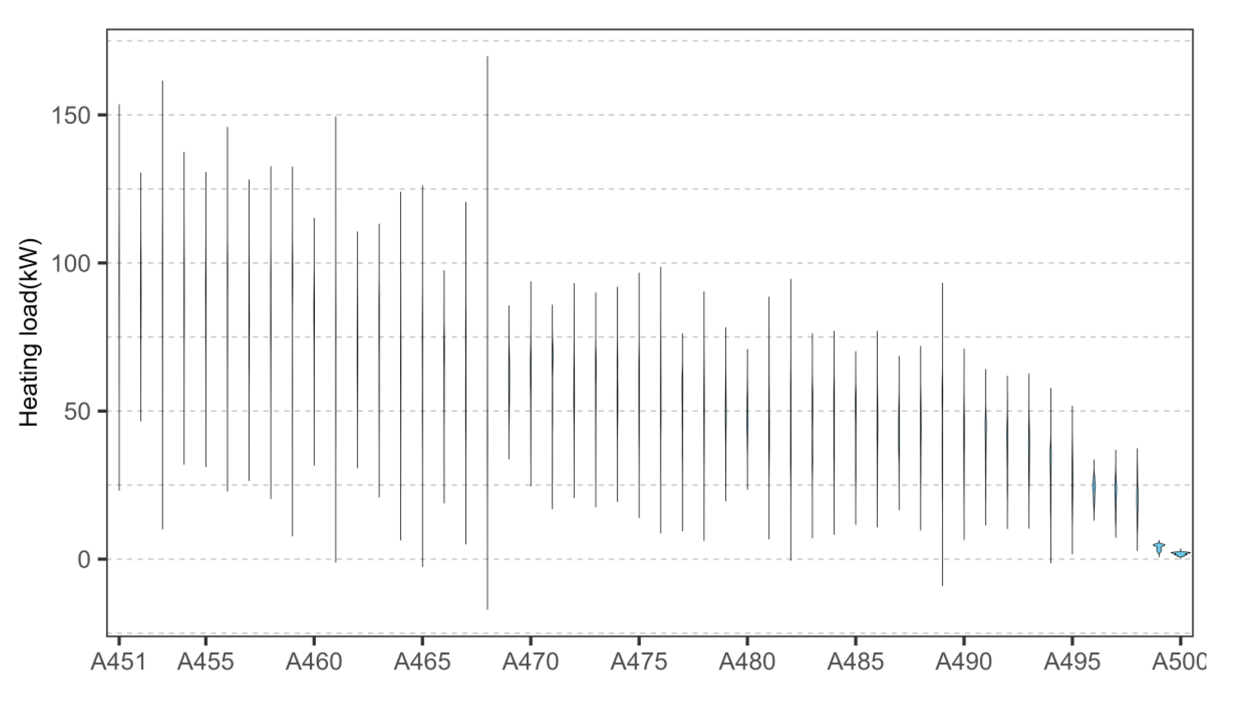
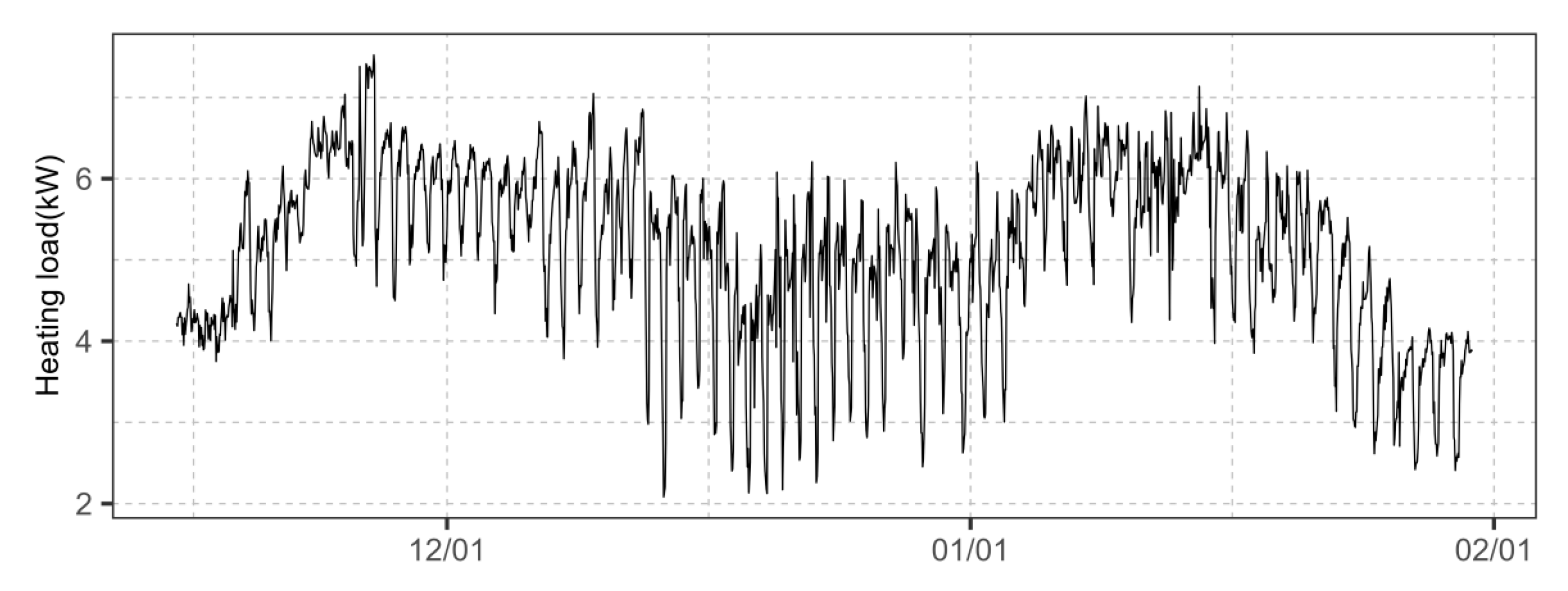
The core function of similarity metrics is to select better source buildings to enhance the accuracy of transfer learning. Specifically, the quality of the transfer effect is directly reflected in the predictive accuracy of the target task model after using these metrics to select source buildings for transfer learning. However, it is still unknown what performance indicators are suitable for measuring the similarity between building objects. The main solution of this paper is to use a large amount of building data to calculate similarity indicators and the transfer effect between buildings to analyze which indicators are suitable for task measurement in the transfer learning process. As shown in Figure 2 and Figure 3, the operating data of 500 buildings was used as the source task. Figure 4 shows the load time series data for a target building task. The data was used to set up an experiment to analyze the applicability of different indicators in the transfer learning task measurement. In addition to the hourly load data shown in Figure 2, Figure 3 and Figure 4, the data of these 501 buildings also includes data on factors affecting the load (such as outdoor temperature). Each building was monitored for hourly load and outdoor temperature data at one-hour intervals from 15 November 2024 to 1 February 2025.
As shown in Figure 1, the experimental setup is as follows: First, seven different small-sample scenarios were constructed using the target building’s data: 1 day of data available, 5 days of data available, 10 days of data available, 15 days of data available, 20 days of data available, 25 days of data available, and 30 days of data available. In each of these seven small-sample scenarios, transfer learning was performed on the target building using 500 source building task data. The last 30% of the target building data is used to test the transfer learning effect.

2.2.1. Best Source Buildings via Exhaustive Search

For each target building in the target scenarios, there theoretically exists an optimal source building among the 500 candidate buildings. The heating load data of this optimal source building, when used for transfer learning, can minimize the error of the target task model and achieve the highest prediction accuracy. The ideal goal of screening similarity is to accurately identify this best source building. Therefore, this study employs an exhaustive search method to determine the optimal source building for each target scenario and uses it as a benchmark to assess the deviation between the source buildings selected by various metrics and the optimal source building in different target scenarios. The specific steps are as follows:
Pre-train using the 500 candidate buildings to generate 500 pre-trained models.
For each target scenario, fine-tune these pre-trained models to obtain 500 target task models specific to that scenario, resulting in a total of 7 × 500 models for the 7 target scenarios.
Test the target task models for each target scenario, select the model with the smallest error as the optimal target task model, and record its corresponding source building as the optimal source building for that scenario, ultimately determining the best source buildings for 7 different scenarios.
This study employs the coefficient of variation in the root mean square error (CV-RMSE) to assess the prediction error of the target task model, as shown in Equation (1). This normalized error metric is recommended by authoritative guidelines in building performance measurement [24], as it allows for comparison across datasets with different scales.
C V R M S E = 1 μ i = 1 n x i ^ x i 2 n × 100 %
where μ represents the average actual load, x i is the actual load value, and x i ^ is the predicted load value.
It is crucial to note that this exhaustive search method is employed not as a practical tool for real-world application, but as a rigorous benchmarking technique within this research framework. While this method is computationally expensive and impractical for operational use due to the need to train and evaluate all possible models (n × m for n candidates and m scenarios), it provides an irreplaceable advantage: it guarantees the identification of the theoretically optimal source building from the candidate pool for each scenario. This establishes a definitive performance baseline (or ground truth) against which the effectiveness of all heuristic similarity metrics can be fairly and accurately measured. The computational cost was a feasible, one-time investment for this study given its fixed scope, justified by the value of obtaining an unbiased benchmark for evaluation.
The neural network model architecture used in the transfer learning process of this study is shown in Table 2, and the hyperparameter settings for the pre-training and fine-tuning processes are shown in Table 3. In this study, the input vector includes current outdoor temperature data (1 dimension), historical 12 h building heating load (12 dimensions), and historical 12 h outdoor temperature data (12 dimensions), totaling 25 dimensions. Additionally, this study assumes that the weather forecast data is sufficiently accurate, and therefore does not consider the potential impact of the uncertainty in weather forecast data on the prediction results.

2.2.2. Source Building Selection Using Similarity Metrics

After determining the optimal source building and its transfer learning effects for each target scenario, the next step is to apply similarity metrics for screening and perform transfer learning to verify the transfer effects of each metric, comparing them with the effects of the optimal source building. The specific operational steps are as follows:
In each target scenario, use each similarity metric to select what it considers the “best” source building, choosing 20 buildings per scenario, for a total of 7 × 20 source buildings.
Pre-train using these selected source buildings to generate 20 pre-trained models per target scenario, for a total of 7 × 20 pre-trained models.
Fine-tune these pre-trained models for each target scenario to form 20 target task models specific to that scenario, for a total of 7 × 20 target task models.
Test the target task models for each target scenario to assess the transfer effects of each metric in each target scenario.
The model architecture and hyperparameter settings used in these processes are the same as those in the exhaustive method, and will not be repeated here.

2.3. Evaluation of Similarity Metric Transfer Effects

The evaluation of similarity metric performance in this study is primarily conducted from two aspects: the effectiveness of the metric in selecting the best building in a single scenario and the stability of the metric’s migration effects across different scenarios. Therefore, the following two parameters are used as evaluation indicators.

2.3.1. Effectiveness Evaluation: Relative Error Gap (REG)

The role of the metric is to select a source building similar to the target building from all candidate buildings, thereby reducing the error of the target task model. Therefore, an ideal metric should be able to identify the optimal source building to minimize the error of the target task model. Therefore, to quantitatively assess the effectiveness of each similarity metric in source building selection, a normalized performance indicator is essential. The Relative Error Gap (REG) was selected for this purpose, as it provides a clear, scale-independent measure of how much worse a model performs compared to the best possible case (the benchmark). This allows for a direct and fair comparison across different target scenarios, which may have different baseline error levels. The REG is calculated as shown in Equation (2). A lower REG value indicates that the metric’s selection is closer to the optimal choice, with an REG of 0% representing a perfect selection.
R E G = ( C V R M S E ) ( C V R M S E ) m i n ( C V R M S E ) m i n

2.3.2. Stability Evaluation: Standard Deviation (SD)

The stability of a metric refers to the variation in the metric’s performance across different sample scenarios. The smaller the variation, the more consistent the metric’s performance is across different scenarios, indicating a more stable metric. Therefore, this study uses the standard deviation of the REG across different sample scenarios for each metric to assess the stability of the metric, as shown in Equation (3).
S D = n = 1 N ( R E G n R E G ¯ ) 2 N

3. Results

This section analyzes the results from Section 2, categorizing the metrics based on their performance in different scenarios, followed by a comparative analysis of the performance of different categories of metrics to identify the best-performing metrics in each scenario.

3.1. Transfer Results of Different Similarity Metrics in Different Target Scenarios

Figure 5 presents a comparison between the transfer results of all candidate buildings and those selected by each metric in different scenarios. The results indicate significant differences in the transfer effects among different source buildings. In each target scenario, the best-performing source building can reduce the model error to below 10%, while the poorest-performing source building may lead to model errors as high as 20% to 30%. Therefore, it is crucial to carefully select the source building; otherwise, arbitrary selection may result in transfer effects that fail to meet expectations. After similarity measurement, in most cases, the errors of transfer learning are maintained between 10% and 15%, which largely ensures the effectiveness of transfer learning.
However, even after similarity measurement, there are significant differences in transfer results among different metrics. Figure 6 details the transfer results of each metric in every target scenario. It can be observed that in each target scenario, there is at least a 10% gap between the best-performing and the worst-performing metrics. Therefore, it is essential to evaluate which metrics can minimize the error of the target task model to the greatest extent in each target scenario, to prevent improper metric selection from affecting the transfer effects.

3.2. Classification of Metrics Based on Source Domain Selection Results

Table 4 details the source domain selection results for each metric across various target scenarios. For easy identification, metrics with the same source domain are marked with the same background color. Based on these selection results, all 20 metrics can be categorized into 6 different groups. It is noteworthy that metrics within the same group show consistency in their source domain selection across various target scenarios. The categorization of the 20 metrics into the 6 distinct groups presented in Table 4 was not arbitrary but was driven by the empirical results of the source domain selection process. The grouping was performed based on a clear and objective principle: metrics that consistently selected the identical source building across all seven target scenarios were clustered into the same group.
According to the classification results, it can be observed that the metrics in Group 1 exhibit a high degree of consistency, which may imply that they are more reliable in transfer learning. In contrast, the metrics in Groups 2 to 6 show more variation in their selections across different target scenarios, indicating that finer adjustments may be needed based on specific contexts in practical applications. Additionally, it can be observed that as the time dimension of the target scenarios increases, the source domain selection for certain metrics (such as Cosine Similarity in Group 3) changes. This may suggest that the distribution characteristics of the data may evolve over time, thereby affecting the choice of metrics.

3.3. REG of Each Group’s Transfer Effects Compared to the Best Transfer Effects

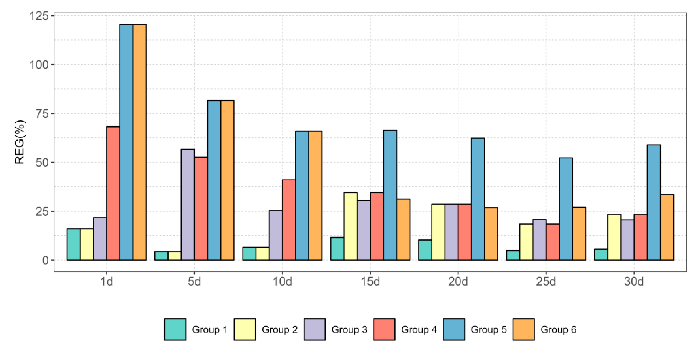
Figure 7 illustrates the REG values for each category of metrics (Group 1 to Group 6) across different target scenarios. The REG value is a key indicator for measuring the effectiveness of transfer learning, calculated based on the relative error gap between the pre-trained model and the optimal pre-trained model.
The REG results, detailed in Figure 7, reveal a clear hierarchy in metric performance. Metrics in Group 1 (Euclidean, Manhattan, KL Divergence, etc.) consistently achieved the lowest REG values across nearly all target scenarios. This superior performance can be attributed to the nature of building heating load data and the mathematical principles of these metrics. As analyzed in Section 2.1, these are primarily distance-based and distribution-based metrics. They excel at quantifying the absolute geometric proximity or probability distribution discrepancy between multi-dimensional feature vectors (e.g., outdoor temperature, historical loads). This aligns perfectly with the regression task of load forecasting, where the model must learn a mapping from input features to a continuous output value. A source building with minimal distance or distributional divergence is likely to provide a pre-trained model whose internal representations are already well-suited for the target task, requiring only minor fine-tuning adjustments.
Notably, the metrics in Group 2 (Chebyshev) performed on par with Group 1 in ultra-short-term scenarios (1d to 10d) but exhibited a noticeable performance decline as more data became available. This suggests that the Chebyshev distance (which focuses on the maximum difference in any single dimension) is sensitive to noise or outliers in very small datasets but becomes a less comprehensive measure of overall similarity as the data volume increases and the feature relationships become more complex.
Conversely, the metrics in Groups 4 to 6 (e.g., Bhattacharyya, Bray–Curtis, Pearson) consistently yielded higher REG values, indicating poorer performance. This finding provides a crucial confirmation of our hypothesis: not all similarity measures are equally effective. For instance, correlation-based metrics like Pearson (Group 6) focus solely on the linear trend between sequences but are invariant to scale. This means they might select a source building whose load profile has a similar shape but a vastly different magnitude, leading to a poor initialization for the fine-tuning process. Similarly, Bhattacharyya and Bray–Curtis (Group 4), often used for measuring distribution overlap in categorical or compositional data, appear less suited to capturing the geometric distances critical in this high-dimensional, real-valued regression problem.
The instability of Cosine Similarity (Group 3), as seen by its fluctuating REG and high standard deviation, further underscores the importance of magnitude in this context. While it measures the angle between vectors, ignoring their length, it can be misled by profiles that are directionally similar but energetically dissimilar.
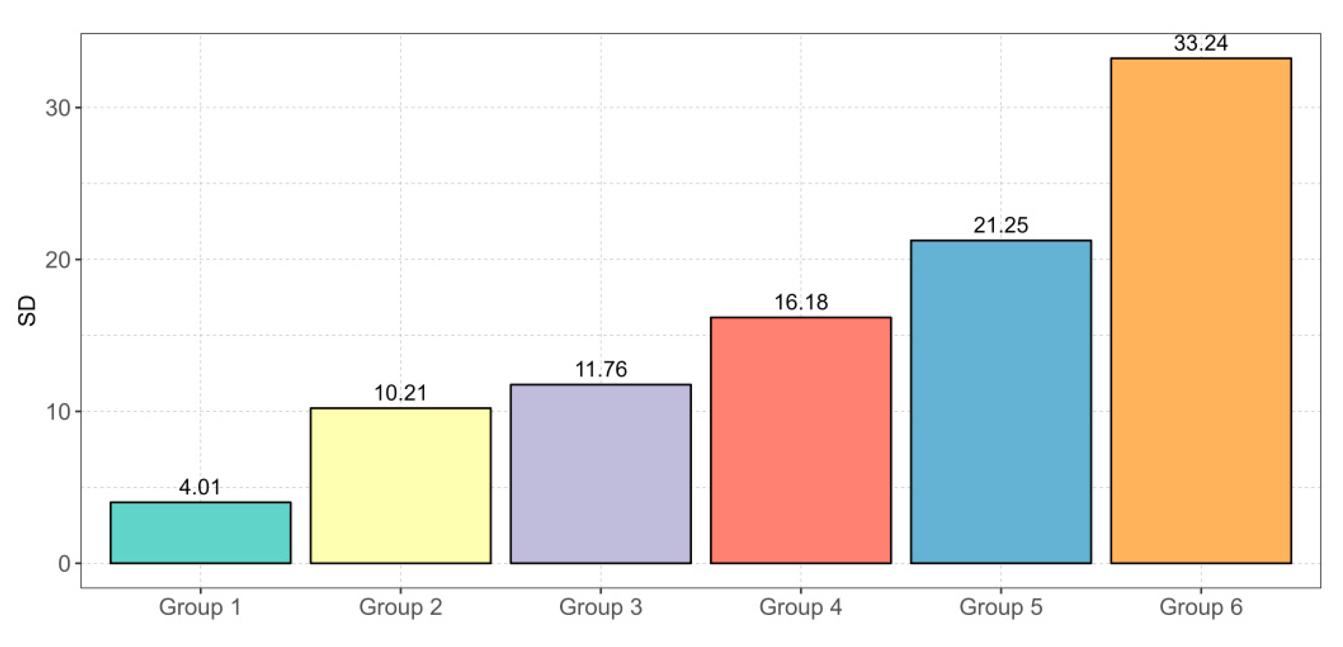
Figure 8 analyzes the standard deviation of the REG values for each type of metric, revealing the stability of metric performance across different target scenarios. Metrics in Group 1 not only perform excellently in terms of REG values but also maintain a low standard deviation, demonstrating superior stability. This implies that these metrics can maintain their high performance in a variety of target scenarios. In contrast, metrics in Groups 2 and 3, while having decent REG values in some scenarios, exhibit a larger standard deviation, suggesting that their performance may fluctuate significantly across different scenarios. This could be related to their sensitivity to data characteristics or the variability in the source buildings they select. The metrics in Groups 4 to 6, however, not only have higher REG values but also a larger standard deviation, indicating that their performance in the transfer learning process is not only poor but also unstable. This may suggest that they are not suitable for building heating load forecasting problems.
The superior and stable performance of Group 1 metrics (e.g., Euclidean, Manhattan, KL Divergence) can be attributed to the nature of building heating load data and the fundamental principles of these metrics. Heating load time series are typically characterized by multi-dimensional, real-valued data points (e.g., temperature, historical loads) where the absolute magnitude and overall distribution similarity are crucial for effective knowledge transfer.
Group 1 metrics are predominantly distance-based (Euclidean, Manhattan) or distribution-based (KL, JS, Hellinger). These metrics are highly effective at quantifying the overall geometric proximity or probability distribution discrepancy between the source and target building’s feature vectors. This aligns well with the regression task of load forecasting, where the model must learn to map input features to a continuous load value. A source building with minimal geometric or distributional distance in its feature space is likely to provide a pre-trained model whose feature representations are already well-suited for the target task, requiring only minor fine-tuning.
In contrast, metrics that underperformed, such as the Bhattacharyya coefficient or Bray–Curtis similarity (Group 4), are often more suited for measuring overlap between probability distributions or compositional data rather than geometric distances in a high-dimensional feature space. Similarly, correlation-based metrics like Pearson (Group 6) focus solely on the linear trend between sequences but are invariant to scale, meaning they might select a source building whose load profile has a similar shape but a vastly different magnitude, leading to poor transfer performance. The instability of Cosine Similarity (Group 3) with increasing data length suggests that the angle between data vectors becomes a less reliable indicator than their absolute distance as the temporal context becomes richer and more complex.

4. Conclusions

This paper provides an in-depth exploration of the performance evaluation of similarity metrics in transfer learning methods for building heating load forecasting through systematic experiments and analysis. The findings reveal the effectiveness and applicability of different metrics in transfer learning strategies, offering clear guidance for building heating load forecasting issues.
  • There is a significant difference in the effectiveness of various similarity metrics in transfer learning strategies. The metrics in Group 1 (such as Euclidean distance) have low REG values (an average of 5%) in most scenarios, with transfer effects close to optimal. In contrast, metrics in Groups 4 to 6 (such as Bhattacharyya coefficient) have high REG values (an average of 15%), exhibiting poor performance and stability.
  • Stability evaluation indicators show that while metrics in Group 1 demonstrate excellent REG values, they also maintain a low standard deviation, with an average of 2%, indicating superior stability. Certain metrics in Groups 2 and 3 perform well in specific scenarios but have a larger standard deviation (an average of 5%), indicating performance fluctuations. Metrics in Groups 4 to 6 have both high REG values and standard deviations (an average of 8%), indicating poor stability.
  • As the time dimension of the target scenarios increases, the selection of source domains by certain metrics (such as Cosine Similarity in Group 3) changes. Cosine Similarity has a low REG value in the short term (an average of 6%), but as the time grows to 10 to 30 days, the REG value rises to 10%. This may indicate that as time progresses, the distribution characteristics of the data change, thereby affecting the selection of the metric.
  • The underlying reason for the superior performance of Group 1 metrics lies in their alignment with the data characteristics of the building heating load forecasting problem. Distance and distribution metrics effectively capture the geometric and statistical similarities in the multi-variate input features that are most relevant for the regression model. This suggests that for transfer learning in building energy forecasting, metrics that prioritize overall magnitude and distribution alignment are more reliable than those focused solely on trend similarity or distribution overlap.

Author Contributions

Conceptualization, H.M.; methodology, D.B.; software, D.B.; validation, D.B.; formal analysis, D.B.; investigation, D.B.; resources, S.M.; data curation, D.B.; writing—original draft preparation, D.B.; writing—review and editing, S.M.; visualization, D.B. All authors have read and agreed to the published version of the manuscript.

Funding

This research received no external funding.

Data Availability Statement

Due to confidentiality issues related to the project, the author does not have permission to disclose the data.

Conflicts of Interest

The authors declare no conflicts of interest.

References

  1. Zhu, D.; Hong, T.; Yan, D.; Wang, C. A detailed loads comparison of three building energy modeling programs: EnergyPlus, DeST and DOE-2.1 E. Build. Simul. 2013, 6, 323–335. [Google Scholar] [CrossRef]
  2. Jiao, Y.; Tan, Z.; Zhang, D.; Zheng, Q.P. Short-term building energy consumption prediction strategy based on modal decomposition and reconstruction algorithm. Energy Build. 2023, 290, 113074. [Google Scholar] [CrossRef]
  3. Tian, W.; Yang, S.; Li, Z.; Wei, S.; Pan, W.; Liu, Y. Identifying informative energy data in Bayesian calibration of building energy models. Energy Build. 2016, 119, 363–376. [Google Scholar] [CrossRef]
  4. Ali, U.; Bano, S.; Shamsi, M.H.; Sood, D.; Hoare, C.; Zuo, W.; O’Donnell, J. Urban building energy performance prediction and retrofit analysis using data-driven machine learning approach. Energy Build. 2024, 303, 113768. [Google Scholar] [CrossRef]
  5. Li, K.; Mu, Y.; Yang, F.; Wang, H.; Yan, Y.; Zhang, C. A novel short-term multi-energy load forecasting method for integrated energy system based on feature separation-fusion technology and improved CNN. Appl. Energy 2023, 351, 121823. [Google Scholar] [CrossRef]
  6. Zhou, M.; Wang, L.; Hu, F.; Zhu, Z.; Zhang, Q.; Kong, W.; Cui, E. ISSA-LSTM: A new data-driven method of heat load forecasting for building air conditioning. Energy Build. 2024, 321, 114698. [Google Scholar] [CrossRef]
  7. Lu, Y.; Peng, X.; Li, C.; Tian, Z.; Kong, X.; Niu, J. Few-sample model training assistant: A meta-learning technique for building heating load forecasting based on simulation data. Energy 2025, 317, 134509. [Google Scholar] [CrossRef]
  8. Wang, Y.; Yao, Q.; Kwok, J.T.; Ni, L.M. Generalizing from a few examples: A survey on few-shot learning. ACM Comput. Surv. 2020, 53, 1–34. [Google Scholar] [CrossRef]
  9. Genkin, M.; McArthur, J.J. A transfer learning approach to minimize reinforcement learning risks in energy optimization for automated and smart buildings. Energy Build. 2024, 303, 113760. [Google Scholar] [CrossRef]
  10. Obayya, M.; Alotaibi, S.S.; Dhahb, S.; Alabdan, R.; Al Duhayyim, M.; Hamza, M.A.; Motwakel, A. Optimal deep transfer learning based ethnicity recognition on face images. Image Vis. Comput. 2022, 128, 104584. [Google Scholar] [CrossRef]
  11. Li, G.; Wu, Y.; Liu, J.; Fang, X.; Wang, Z. Performance evaluation of short-term cross-building energy predictions using deep transfer learning strategies. Energy Build. 2022, 275, 112461. [Google Scholar] [CrossRef]
  12. Fan, C.; Sun, Y.; Xiao, F.; Ma, J.; Lee, D.; Wang, J.; Tseng, Y.C. Statistical investigations of transfer learning-based methodology for short-term building energy predictions. Appl. Energy 2020, 262, 114499. [Google Scholar] [CrossRef]
  13. Santos, M.L.; García, S.D.; García-Santiago, X.; Ogando-Martínez, A.; Camarero, F.E.; Gil, G.B.; Ortega, P.C. Deep learning and transfer learning techniques applied to short-term load forecasting of data-poor buildings in local energy communities. Energy Build. 2023, 292, 113164. [Google Scholar] [CrossRef]
  14. Qian, F.; Gao, W.; Yang, Y.; Yu, D. Potential analysis of the transfer learning model in short and medium-term forecasting of building HVAC energy consumption. Energy 2020, 193, 116724. [Google Scholar] [CrossRef]
  15. Ben-David, S.; Blitzer, J.; Crammer, K.; Pereira, F. Analysis of representations for domain adaptation. In Advances in Neural Information Processing Systems; MIT Press: Cambridge, MA, USA, 2006; Volume 19. [Google Scholar]
  16. Lim, B.; Arık, S.Ö.; Loeff, N.; Pfister, T. Temporal fusion transformers for interpretable multi-horizon time series forecasting. Int. J. Forecast. 2021, 37, 1748–1764. [Google Scholar] [CrossRef]
  17. Lu, Y.; Wang, G.; Huang, S. A short-term load forecasting model based on mixup and transfer learning. Electr. Power Syst. Res. 2022, 207, 107837. [Google Scholar] [CrossRef]
  18. Yuan, Y.; Chen, Z.; Wang, Z.; Sun, Y.; Chen, Y. Attention mechanism-based transfer learning model for day-ahead energy demand forecasting of shopping mall buildings. Energy 2023, 270, 126878. [Google Scholar] [CrossRef]
  19. Xing, Z.; Pan, Y.; Yang, Y.; Yuan, X.; Liang, Y.; Huang, Z. Transfer learning integrating similarity analysis for short-term and long-term building energy consumption prediction. Appl. Energy 2024, 365, 123276. [Google Scholar] [CrossRef]
  20. Wei, N.; Yin, C.; Yin, L.; Tan, J.; Liu, J.; Wang, S.; Zeng, F. Short-term load forecasting based on WM algorithm and transfer learning model. Appl. Energy 2024, 353, 122087. [Google Scholar] [CrossRef]
  21. Zhou, H.; Luo, T.; He, Y. Dynamic collaborative learning with heterogeneous knowledge transfer for long-tailed visual recognition. Inf. Fusion 2025, 115, 102734. [Google Scholar] [CrossRef]
  22. Xu, B.; Feng, Z.; Zhou, J.; Shao, R.; Wu, H.; Liu, P.; Xiao, L. Transfer learning for well logging formation evaluation using similarity weights. Artif. Intell. Geosci. 2024, 5, 100091. [Google Scholar] [CrossRef]
  23. Chen, X.; Chen, Z.; Hu, S.; Gu, C.; Guo, J.; Qin, X. A feature decomposition-based deep transfer learning framework for concrete dam deformation prediction with observational insufficiency. Adv. Eng. Inform. 2023, 58, 102175. [Google Scholar] [CrossRef]
  24. ASHRAE. ASHRAE Guideline 14-2014: Measurement of Energy, Demand, and Water Savings; American Society of Heating, Refrigerating and Air-Conditioning Engineers: Atlanta, GA, USA, 2014. [Google Scholar]
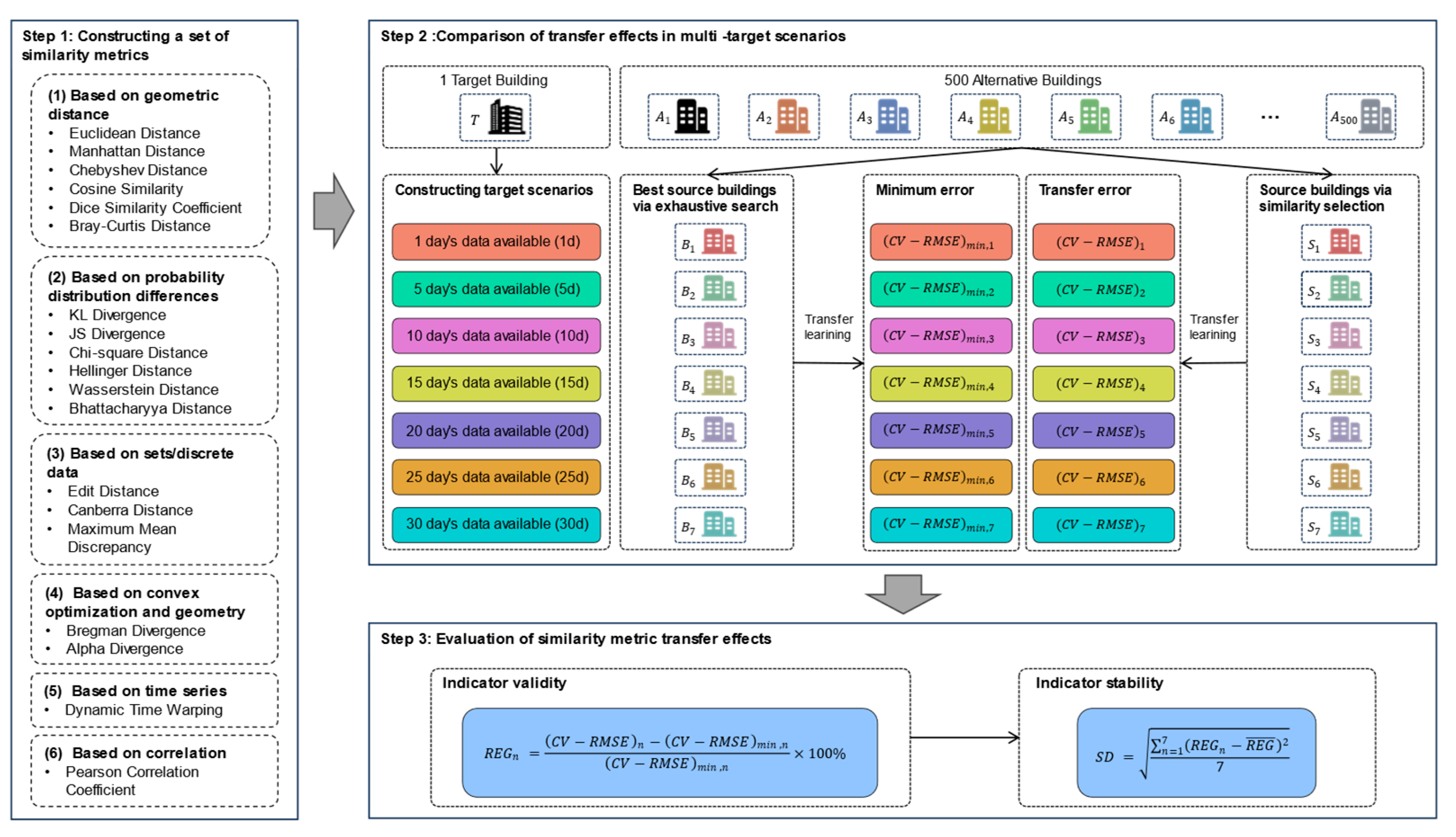
Figure 1. Overall Workflow of This Study.
Energies 18 04678 g001
Figure 2. Alternative source buildings A 1 to A 450 .
Energies 18 04678 g002
Figure 3. Alternative source buildings A 451 to A 500 .
Energies 18 04678 g003
Figure 4. The heating load time series of target building T .
Energies 18 04678 g004
Figure 5. Comparison of Transfer Results for All Candidate Buildings and Source Buildings Selected by Each Metric in Different Scenarios.
Energies 18 04678 g005
Figure 6. Transfer Results of Individual Metrics.
Energies 18 04678 g006
Figure 7. REG for Each Category of Metrics in Different Target Scenarios.
Energies 18 04678 g007
Figure 8. Standard Deviation of REG for Each Category of Metrics in Different Target Scenarios.
Energies 18 04678 g008
Table 1. The similarity metrics selected in this study.
CategoryMetricDescription
Based on geometric distanceEuclidean DistanceMeasures the straight-line distance between two points in space.
Manhattan DistanceSums the absolute differences between points along each dimension.
Chebyshev DistanceFinds the maximum difference between any two dimensions of the points.
Cosine SimilarityCompares the direction of vectors, not their magnitude.
Dice Similarity CoefficientCompares the overlap between two sets.
Bray–Curtis DistanceMeasures similarity based on the ratio of shared to total items.
Based on probability distribution differencesKL DivergenceCompares how one probability distribution diverges from a second, expected distribution.
JS DivergenceA symmetric version of KL Divergence, measuring the average difference between two distributions.
Chi-square DistanceCompares observed and expected frequencies in categorical data.
Hellinger DistanceMeasures the similarity between two probability distributions.
Wasserstein DistanceMeasures the distance between probability distributions.
Bhattacharyya DistanceCompares the overlap between two probability distributions.
Based on sets/discrete dataEdit DistanceCalculates the minimum number of operations to transform one string into another.
Canberra DistanceCompares the ratio of differences in corresponding elements of two vectors.
Maximum Mean Discrepancy (MMD)Compares the difference between the means of two distributions.
Based on convex optimization and geometryBregman DivergenceMeasures the difference between two points using a convex function.
Alpha DivergenceA flexible measure of the difference between probability distributions.
Based on time seriesDynamic Time Warping (DTW)Aligns and compares time series data, accounting for time shifts.
Based on correlationPearson Correlation CoefficientMeasures the linear relationship between two variables.
Table 2. Neural Network Architecture Used in This Study.
LayerNumber of NeuronsActivation Function
Input25-
Hidden Layer 1100ReLU
Dropout--
Hidden Layer 2100ReLU
Dropout--
Hidden Layer 3100ReLU
Dropout--
Output1Linear
Table 3. Hyperparameter Settings for Transfer Learning in This Study.
BatchEpochsLearning Rate
Pre-training323000.001
Fine-tuning32100.0001
Table 4. Source Domain Selection Results for Each Metric in Different Target Scenarios.
1d5d10d15d20d25d30d
Group 1EuclideanA237A237A237A237A237A237A237
Standardized EuclideanA237A237A237A237A237A237A237
ManhattanA237A237A237A237A237A237A237
Chi-squareA237A237A237A237A237A237A237
KL DivergenceA237A237A237A237A237A237A237
JS DivergenceA237A237A237A237A237A237A237
HellingerA237A237A237A237A237A237A237
Alpha DivergenceA237A237A237A237A237A237A237
Bregman DivergenceA237A237A237A237A237A237A237
MMDA237A237A237A237A237A237A237
DiceA237A237A237A237A237A237A237
Group 2ChebyshevA237A237A237A89A89A89A89
Group 3CosineA415A302A176A176A176A176A176
Group 4BhattacharyyaA89A89A89A89A89A89A89
Bray–CurtisA89A89A89A89A89A89A89
DTWA89A89A89A89A89A89A89
Wasserstein DistanceA89A89A89A89A89A89A89
Group 5CanberraA421A421A421A421A421A421A421
EditA421A421A421A421A421A421A421
Group 6PearsonA421A421A421A58A58A311A311
Disclaimer/Publisher’s Note: The statements, opinions and data contained in all publications are solely those of the individual author(s) and contributor(s) and not of MDPI and/or the editor(s). MDPI and/or the editor(s) disclaim responsibility for any injury to people or property resulting from any ideas, methods, instructions or products referred to in the content.