Article

Machine Learning Approaches for Predicting Lithological and Petrophysical Parameters in Hydrocarbon Exploration: A Case Study from the Carpathian Foredeep

by
Drozd Arkadiusz
*,
Topór Tomasz
,
Lis-Śledziona Anita
and
Sowiżdżał Krzysztof
Oil and Gas Institute—National Research Institute, Lubicz Street 25A, 31-503 Krakow, Poland
*
Author to whom correspondence should be addressed.
Energies 2025, 18(17), 4521; https://doi.org/10.3390/en18174521
Submission received: 17 June 2025 / Revised: 30 July 2025 / Accepted: 14 August 2025 / Published: 26 August 2025
(This article belongs to the Section H1: Petroleum Engineering)

Abstract

This study presents a novel approach to the parametrization of 3D PETRO FACIES and SEISMO FACIES using supervised and unsupervised learning, supported by a coherent structural and stratigraphic framework, to enhance understanding of the presence of hydrocarbons in the Dzików–Uszkowce region. The prediction relies on selected seismic attributes and well logging data, which are essential in hydrocarbon exploration. Three-dimensional seismic data, a crucial source of information, reflect the propagation velocity of elastic waves influenced by lithological formations and reservoir fluids. However, seismic response similarities complicate accurate seismic image interpretation. Three-dimensional seismic data were also used to build a structural–stratigraphic model that partitions the study area into coeval strata, enabling spatial analysis of the machine learning results. In the 3D seismic model, PETRO FACIES classification achieved an overall accuracy of 80% (SD = 0.01), effectively distinguishing sandstone- and mudstone-dominated facies (RT1–RT4) with F1 scores between 0.65 and 0.85. RESERVOIR FACIES prediction, covering seven hydrocarbon system classes, reached an accuracy of 70% (SD = 0.01). However, class-level performance varied substantially. Non-productive zones such as HNF (No Flow) were identified with high precision (0.82) and recall (0.84, F1 = 0.83), while mixed-saturation facies (HWGS, BSWGS) showed moderate performance (F1 = 0.74–0.81). In contrast, gas-saturated classes (BSGS and HGS) suffered from extremely low F1 scores (0.08 and 0.12, respectively), with recalls as low as 5–7%, highlighting the model’s difficulty in discriminating these units from water-saturated or mixed facies due to overlapping seismic responses and limited training data for gas-rich intervals. To enhance reservoir characterization, SEISMO FACIES analysis identified 12 distinct seismic facies using key attributes. An additional facies (facies 13) was defined to characterize gas-saturated sandstones with high reservoir quality and accumulation potential. Refinements were performed using borehole data on hydrocarbon-bearing zones and clay volume (VCL), applying a 0.3 VCL cutoff and filtering specific facies to isolate zones with confirmed gas presence. The same approach was applied to PETRO FACIES and a new RT facie was extracted. This integrated approach improved mapping of lithological variability and hydrocarbon saturation in complex geological settings. The results were validated against two blind wells that were excluded from the machine learning process. Knowledge of the presence of gas in well N-1 and its absence in well D-24 guided verification of the models within the structural–stratigraphic framework.

1. Introduction

The Miocene deposits of the Carpathian Foredeep are characterized by distinct lithological development, commonly forming heterolithic sandstone–mudstone successions. These deposits reflect deposition in different sedimentological environments, where lithological variability, fine-scale bedding, and cyclic alternation of reservoir and seal layers create complex reservoir architectures [1,2]. This heterogeneity results in a variable seismic response, often complicated further by the presence of hydrocarbons, which may significantly alter acoustic properties and give rise to seismic anomalies.
Recent studies by Antariksa et al. [3], Feng [4], and Wang [5] demonstrate the growing application of both supervised and unsupervised machine learning techniques in the classification of facies, lithotypes, and SEISMO FACIES. These methods increasingly incorporate the fusion of multiple algorithms to enhance the accuracy and reliability of lithofacies prediction. For example, Wang [5] proposed a novel lithology identification approach that integrates the Hidden Markov Model with the Random Forest algorithm, effectively combining probabilistic modeling with ensemble learning to improve classification outcomes. Okpoli and Arogunyo [6] presented a case study from the onshore Niger Delta, where the integration of well log data with seismic interpretation facilitated accurate field delineation and reservoir identification. They assessed reservoir quality using key petrophysical parameters, including gamma ray, bulk density, porosity, and resistivity. Their analysis emphasized that zones of low density and high resistivity may suggest the presence of hydrocarbons, but only when supported by a coherent structural and stratigraphic framework. Furthermore, they demonstrated that advanced seismic attribute analysis—particularly the use of variance attribute mapping—enhances the detection of subtle faults and structural traps that may be overlooked in conventional seismic interpretation. A comparable methodology was employed by Pietsch and Jarzyna [7] in the Miocene deposits of the Polish Carpathian Foredeep. By integrating well log data with seismic modeling, they successfully identified potential gas-bearing intervals. Their work highlighted the importance of selecting appropriate petrophysical parameters and incorporating velocity models that account for wave attenuation. Another example of the application of these methods was provided by Łukaszewski [8]. The author analyzed 3D seismic data from the Carpathian Foredeep using the GLCM method to extract texture attributes (Energy and Entropy), enabling the identification of a submarine channel system and potential gas-bearing zones. The results demonstrated a strong correlation between attributes and reservoir presence, validating their suitability as an input for machine learning-based facies classification.
The identification and delineation of gas-bearing zones within heterolithic formations present significant challenges due to their complex lithological variability and discontinuous reservoir properties. In such settings, advanced machine learning techniques offer promising support by enhancing pattern recognition and improving the classification of subtle geophysical and petrophysical indicators.
Seismic anomalies such as bright spots and time sag effects have become valuable direct hydrocarbon indicators in Miocene formations. Their occurrence is primarily linked to the presence of gas-saturated porous sandstones, which reduce seismic wave velocity and create high-contrast reflection boundaries. However, not all anomalies are indicative of commercial gas accumulations. Similar seismic responses can arise from lithological heterogeneities or from zones saturated with water containing minor amounts of gas, which may lead to misinterpretation [9].
As a result, conventional methods of gas horizon identification often prove insufficient, especially in such fine-scale heterolithic systems. This necessitates the use of advanced sedimentological models and high-resolution geophysical techniques to reliably identify and evaluate potential gas-bearing intervals. This study introduces supervised and unsupervised learning-based approaches for 3D PETRO FACIES and SEISMO FACIES parametrization, underpinned by a robust structural and stratigraphic framework, aimed at refining predictions of hydrocarbon presence in the Dzików–Uszkowce area. The methodology described in the paper is the first of its kind to be applied in the Carpathian Foredeep region.

2. Location and Description of the Study Area

The study area is located in the northeastern part of the Carpathian Foredeep (Figure 1a), which is filled with Lower and Middle Miocene autochthonous deposits, formed under the varying sedimentary conditions of the foreland basin (Figure 1b) [10]. The Carpathian Foredeep can be divided into an external part, located north of the Carpathians, and an internal part, currently hidden beneath the overthrust Carpathians. The external part of the foredeep, where the study area is located, is filled with Middle Miocene marine deposits, with a thickness ranging from several hundred meters in the northern marginal part to approximately 3000 m in the southeastern part [11].
The Dzików and Uszkowce areas are filled with Upper Badenian and Sarmatian deposits, characterized by complex lithological and tectonic structures and high facies variability (Figure 1b). In Dzików, the Lower Sarmatian succession is developed as a sandstone–mudstone series with distinct lamination and both vertical and lateral heterogeneity. Sandstone lenses and pinch-outs within clay-rich intervals play a key role in forming gas traps. Gas accumulations are mainly located in the upper parts of these sequences. The deposits consist predominantly of gray, locally sandy mudstones interbedded with fine- to medium-grained sandstones containing mica.
Dzików sandstones form locally developed, lenticular bodies within muddy facies, typically associated with deltaic depositional systems. These sandstones exhibit good reservoir properties due to their relatively high porosity and weak cementation. Gas accumulations are commonly confined to the sandy bodies, which differ significantly in composition and structure from the more laminated and clay-rich upper Sarmatian deposits.
In Uszkowce, hydrocarbon exploration targets autochthonous Miocene sediments. The reservoir rocks comprise fine- to medium-grained, clayey gray sandstones with carbonate or carbonate-clay cement and occasional subtle lamination. The grains are poorly rounded and moderately sorted, with admixtures of glauconite, mica, and plant debris. These are accompanied by darker siltstones and claystones rich in organic matter, acting as effective seals. The sealing units are calcareous, marly clays with wavy lamination and uneven fracture surfaces.

3. Methodology

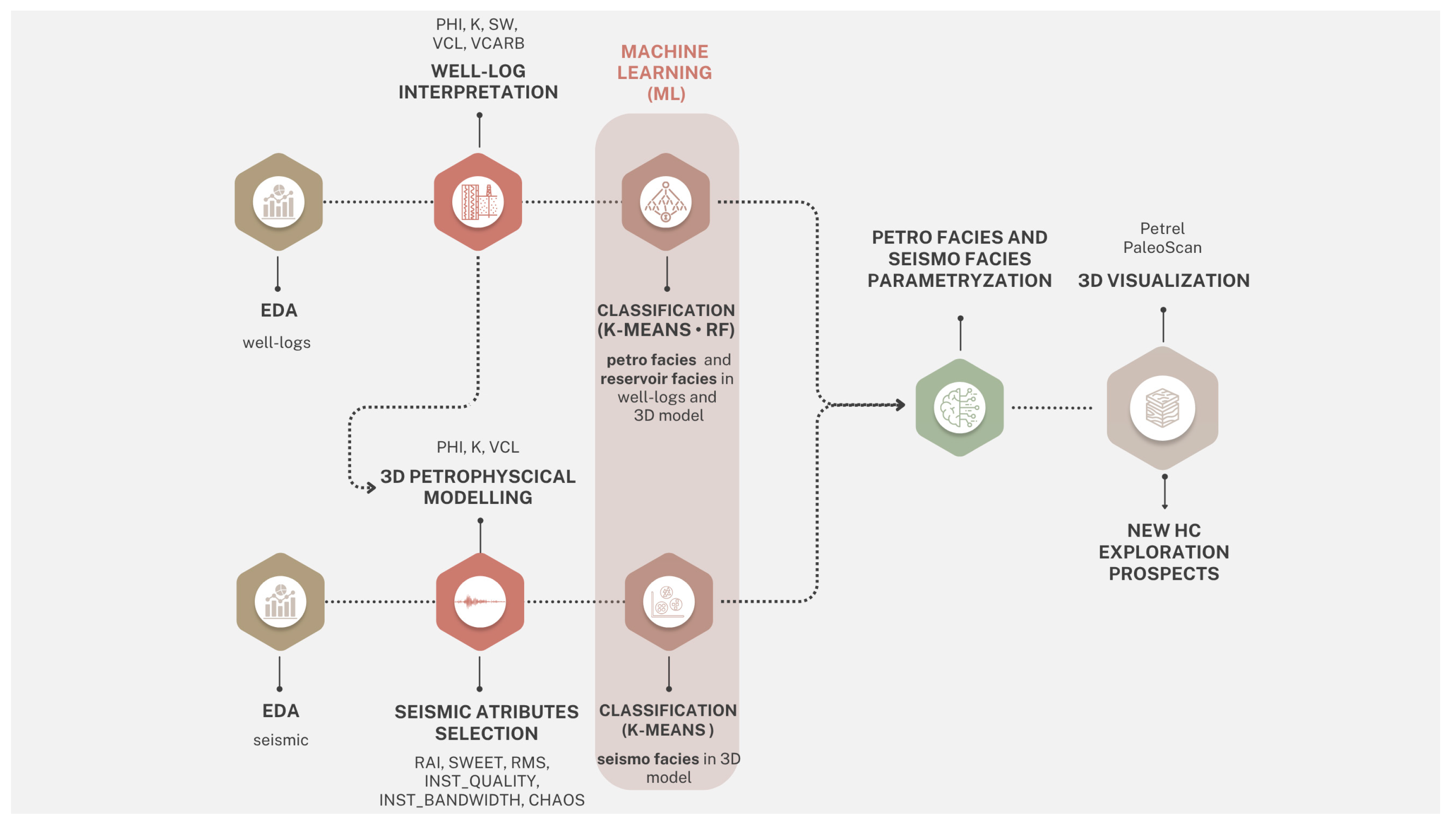
The work was carried out in a few stages (Figure 2). The first stage involved exploratory data analysis (EDA), during which well log and seismic data were prepared for further studies. These data were used for standard geophysical interpretation to determine key reservoir parameters. Additionally, during EDA, well profiles were examined for hydrocarbon indicators observed during well testing. These data served as a training set for RESERVOIR FACIES prediction, characterizing reservoir media and identifying inflow types (or lack thereof) using the random forest (RF) method. Additionally, PETRO FACIES associated with petrophysical and lithological characteristics were identified using the k-means clustering method. These data were also crucial for creating 3D parametric models in the study area.
The random forest method was also employed to predict PETRO FACIES and RESERVOIR FACIES in the 3D model. Simultaneously, work was carried out on selecting seismic attributes that contained information about reservoir, structural, and depositional characteristics. The selected seismic attributes were transformed using the Yeo–Johnson method and subsequently used to create 12 SEISMO FACIES. These seismic facies were parameterized using well data interpretations to identify facies potentially associated with hydrocarbon deposition. The obtained results were visually inspected in Petrel 2023 and PaleoScan 2023 software.

3.1. Data Preparation—Interpretation of Well Log Data

The preparation of well log data for modeling in the Dzików–Uszkowce area focused on deriving essential petrophysical parameters such as clay content, porosity, permeability, irreducible water saturation, and water saturation. The work involved integrating available geological information, including laboratory tests, well test results, NMR measurements, XRD analyses, and stratigraphy. The interpretation was conducted in the Dzików–Uszkowce area and included the 28 boreholes. A full lithological and reservoir interpretation was performed based on a uniform methodology. The list of available well logs and laboratory data in 28 wells is presented in Table 1.
The adopted lithological models were as follows:
  • Clay + Quartz + Carbonates + PHI—for Sarmatian, Upper Badenian, and Lower Badenian formations.
  • Clay + Anhydrite + Gypsum + PHI—for Middle Badenian formations.
Using these models, various reservoir parameters were calculated, including clay content, total porosity (PHIT), calibrated porosity (PHI), effective porosity (PHIE), permeability (K), water saturation (SW), and irreducible water saturation (SWIRR). The mineral content, particularly the presence of carbonates, gypsum, and anhydrite, was also determined through inversion methods and optimization algorithms, which were calibrated against available laboratory data.
Porosity calculations were a key aspect of the interpretation process. Three types of porosity were defined: calibrated porosity (PHI), which was matched with laboratory-measured porosity; total porosity (PHIT), which includes ineffective clay porosity; and effective porosity (PHIE), which is the difference between PHI and the porosity occupied by irreducible water saturation (SWIRR). For old boreholes with limited data, where only neutron was available, porosity adjustments were necessary for gas-saturated intervals, where neutron logs tend to underestimate porosity. To address this issue, the Well Predict procedure was applied, estimating porosity in gas-bearing intervals using data from nearby boreholes.
Clay volume (Vcl) was initially estimated using spectral gamma ray logs (Th-K method), excluding uranium (GRS). Where such logs were unavailable, total natural gamma ray logs were used instead, and the results were calibrated to match mineralogical data from the XRD analysis. One of the key challenges in interpreting Miocene sediments is the reliable determination of effective porosity (PHIE).
Porosity measured by porosimetry and calibrated against wireline log interpretations (PHI) reflects the connected pore space with pore throat diameters above approximately 5 nanometers. This porosity is often relatively high in mudstones, even in zones where perforation tests indicate minimal or no flow of water or gas. This highlights the need to evaluate pore size distribution and identify microporosity (pores in the range of 5–100 nm), which is commonly saturated with irreducible water or gas. Differentiating this component is essential to estimate the volume of movable fluids correctly.
The effective porosity is defined as (1):
PHIE = PHI − PHI × SWIRR
where SWIRR is the irreducible water (and/or gas) saturation within micropores (5–100 nm) PHI is the connected porosity > 5 nm, which includes both effective porosity and porosity filled with irreducible water in micropores
PHIT (total porosity) also includes ultramicropores < 5 nm, typically associated with clay minerals and strongly correlated with Vcl.
The carbonate volume was calibrated either with direct XRD-based carbonate percentages or, more often, with measurements from drill cuttings where core or XRD data were unavailable. Lithological interpretation was supported by empirical relationships between carbonate content and log responses such as photoelectric effect and bulk density that were used as constraints tool in the Quanti ELAN module to give variability of carbonates.
To perform a more integrated interpretation, the Quanti Elan inversion module was applied. This tool solves the petrophysical inverse problem using optimization algorithms. It generates synthetic log responses based on a rock physics model and iteratively adjusts input parameters (such as volume of minerals, porosity, and fluid saturations) to minimize the difference between modeled and measured logs, while honoring laboratory constraints. The following curves were used as an input: GR, DT, RT, RX0, and DT, as well as RHOB if available. The initially calculated VCl, VCARB, and PHI were also used as constraint tools.
In the studied Miocene section, carbonate content typically ranges from ~15% up to 30–35%, while clay content varies broadly from a few percent to approximately 70% and porosity ranges from several percent in claystones to 24–25% in clean sandstones.
Irreducible water saturation and absolute permeability were calculated using the model by Zawisza and Nowak [13] (2) and (3). The calibration constants were set up based on laboratory-measured permeability and irreducible water saturation values
SWIRR = VCL0.22 × (1 − PHI)4
PERM = 35632 × PHIE3.15 × (1 − SWIRR)2
where VCL is the clay volume in the fraction, PHI is the porosity of the fraction, and SWIRR is the irreducible water saturation in the fraction.
These calculations incorporated porosity values adjusted for the micropore fraction, which is particularly important in siltstones and heterolithic deposits, where smaller pore sizes result in lower permeability. For water saturation, Archie’s equation [14] (4) was used in clean sandstone intervals (clay content below 35%). Hill and Milburn [15] found that the relationship between formation water resistivity and rock resistivity is nonlinear due to the clay effect. Therefore, Simandoux [16] (5) or Indonesia [17] (6) equations were applied in siltstone and heterolithic zones, assuming shale resistivity (Rcl) values of 2–3 ohm·m.
The cementation exponent m was measured in the neighboring well. Its values range from 1.7 in claystones to 2 in sandstones. Saturation exponent n ranges from 1.7 in claystones to 2 in clean sandstones. Water resistivity was calculated based on temperature and salinity, which commonly ranges in Miocene deposits from 40 to 55 g/L.
S w = a × R w P H I m × R t
S w S i m = a R w 2 P h i e m V C L R c l + V C L R c l 2 + 4 P H I m a R w R t
S w _ I n d o = 1 R t V C L 1 05 × V c l R c l + P H I m a × R w 2 n
where PHI—effective porosity; Rw—formation water resistivity; Rt—true (uninvaded) formation resistivity from logs; n—saturation exponent; m—cementation exponent; VCL—volume of clay minerals; Rcl—resistivity of clay.
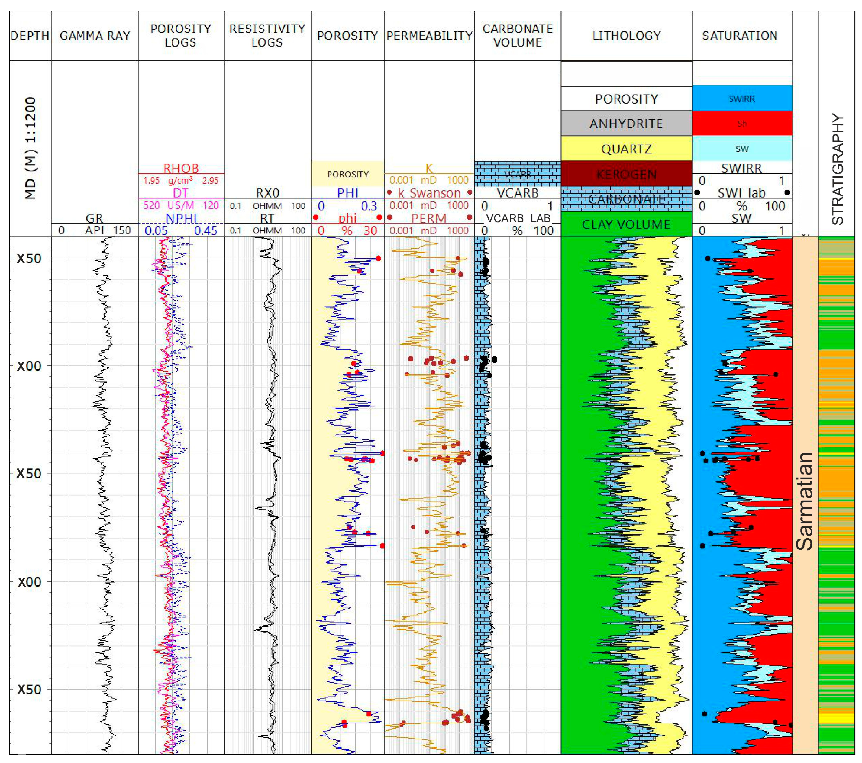
Figure 3 presents the results of well log data interpretation in well DZ-13, calibrated with core-derived parameters such as porosity (PHI), permeability (PERM), carbonate volume, and irreducible water saturation. Figure 4 shows the lithology interpretation in well Z-1, calibrated with XRD data.
The occasionally observed mismatch between the log-derived and core porosity could result from the presence of thin beds. The vertical resolution of the logs is around 50–60 cm, while the heteroliths consist of beds only a few centimeters thick. The logs average the values over several beds.
Based on petrophysical interpretation from 28 wells, four PETRO FACIES were identified using an unsupervised method. These PETRO FACIES allow for a simplified classification of the Miocene deposits, primarily based on clay volume. RT-1 represents clean sandstones, RT-2 corresponds to heteroliths with a predominance of sandstones, RT-3 to heteroliths dominated by mudstones, and RT-4 to a unit composed of mudstones and claystones.
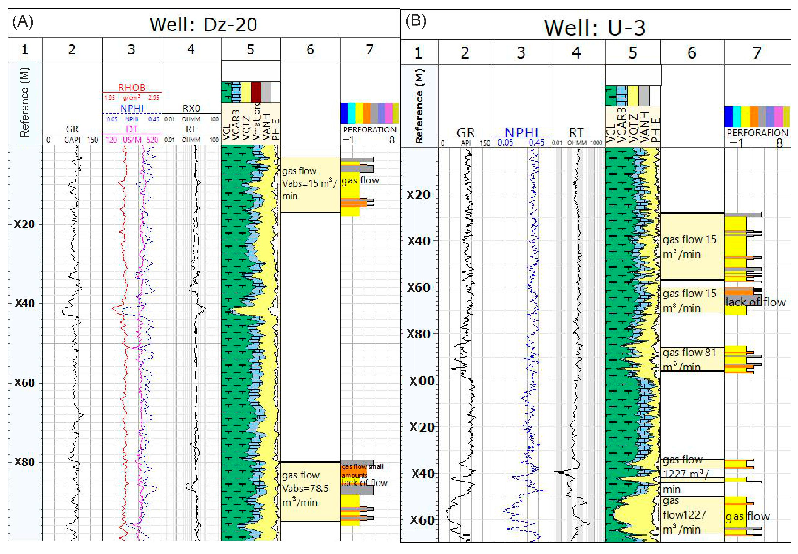
The perforation results were classified into several categories based on gas flow: 0—Heteroliths Water Saturated (HWS), 1—Heteroliths Water and Gas Saturated (HWGS), 2—Heteroliths Gas Saturated (HGS), 3—Heteroliths No Commercial Gas (HNCG), 4—Heteroliths No Flow (HNF), 5—Blocky Sandstones Water Saturated (BSWS), 6—Blocky Sandstones Water and Gas Saturated (BSWGS), 7—Blocky Sandstones Gas Saturated (BSGS). Gas flow was obtained during testing; however, within the tested interval, thin shale interbeds are present. These shales exhibit high gamma-ray log responses, high irreducible water saturation, and low permeability. Even if these layers are water-saturated, no water inflow was observed, as they mainly contain irreducible water. Figure 3 illustrates well log data on tracks 2–4, lithological interpretation on track 5, well test results on track 6, and modified test results on track 7, considering the presence of impermeable and low-permeability thin layers.
Due to the geological complexity of the Dzików–Uszkowce area, traditionally calculated water saturation may be insufficient for some horizons developed as siltstones and heteroliths, requiring advanced techniques and models. In recent years, machine learning algorithms have been successfully applied for this purpose. Methods such as DBSCAN (Density-Based Spatial Clustering of Applications with Noise) and optimally structured multilayer perceptrons (MLPs) can aid in identifying and classifying LRPC zones.
When the layers are very thin, heteroliths occur, which, depending on sandstone and clay mineral content, are classified as sandstone–siltstone heteroliths with dominant sandstones, siltstone–sandstone heteroliths with dominant siltstones, siltstone–claystone heteroliths with dominant siltstones, or claystone–siltstone heteroliths with the poorest reservoir properties, where claystone layers dominate. The presence of clay minerals within the formation causes a reduction in resistivity readings. In horizons developed as heteroliths or siltstones, low resistivity, low contrast (LRLC) zones may occur. Despite gas saturation, resistivity curves in the unaltered zone do not show a clear resistivity increase. Low-resistivity gas horizons (LRLC) exhibit resistivity values comparable to water-saturated zones. Worthington [18] proposed a systematic workflow to interpret LRLC pay zones based on different causes. Li et al. [19] developed a three-step well logging identification method for LRLC zones caused by drilling mud invasion. Pratama et al. [20] introduced an integrated workflow combining petrographical, rock typing, and petrophysical analyses to identify LRLC pay zones. Mashaba and Altermann [21] focused on clay-bound and silt-bound water, improving Archie’s equation for water saturation calculation.
As the water saturation estimates in untested intervals can be particularly uncertain in zones exhibiting low resistivity contrast between hydrocarbon-bearing and water-saturated rocks, the authors focused on developing methodologies for identifying and evaluating Miocene gas-bearing horizons across a range of lithologies—from clean sandstones to mudstones and heterolithic facies. The approach integrates multiple data sources, including well logs, seismic attributes, and perforation results adjusted to account for the presence of sealing and impermeable layers within the analyzed intervals. This issue is illustrated in tracks 6 and 7 of Figure 5.
The detailing of perforation results to reflect changes in the well log data is essential at the data preparation stage. It determines the accuracy of RESEVOIR FACIES predictions in the analyzed area. The results of the saturation prediction algorithm were compared with perforation results and the traditionally calculated water saturation coefficient (SW). Predicted water saturation matched the perforation results and the traditionally calculated water saturation coefficient values in the sandstone intervals. It also indicated potential gas accumulations in mudstone and heterolithic intervals, where the low resistivity contrast between the gas-saturated and water-saturated zones meant that the traditionally calculated water saturation coefficient based on resistivity log data might be unknown or subject to significant uncertainty. The results of well log data interpretation in well Dz-18 are presented in Figure 6.

3.2. Data Preparation—Seismic Analysis

The Uszkowce 3D seismic image, with preserved true amplitude relationships, along with the velocity model utilized to convert the seismic data to the depth domain, were used. The seismic data were a crucial component of the study and were used for construction of the structural model, construction of the computational model (grid), seismic attribute calculation, and construction of the seismic–geological model.

3.3. Structural Model Construction

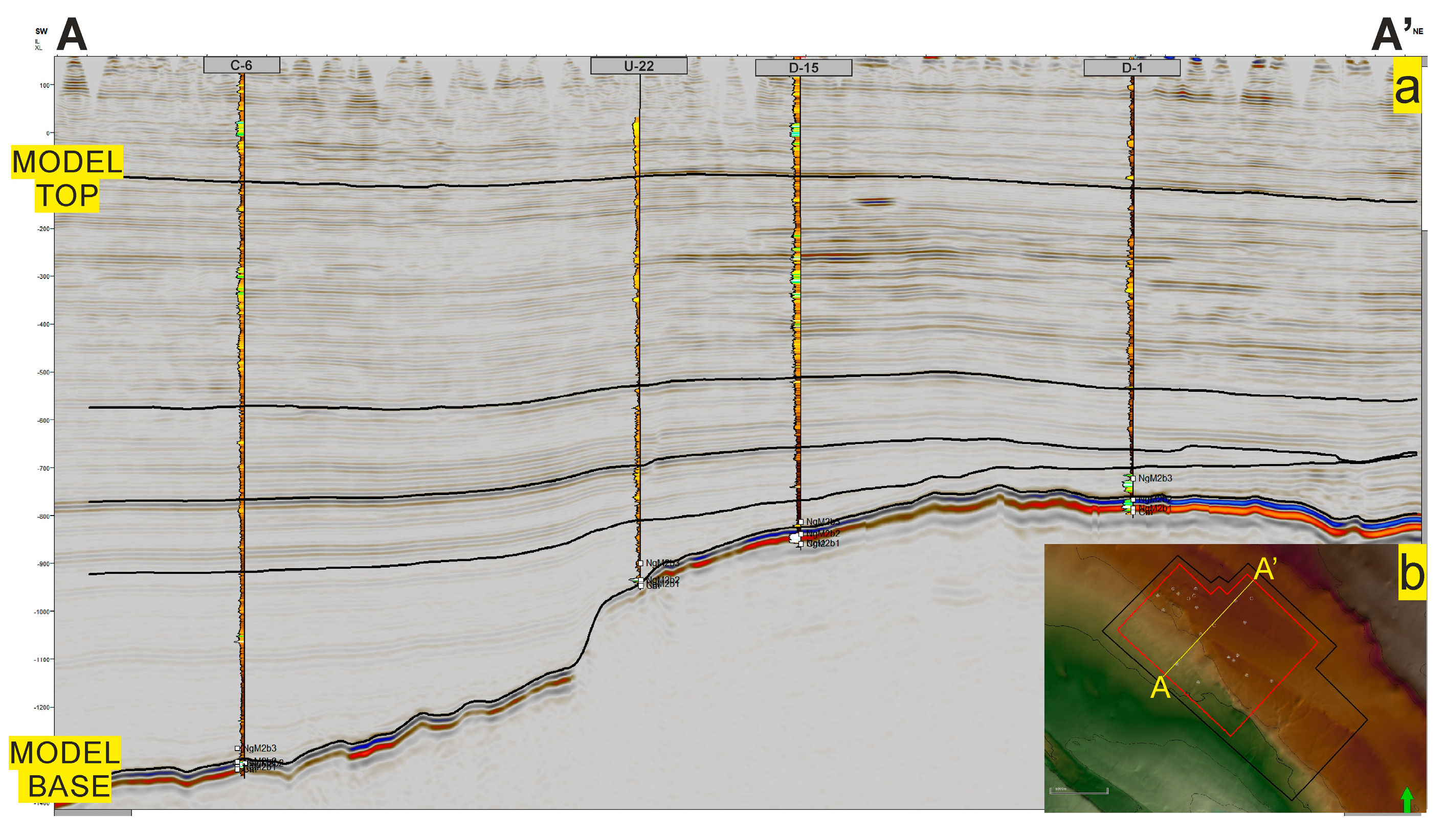
The first step involved defining the structural framework to enable analyses using supervised and unsupervised machine learning algorithms. Due to the quality of the near-surface seismic data, including data gaps caused by acquisition interruptions, and a visible “footprint” artifact related to the geometry of the source and receiver grid during acquisition, it was decided to limit the vertical extent of the model to a depth of −100 m a.s.l. (top model shown in Figure 7). The lower boundary was defined at the first negative phase above the positive phase associated with evaporites, which were not the subject of this analysis. Computational tests indicated that a computational grid not relatively parallel to the seismic phase orientation generates significant errors during both model parameterization and machine learning-based calculations. This issue arises from the complex geological structure of the study area, where the faulted basement influences the basin fill geometry, particularly through drastic variations in the thickness of the Badenian–Sarmatian sedimentary profile. To mitigate such errors, additional internal seismic horizons were defined between the top and base model surfaces (Figure 7). In the model, these surfaces are used to shape the geometry during grid construction and do not correspond to any lithological or stratigraphic markers.

3.4. Seismic Attribute Calculations

The next step in seismic data preparation was the calculation of 16 seismic attributes, which were used in both petrophysical parameterization of the developed model and in analyses employing supervised and unsupervised machine learning algorithms. The calculated attributes are Amplitude contrast, chaos, envelope, first derivative, instantaneous bandwidth, instantaneous frequency, instantaneous phase, instantaneous quality factor, local flatness, original amplitude, reflection intensity, relative acoustic impedance, rms amplitude, second derivative, sweetness, and variance.

3.5. Construction of the Seismo-Geological Model

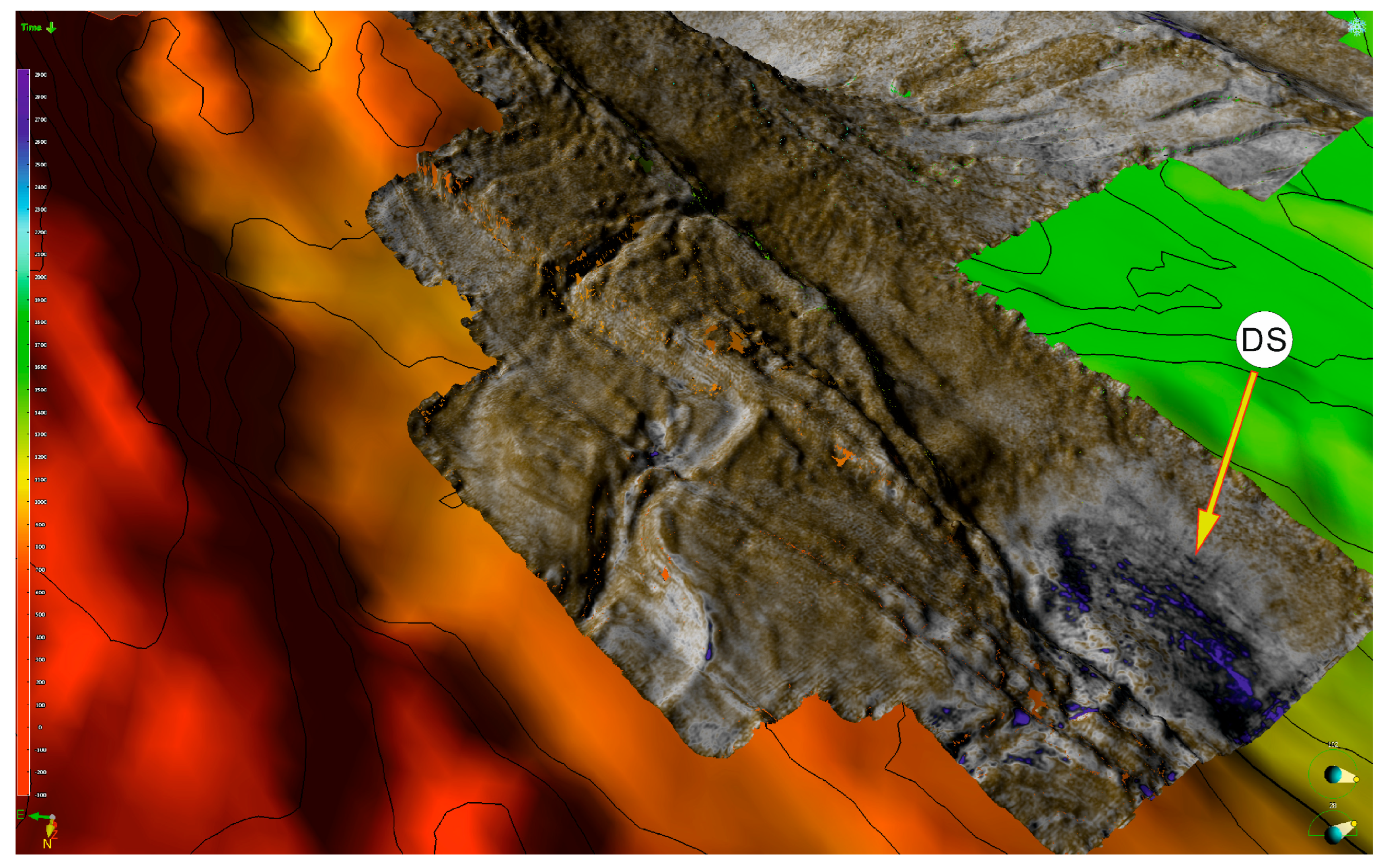
In order to improve the visualization capabilities of machine learning algorithm results, a seismo-geological model was created in Paleoscan software. This software enables the construction of a high-resolution seismo-geological model that takes into account the seismic data sampling step of the 3D seismic data. This results in a multi-layered structural image (seismic horizons) both at the phase maxima and between them. The calculated horizons allow for the analysis of seismic attributes without the intersection cuts of multiple phases, which occur in the case of conventional horizontal seismic sections. Furthermore, the impact of faults is minimized in the interpretation, as the seismo-geological model accounts for the relationships between the hanging and footwall blocks. An example of spatial visualization of the seismo-geological model is presented in Figure 8.

3.6. Prediction of Petro Facies and Hydrocarbon Saturated Zones in Bereholes

The results of borehole geophysical interpretation were used to create PETRO FACIES and RESERVOIR FACIES representing hydrocarbon signs. To predict PETRO FACIES, 4 variables defining reservoir (PHIE, PERM) and lithological (VCL, VCARB) properties were used. Classification was carried out using the k-means method. The k-means method is one of the most commonly used clustering techniques. It utilizes a group of non-hierarchical algorithms aimed at finding and extracting classes of similar objects. Similarity within a defined class should be as high as possible, while differences between classes should be maximized. Several k-means algorithms are available [22]. The standard algorithm is the Hartigan–Wong algorithm [23], which defines the total variability within clusters as the sum of squared Euclidean distances (WSS) between elements and their corresponding centroids. This method requires the prior specification of the expected number of classes. The number of classes was determined arbitrarily to describe the 4 main lithological types with unique petrophysical properties. The optimal number of clusters was also checked using the “elbow” method, which optimizes WSS as a function of the number of clusters (k = 1:15). To predict RESERVOIR FACIES, a random forest classification method (RF) was used. The RF method is based on the random forest algorithm, which is an ensemble of decision trees. Each model (i.e., decision tree) is trained in parallel on a random subset of the training samples and a random subset of input features. Limiting the number of features considered at each split helps prevent a single dominant feature from biasing the model. Each tree in the forest is typically grown to its full depth without pruning, allowing it to capture complex patterns in the data. In classification, each data point is classified by all trees, and the final class is determined by majority voting. This design helps reduce variance, minimize overfitting, and improve prediction quality [24]. This approach differentiates RF from classical bagging, where all variables are used at each split. A unique feature of RF is its ability to find interactions in datasets with many variables, especially those that may have multicollinearity problems. A full description of the mathematical principles of RF algorithms can be found in Louppe [25]. In predicting saturation zones, the RF model was used without tuning the so-called hyperparameters. RESERVOIR FACIES prediction (7 classes) was carried out using 13 variables (DEPTH, PERM, NPHI, PHI, PHIE, PHIT, RT, SW, SWIRR, VCARB, VCL, VQRTZ, PETRO FACIES). Due to the limited number of observations in classes 5 and 6 (BSWS and BSWGS), these classes were merged into a single class—BSWGS (now designated as class 5). Additionally, class 7 (BSGS) was reassigned to class 6. The final class arrangement is as follows: 0—Heteroliths Water Saturated (HWS); 1—Heteroliths Water and Gas Saturated (HWGS); 2—Heteroliths Gas Saturated (HGS); 3—Heteroliths No Commercial Gas (HNCG) (up to 10 m3/min); 4—Heteroliths No Flow (HNF); 5—Blocky Sandstones Water and Gas Saturated (BSWGS); 6—Blocky Sandstones Gas Saturated (BSGS). The training and test datasets were split in an 80/20 ratio. Modeling was conducted in the RStudio (2024.04.2) environment using the tidymodels meta-package and the latest machine learning concepts developed by the R Core Team [26,27]. Due to the highly imbalanced nature of the classes (sandstone and gas-saturated heteroliths are in the minority), bootstrapping was applied during modeling. This technique involves creating balanced datasets through resampling with replacement, which can be achieved, for example, by oversampling the minority class. Additionally, stratification was used to enforce proportional distribution of classes in both subsets (training and test). In the data preparation process, techniques for normalizing continuous data (centering and scaling) and the SMOTE algorithm (Synthetic Minority Oversampling Technique) were also used. SMOTE is used to handle the problem of imbalanced classes by generating synthetic samples for the minority class. The algorithm automatically detects underrepresented classes in the outcome variable and generates new data for the minority class by interpolating between existing examples of that class. This is carried out based on k-nearest neighbors (default is 5). After applying the algorithm, a balanced dataset is obtained, where the minority class has more observations due to the added synthetic samples. Bootstrapping, stratification, and the SMOTE algorithm are commonly used to improve model performance and address the issue of imbalanced classes in machine learning [26]. A detailed description of models with a list of variables, pre-processing, and tuning strategy was listed in Table 2.

3.7. Parametric Modeling

It was necessary to develop a structural framework in the form of a computational grid model based on 3D seismic data in order to apply supervised and unsupervised machine learning algorithms. The grid model has dimensions (width x, width y, thickness z): 50 m × 50 m × 5 m and a total of 29.3 million cells. This resolution, aligned with the average vertical resolution of the seismic data (~9 m), allowed for a satisfactory division of the seismic volume into individual computational cells. Combined with the high-resolution seismo-geological model (PaleoScan), it enabled a very precise analysis of the obtained results. The next step was model parameterization based on the interpretation of well log data. This part was used during calculations involving supervised machine learning algorithms. Three parameters were computed: clay content (VCL)—average value: 45%; effective porosity (PHIE)—average value: 14.8%; permeability (PERM)—average value: 5 mD. Figure 9 and Figure 10 present the spatial results of the parameterization. A clear presence of sandy lithosomes is observed in the basal part of the model, characterized by good petrophysical properties.

3.8. Three-Dimensional Seismic Facies Prediction

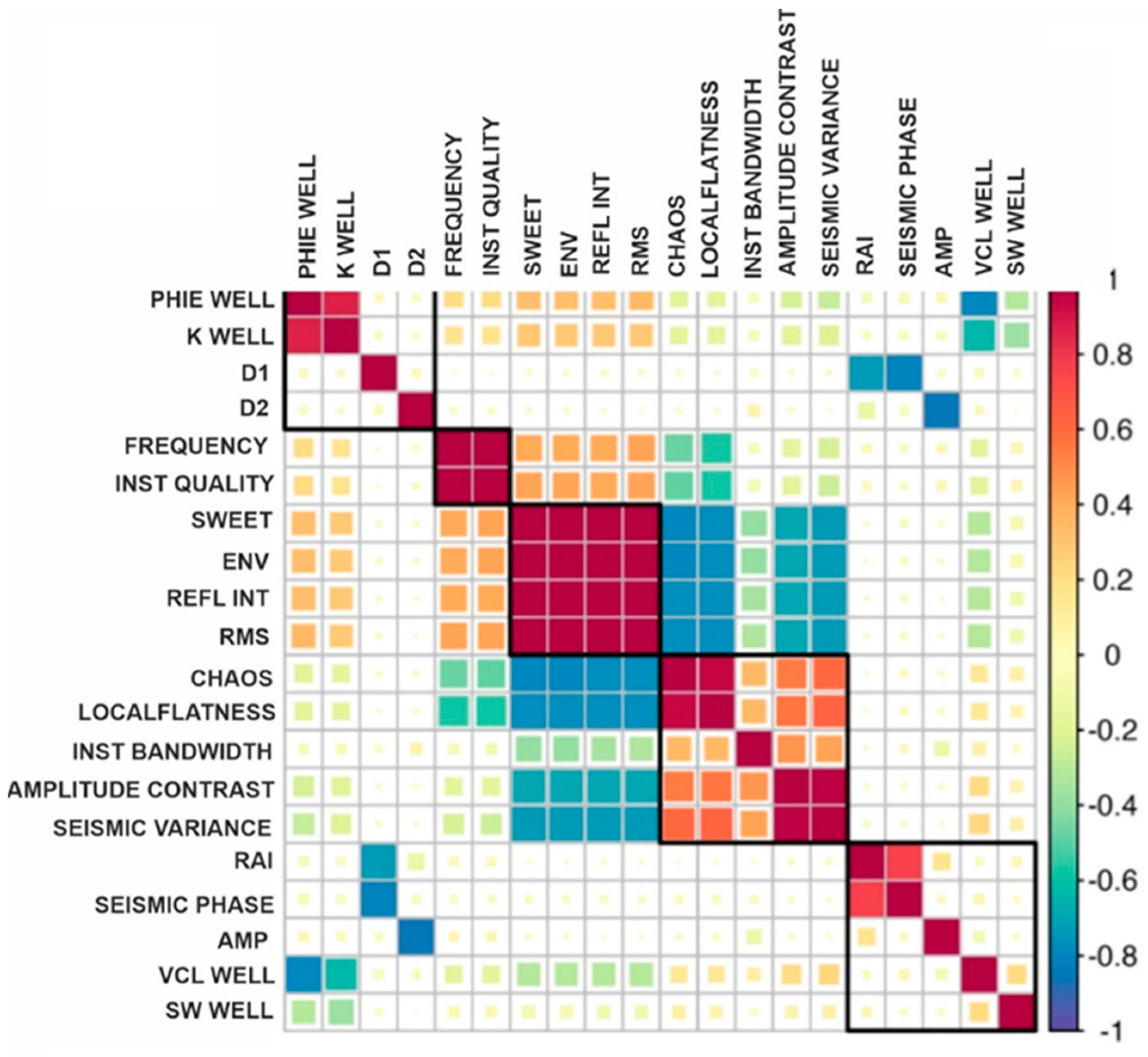
The 3D seismic PETRO FACIES and RESERVOIR FACIES were predicted using a similar approach. Due to the limited number of observations characterizing outcome variables, after the upscaling procedure of classes, it was decided to skip the division into training and testing datasets and instead apply bootstrapping on 200 subsets (resampling), where both training and evaluation sets were included. Stratification and the SMOTE algorithm were also applied in this case. For PETRO FACIES and RESERVOIR FACIES prediction, RF was used after hyperparameter tuning. Hyperparameters in machine learning are model parameters that are set before the learning process begins and are optimized during the training phase. They are important for the performance of the model and its ability to generalize. The RF algorithm requires the definition of three hyperparameters before the modeling process starts: mtry—the number of variables considered at each split; trees—the number of trees in the ensemble (forest); and min_n—the minimum number of observations in a node required for further splitting. Detailed information on the hyperparameters of the random forest algorithm can be found in Boehmke and Greenwell [22]. Hyperparameter tuning was performed using the tune race ANOVA method, testing 200 models in 20 different combinations. This method calculates the accuracy metric value for selected hyperparameters (mtry, trees, and min_n) based on the results from subsets of data. The algorithm tests the statistical significance of hyperparameter combinations and eliminates those that are not promising using the ANOVA model [28]. PETRO FACIES prediction was performed using 20 variables integrating seismic attributes and information about porosity, permeability, and clay content (AMP, SEISMIC_PHASE, RAI, SEISMIC_VARIANCE, AMPLITUDE_CONTRAST, INST_BANDWIDTH, LOCAL_FLATNESS, CHAOS, RMS, REFL_INT, ENV, SWEET, INSTANT_QUALITY, FREQUENCY, D1, D2, PHIE, K, AND VCL). For RESERVOIR FACIES prediction, the same set of attributes was applied together with predicted PETRO FACIES (Table 2). Additionally, 6 seismic attributes were selected (RAI, SWEET, RMS, INST_QUALITY, INST_BANDWIDTH, CHAOS) that may assist in the characterization of depositional systems, bearing specific structural, lithological, and reservoir characteristics. These attributes were used to create 12 SESISMO FACIES using the k-means method. This unsupervised learning method is an excellent alternative for analyzing 3D seismic data with limited traditional structural interpretation, allowing for the identification of features [29]. This method provides fast results and is often recommended for analyzing large seismic datasets (~10 million cells). Attribute selection was performed using the correlation matrix shown in Figure 11. The figure illustrates the relationships between seismic attributes and reservoir parameters (PHI, PERM, VCL, SW) in the interpreted boreholes. The correlation between reservoir parameters and seismic attributes deviates from linear relationships, as expressed by a low Spearman correlation coefficient, making the prediction of these parameters from seismic data challenging. Additionally, in Figure 11, attributes with high correlation were grouped using hierarchical clustering and the Lance–Williams divergence update formula with Ward’s method. This method uses the classical sum of squares criterion to create groups that minimize within-group dispersion [30,31,32]. The number of clusters was arbitrarily set to 6 in order to select 6 seismic attributes for further analysis.
The selected attributes were transformed using the Yeo–Johnson method. The Yeo–Johnson transformation extends the Box–Cox transformation concept, allowing for the transformation of data that can be both positive and negative [33]. This method stabilizes variance and improves the symmetry of the distribution, which is important during clustering.

4. Results and Discussion

4.1. Prediction of PETRO FACIES and RESERVOIR FACIES in Well Logs

The classification model achieved a strong overall performance, reaching 91% accuracy on the test set. The evaluation metrics highlight excellent precision and recall for most facies, with only one class showing notable room for improvement.
Heteroliths Water Saturated (HWS), Heteroliths Water and Gas Saturated (HWGS), and Blocky Sandstones Water and Gas Saturated (BSWGS) were classified with near-perfect precision and recall (all ≥ 0.99) (Table 3). Blocky Sandstones Gas Saturated (BSGS) also demonstrated excellent performance, achieving a 0.95 F1 score, supported by a high recall (0.97). Similarly, Heteroliths Gas Saturated (HGS) were reliably identified, though the slightly lower recall (0.90) indicates occasional misclassification.
The most challenging class for the model was Heteroliths No Commercial Gas (HNCG), which obtained a precision of 0.60 and F1 score of 0.69. The confusion matrix reveals significant overlap with HGS and HNF, suggesting these facies share similar petrophysical responses that complicate discrimination.
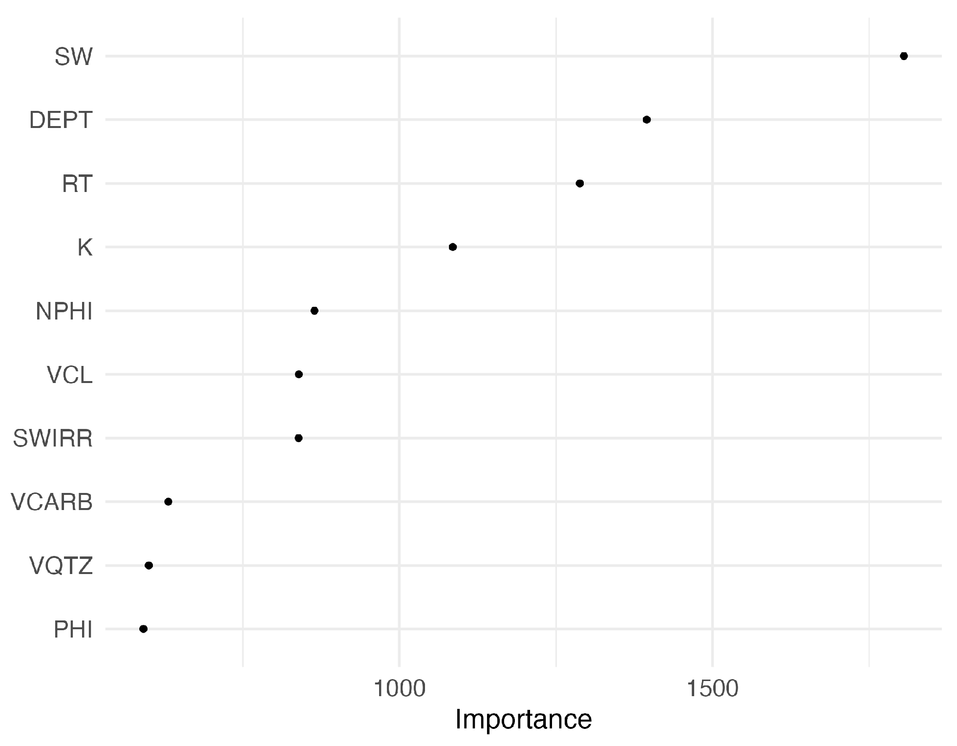
Feature importance analysis reveals water saturation (SW) as the most influential predictor, followed by depth (DEPT), resistivity (RT), and permeability (K) (Figure 12). These features align well with geological expectations, as they are critical for identifying fluid types and flow potential in reservoir rocks. Neutron porosity (NPHI), volume of clay (VCL), and irreducible water saturation (SWIRR) also contribute meaningfully, supporting the differentiation of heterolithic facies.
The obtained results were compared with the results of perforations and the traditionally calculated water saturation coefficient (SW). The predicted saturations matched the described perforation results and the traditionally calculated water saturation coefficient values in the sandstone intervals. At the same time, they indicated potential gas accumulations in the mudstone and heterolith intervals, where there is a low resistivity contrast between the gas-saturated and water-saturated zones. In these intervals, the traditionally calculated water saturation coefficient, based on resistivity logs, can be subject to significant uncertainty.

4.2. Prediction of PETRO FACIES in the 3D Model

The multiclass model with imbalanced classes for PETRO FACIES prediction was evaluated using the same set of metrics. The classification model for PETRO FACIES prediction achieved an overall mean accuracy of 80% (SD = 0.01) across the validation set. This demonstrates a robust capability to distinguish between the four rock types (RT1–RT4), although some variability in class-specific performance is evident.
RT1 (Clean Sandstones) exhibited the lowest precision (0.70) and recall (0.65) with relatively high standard deviations (SD = 0.16 and 0.18, respectively), leading to an F1 score of 0.65 (SD = 0.13) (Table 4). The confusion matrix indicates significant misclassification of RT1 samples as RT2, reflecting the geological similarity between clean sandstones and heteroliths dominated by sandstones (Figure S1).
RT2 (Heteroliths with Sandstone Dominance) performed strongly, achieving a precision of 0.82 (SD = 0.04), recall of 0.88 (SD = 0.03), and F1 score of 0.85 (SD = 0.02). While occasional misclassification into RT3 is observed, this unit remains reliably identified overall.
RT3 (Heteroliths Dominated by Mudstones) showed balanced metrics with precision of 0.82, recall of 0.78, and F1 score of 0.80 (all with very low SD). However, some samples were confused with RT4, which is consistent with their transitional petrophysical properties.
RT4 (Mudstones and Claystones) demonstrated solid performance with precision and recall near 0.78–0.80. The confusion matrix suggests minor overlap with RT3, but the classifier successfully captures the primary characteristics of this unit (Figure S2).
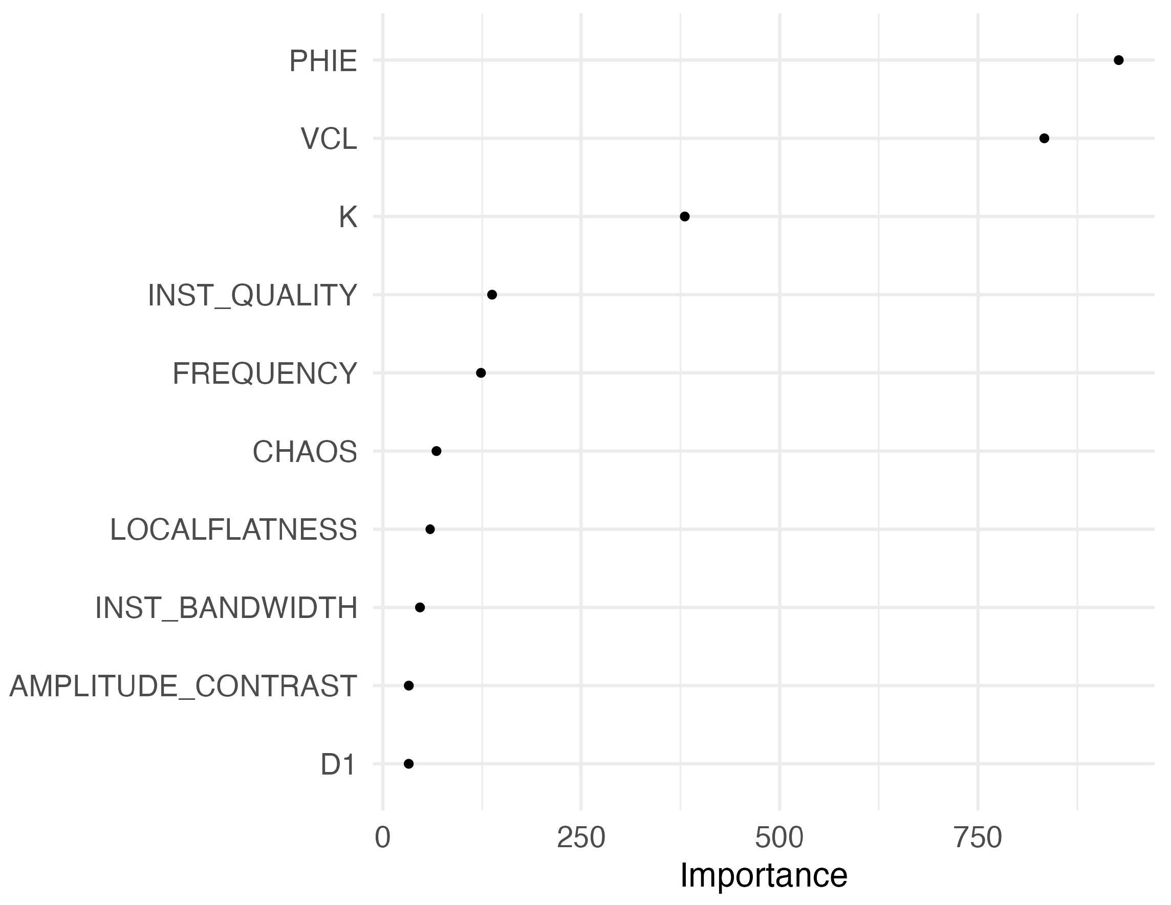
Feature importance analysis reveals PHIE (effective porosity) as the dominant variable, followed by VCL (volume of shale) and PERM (permeability), highlighting the key role of petrophysical attributes in class differentiation (Figure 13). Seismic attributes such as INST_QUALITY, FREQUENCY, and CHAOS also contribute significantly, aiding in the discrimination of texturally complex heteroliths.

4.3. Prediction of RESERVOIR FACIES in the 3D Model

Predicting the presence of hydrocarbons turned out to be the most difficult task for the analyzed model. The classification model achieved an overall mean accuracy of 70% (SD = 0.01) on the validation set. While this indicates a reasonable predictive performance, the class-level metrics reveal substantial variability across facies types.
Blocky Sandstones Water and Gas Saturated (BSWGS) and Heteroliths Water and Gas Saturated (HWGS) showed the strongest performance, with F1 scores of 0.81 and 0.74, respectively (Table 5). Both facies were consistently predicted with high precision (BSWGS: 0.81; HWGS: 0.70) and recall (BSWGS: 0.81; HWGS: 0.78). Heteroliths No Flow (HNF) also demonstrated robust metrics, with a precision of 0.82, recall of 0.84, and F1 score of 0.83, reflecting reliable identification of non-productive zones.
In contrast, Blocky Sandstones Gas Saturated (BSGS) and Heteroliths No Commercial Gas (HNCG) were particularly challenging for the model. BSGS exhibited very low precision (0.11) and recall (0.05), resulting in a poor F1 score of 0.08. HNCG performed similarly poorly (F1 score: 0.03), with frequent misclassification into HNF and HWGS, as revealed by the confusion matrix (Figure S3). Heteroliths Gas Saturated (HGS) also struggled, with an F1 score of only 0.12, driven by low recall (0.07).
The feature importance plot highlights PERM (permeability) as the most influential predictor, followed by PHIE (effective porosity) and VCL (volume of shale) (Figure 14). These petrophysical parameters are critical for differentiating hydrocarbon-bearing facies from water-saturated and non-productive intervals. Seismic attributes, such as INST_QUALITY and FREQUENCY, provide additional discrimination power but contribute less overall.
While the model reliably distinguishes water-saturated and mixed facies (BSWGS, HWGS, HNF), its difficulty in identifying pure gas-saturated units (BSGS and HGS) suggests the need for another approach for hydrocarbon facies detection

4.4. Seismic Facies Parametrization

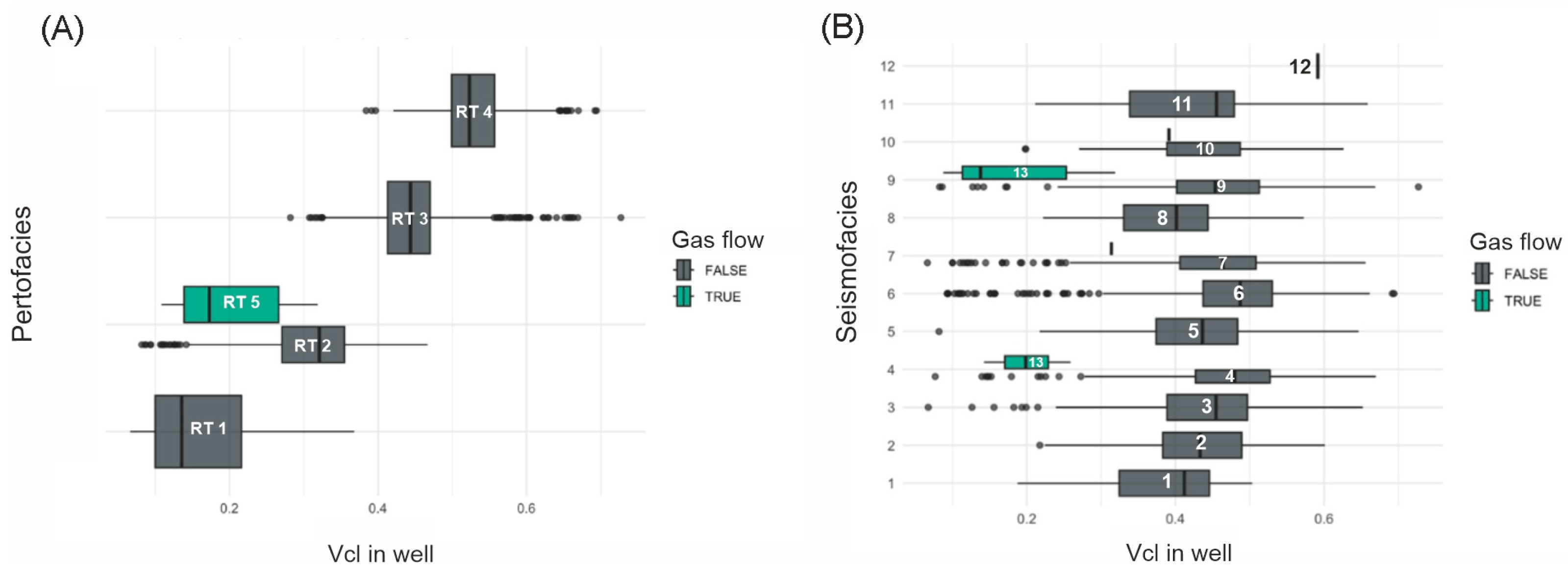
In terms of SEISMO FACIES analysis, the study successfully identified 12 seismic facies using selected seismic attributes, and an additional class of facies (facie 13) was defined to indicate gas-saturated zones. This new class helps differentiate gas-saturated sandstones with high accumulation potential, providing valuable insights for further exploration. To determine additional classes, information on hydrocarbon-bearing zones and clay volume in the boreholes was used (Figure 15). Additional facies within the PETRO FACIES and SEISMO FACIES were determined using two model variants: (a) using the cutoff of 0.3 VCL and filtering facie 11 in the PETRO FACIES and facies 9 and 4 in the SEISMO FACIES, leaving only those cells in which gas was found.

4.5. Spatial Results Analysis

A spatial analysis of the results of supervised and unsupervised machine learning algorithms was presented for the two variants:
  • Unsupervised SEISMO FACIES, 13 classes, class No. 13—Gas-Saturated Sandstones;
  • Supervised PETRO FACIES, 5 classes: RT1—Clean Sandstones; RT2—Heteroliths with Sandstone Dominance; RT3—Heteroliths Dominated by Mudstones; RT4—Mudstones and Claystones; RT5—Gas-Saturated Sandstones.
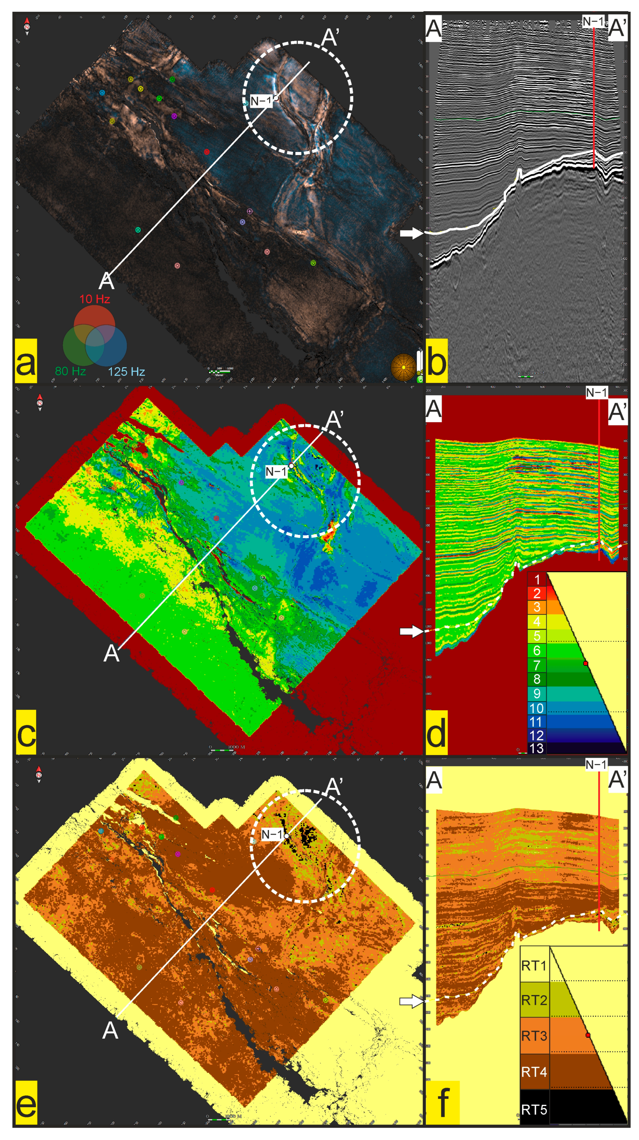
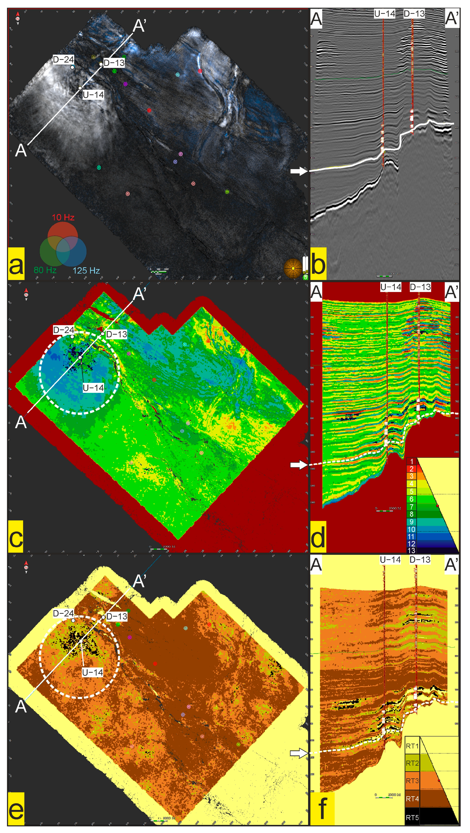
The results of the calculations, using the above-presented models, for four seismic surfaces representing the Badenian–Sarmatian sedimentary succession, calculated within the seismo-geological model, are presented below. They were selected due to several interesting features that can be observed within them: (1) depositional architecture, (2) the possibility of observing changes in the sedimentary basin on its basis, and (3) the results of saturation prediction. Figure 16 and Figure 17 have the following fixed structure:
  • a—result of spectral decomposition with a visible course of the seismic profile from panels B, D, and F (blue line);
  • b—seismic profile with a visible position of the seismic horizon presented in panels a, c, e (yellow line);
  • c—result of the SEISMO FACIES model;
  • d—profile (analogous position as in b and f) representing the result of the SEISMO FACIES model;
  • e—result of the PETRO FACIES model;
  • f—profile (analogous position as in b and d) representing the result of the PETRO FACIES model.
Figure 16 presents the oldest of all the discussed surfaces. It represents the stratigraphic interval: upper Badenian–lower Sarmatian contact. The analyzed object is a sandy lithosome located just above the evaporite level in the northern part of the seismic section. It was drilled using boreholes D-1, D-2, and N-1, which resulted in a commercial gas inflow. The N-1 well was not used in the parameterization process of the model nor the supervised machine learning algorithms. Therefore, it allowed for independent validation of the obtained results against the geological conditions confirmed by this well.
The described supra-evaporite interval is characterized by very high variability in the observed depositional elements. A meandering network of wide channels dominates, suggesting a high-energy environment responsible for their formation. These channels transported platform-derived material from the north toward the basin center. This interpretation is supported by regional analysis of the 3D seismic data as well as the petrographic composition of Dzików sandstones, which are relatively coeval with the described lithosome. The course of the channels was most likely controlled by the morphology of the underlying strata, which at that time was affected by faulting (reactivation of older faults). This is indicated by the alignment of depositional directions with the orientation of these dislocations. Its spatial geometry is also clearly reflected in the results of the SEISMO and PETRO FACIES predictions (Figure 16c,e). These are consistent with the spectral decomposition image (Figure 16a). The analysis of the compiled results allows for the following conclusions:
The imaging of the geometry of depositional architecture seems to be more effective when using unsupervised SEISMO FACIES prediction expressed through 12 classes (class 13—gas-saturated zones—dark navy blue). Applying an appropriate color scale allows for a more detailed and diverse image, even compared to that from spectral decomposition. Unfortunately, in this case, class 13, which is associated with saturation, was not observed in the location where the N-1 well confirmed the presence of hydrocarbons.
The PETRO FACIES prediction results, which also include gas-saturated zones (RT 5—gas-saturated zones—black color), unlike the SEISMO FACIES, show a positive correlation between the presence of class 5 and the occurrence of gas in borehole N-1. This is an important result, confirming the effectiveness of the applied research methodology. Moreover, the distribution of PETRO FACIES 1 and 2 confirms the sandy nature of the described interval (based on data from N-1, D-1, -2 boreholes).
Figure 17 presents the results of SEISMO and PETRO FACIES predictions for the first of the Dzików sandstone levels. Unlike the previously described interval, this one is assigned to the lower part of the Lower Sarmatian, marked by the appearance of foraminifera from the Anomalinoides dividens group (the result of microfaunal analyses from the “Dz” boreholes). These sandstones, of platform origin, occur in the form of four levels whose sedimentation was controlled by the structural development of the substratum. Their characteristic form resembles depositional lobes with variable extents (the oldest–widest distribution; the youngest–smallest), located directly south of the fault that bounds the Lubaczów uplift from the south. This coincidence may indicate short-distance transport of material, which resulted in the incision of a shallow, pelagic shelf. The limiting factor of this process (reducing the transport energy) was a threshold in the substrate of the sedimentary basin. The described depositional system is visible both in the spectral decomposition results and in the outcomes of the PETRO and SEISMO FACIES models (Figure 17).
Interpretation of this seismic section is facilitated by numerous boreholes related to natural gas accumulations in the Dzikow and Uszkowce area. A particularly interesting case involves two neighboring boreholes (1300 m apart) located south of the fault zone: U-14 and Dz-24. In the U-14 borehole, gas inflow from the Dzików sandstones was observed, and this borehole was used in the PETRO and SEISMO FACIES predictions. In contrast, the Dz-24 borehole, which drilled through an analogous depositional sequence to that of U-14, was water-saturated despite a structurally more favorable position. It is important to note that U-14, unlike Dz-24, was used in the prediction process. This methodological approach is analogous to the N-1 case, allowing for model validation against borehole results that did not contribute training data to the machine learning algorithms.
Based on the analysis of the example shown in Figure 17, the following conclusions can be drawn:
  • A positive correlation was obtained for gas-saturated zones in both the Dz-24 and U-14 boreholes in the SEISMO and PETRO FACIES models. Classes 13 (SEISMO FACIES—dark navy blue) and 5 (PETRO FACIES–black) are observed around U-14, while they are absent near Dz-24.
  • A strong correlation was observed between the spectral decomposition image and the results of the SEISMO and PETRO FACIES models. The compiled dataset accurately reflects the depositional architecture in the form of depositional lobes with varying spatial extent.
The PETRO FACIES model logically and consistently reflects lithological information from the boreholes, illustrating the facies’ transition as a function of transport distance. The further from the axis of channelized transport of Dzikow sandstones (north of the aforementioned fault), the more sandstones are replaced by heteroliths and mudstones. This interpretation is supported by the relation between the U-14 and C-6 boreholes. The C-6 well, located 4700 m southeast of U-14, records a decrease in sand content, which correlates with the lowermost, thick Dzików sandstone present in U-14 and Dz-24.

5. Summary and Conclusions

This study focuses on predicting petrophysical facies and RESERVOIR FACIES in boreholes and extending these predictions into a 3D geological model using machine learning methods. Random forest classifiers, applied to well log and seismic data, demonstrated strong performance in PETRO FACIES prediction, achieving an accuracy of 80% (SD = 0.01) in the 3D model and effectively distinguishing sandstone- and mudstone-dominated facies. RESERVOIR FACIES classification, covering seven hydrocarbon system classes, showed moderate overall accuracy (70 ± 1%) but revealed significantchallenges in identifying gas-saturated zones. Gas-bearing facies such as Blocky Sandstones Gas Saturated (BSGS) and Heteroliths Gas Saturated (HGS) exhibited very low F1 scores (0.08 and 0.12, respectively) and recall values below 7%, indicating limited sensitivity to minority classes and significant misclassification into water-saturated or non-productive facies.
The SEISMO FACIES analysis provided an additional layer of interpretation by identifying 12 distinct seismic facies from key attributes and defining a new facies to highlight gas-saturated sandstones with high accumulation potential. This approach successfully differentiated lithological and fluid-related heterogeneities at the seismic scale. Importantly, a strong spatial correlation was observed between SEISMO FACIES (facies 13) and PETRO FACIES (RT5) predictions in the 3D model, particularly in the validation boreholes. At N-1, both models consistently predicted gas-bearing zones, which were confirmed by well test results. Similarly, Dz-24 showed an absence of hydrocarbon indicators in both PETRO FACIES and SEISMO FACIES, aligning with the dry hole outcome. This agreement underscores the integrated model’s reliability for predicting the presence of hydrocarbons in areas with sparse well control.
These results highlight the high potential of machine learning, particularly random forest models, for predicting lithofacies and hydrocarbon indicators in complex geological settings. Incorporating additional well log parameters, such as photoelectric factor (PE) and compressional slowness (DT), may further enhance lithotype and saturation predictions. Moreover, integrating depositional sequence frameworks within wells could provide a more robust link between petrophysical and seismic facies, facilitating improved spatial extrapolation of reservoir properties and aiding exploration in underexplored areas.

Supplementary Materials

The following supporting information can be downloaded at: https://www.mdpi.com/article/10.3390/en18174521/s1, Figure S1: FLOW_TYPE well logs confusion_matrix; Figure S2: PETROFACIES confusion_matrix; Figure S3: FLOW_TYPE confusion_matrix.

Author Contributions

Conceptualization, D.A. and T.T.; methodology, D.A., T.T., L.-Ś.A. and S.K.; software, D.A., T.T., L.-Ś.A. and S.K.; validation, D.A., T.T., L.-Ś.A. and S.K.; formal analysis, D.A. and T.T.; investigation, D.A. and T.T.; resources, D.A., T.T., L.-Ś.A. and S.K.; data curation, D.A. and T.T., L.-Ś.A. and S.K.; writing—original draft preparation, D.A., T.T. and L.-Ś.A.; writing—review and editing, D.A., T.T. and L.-Ś.A.; visualization, D.A., T.T. and L.-Ś.A.; supervision, D.A. and T.T.; project administration, L.-Ś.A.; funding acquisition, D.A., T.T., S.K. and L.-Ś.A. All authors have read and agreed to the published version of the manuscript.

Funding

This research was funded (1) by the Ministry of Science and Higher Education, Grant no. DK-4100-23/24. The authors would like to express their gratitude to the Polish Ministry of Science and Higher Education for funding this research and the (2) Ministry of Science and Higher Education, financing the implementation doctorate entitled: “Stratigraphy forward modeling of sedimentary processes in autochthonous Miocene formations of the eastern part of the Carpathian Foredeep”, carried out at the AGH Doctoral School.

Data Availability Statement

The data supporting the findings of this research are available on reasonable request from the corresponding author.

Conflicts of Interest

The authors declare no conflicts of interest.

References

  1. Dziadzio, P. Sekwencje depozycyjne w utworach badenu i sarmatu w SE części zapadliska przedkarpackiego. Prz. Geol. 2000, 48, 1124–1138. [Google Scholar]
  2. Dziadzio, P.; Maksym, A.; Olszewska, B. Sedymentacja utworów miocenu we wschodniej części zapadliska przedkarpackiego. Prz. Geol. 2006, 54, 413–420. [Google Scholar]
  3. Antariksa, G.; Muammar, R.; Lee, J. Performance evaluation of machine learning-based classification with rock-physics analysisof geological lithofacies in Tarakan Basin, Indonesia. J. Pet. Sci. Eng. 2022, 208, 109250. [Google Scholar] [CrossRef]
  4. Feng, R. Improving uncertainty analysis in well log classification by machine learning with a scaling algorithm. J. Pet. Sci. Eng. 2021, 196, 107995. [Google Scholar] [CrossRef]
  5. Wang, P.; Chen, X.; Wang, B.; Li, J.; Dai, H. An improved method for lithology identification based on a hidden Markov model and random forests. Geophysics 2020, 85, IM27–IM36. [Google Scholar] [CrossRef]
  6. Okpoli, C.C.; Arogunyo, D.I. Integration of Well Logs and Seismic Attribute Analysis in Reservoir Identification on PGS Field Onshore Niger Delta, Nigeria. Pak. J. Geol. 2020, 4, 12–22. [Google Scholar] [CrossRef]
  7. Pietsch, K.; Jarzyna, J. Identification of Miocene gas deposits from seismic data in the southeastern part of the Carpathian Foredeep. Geol. Q. 2002, 46, 449–461. [Google Scholar]
  8. Łukaszewski, M. The application of volume texture extraction to three-dimensional seismic data—Lithofacies structures exploration within the Miocene deposits of the Carpathian Foredeep. Geol. Geophys. Environ. 2020, 46, 301–313. [Google Scholar] [CrossRef]
  9. Myśliwiec, M. Traps for gas accumulations and the resulting zonation of the gas fields in the Miocene strata of the eastern part of the Carpathian Foredeep (SE Poland). Przegląd Geol. 2004, 52, 657–664. [Google Scholar]
  10. Oszczypko, N.; Ślączka, A. The evolution of the Miocene Basin in the Polish Outer Carpathian and their foreland. Geol. Carpathica 1989, 40, 23–36. [Google Scholar]
  11. Ney, R.; Burzewski, W.; Bachleda, T.; Górecki, W.; Jakóbczak, K.; Słupczyński, K. Outline of paleogeography and evolution of lithology and facies of Miocene layers on the Carpathian Foredeep. Pr. Geol. 1974, 82, 1–65. [Google Scholar]
  12. Porębski, S.J.; Warchoł, M. Znaczenie przepływów hiperpyknalnych i klinoform deltowych dla interpretacji sedymentologicznych formacji z Machowa (miocen zapadliska przedkarpackiego. Przegląd Geol. 2006, 54, 421–429. [Google Scholar]
  13. Zawisza, L.; Nowak, J. Metodyka określania parametrów filtracyjnych skał na podstawie kompleksowej analizy danych geofizyki otworowej; Wydawnictwa AGH: Kraków, Poland, 2012; pp. 106–115. ISBN 978-83-7464-497-6. [Google Scholar]
  14. Archie, G.E. The Electrical Resistivity Log as an Aid in Determining Some Reservoir Characteristics. Trans. AIME 1942, 146, 54–62. [Google Scholar] [CrossRef]
  15. Hill, H.J.; Milburn, J.D. Effect of clay and water salinity on electrochemical behavior of reservoir rocks. Trans. AIME 1956, 207, 65e72. [Google Scholar] [CrossRef]
  16. Simandoux, P. Mesures Dielectriques en Milieu Poreux, Application à la Mesure des Saturations en Eau, Etude du Comportement des Massifs Argileux. Rev. L’institut Français Pétrole 1963, 18, 193–215. [Google Scholar]
  17. Poupon, A.; Leveaux, J. Evaluation of Water Saturation in Shaly Formations. In Proceedings of the 12th Annual SPWLA Symposium, Dallas, TX, USA, 2–5 May 1971. Society of Petrophysicists and Well Log Analysts. [Google Scholar]
  18. Worthington, P.F. Recognition and development of low-resistivity pay. In Proceedings of the SPE, Asia Pacific Oil and Gas Conference and Exhibition, Kuala Lumpur, Malaysia, 14–16 April 1997. [Google Scholar]
  19. Li, C.; Shi, Y.; Zhou, C.; Li, X.; Liu, B.; Tang, L.; Li, S. Evaluation of low amplitude and low resistivity pay zones under the fresh drilling mud invasion condition. Pet. Explor. Dev. 2010, 37, 696–702. [Google Scholar] [CrossRef]
  20. Pratama, E.; Mohd, S.I.; Syahrir, R. An integrated workflow to characterize and evaluate low resistivity pay and its phenomenon in a sandstone reservoir. J. Geophys. Eng. 2017, 14, 513–519. [Google Scholar] [CrossRef]
  21. Mashaba, V.; Altermann, W. Calculation of water saturation in low resistivity gas reservoirs and pay-zones of the Cretaceous Grudja formation, onshore Mozambique basin. Mar. Pet. Geol. 2015, 67, 249–261. [Google Scholar] [CrossRef]
  22. Boehmke, B.; Greenwell, B. Hands-On Machine Learning with R; Chapman and Hall/CRC: Boca Raton, FL, USA, 2020; Available online: https://bradleyboehmke.github.io/HOML/ (accessed on 1 November 2024).
  23. Hartigan, J.A.; Wong, M.A. Algorithm AS 136: A K-Means Clustering Algorithm. J. R. Stat. Soc. 1979, 28, 100–108. [Google Scholar] [CrossRef]
  24. James, G.; Witten, D.; Hastie, T.; Tibshirani, R. An Introduction to Statistical Learning: With Applications in R; Springer: New York, NY, USA, 2013. [Google Scholar] [CrossRef]
  25. Louppe, G. Understanding Random Forests: From Theory to Practice. Ph.D. Thesis, University of Liège, Wallonia, Belgium, 2014. [Google Scholar] [CrossRef]
  26. Kuhn, M.; Silge, J. Tidy Modeling with R: A Framework for Modeling in the Tidyverse. O’Reilly Media. 2022. Available online: https://www.tmwr.org/ (accessed on 1 January 2023).
  27. R Core Team. R: A Language and Environment for Statistical Computing; R Foundation for Statistical Computing: Vienna, Austria, 2022; Available online: https://www.R-project.org/ (accessed on 1 November 2024).
  28. Kuhn, M. Futility analysis in the cross-validation of machine learning models. arXiv 2014. [Google Scholar] [CrossRef]
  29. Owusu, B.A.; Boateng, C.D.; Asare, V.-D.S.; Danuor, S.K.; Adenutsi, C.D.; Quaye, J.A. Seismic facies analysis using machine learning techniques: A review and case study. Earth Sci. Inform. 2024, 17, 3899–3924. [Google Scholar] [CrossRef]
  30. Ward, J.H., Jr. Hierarchical grouping to optimize an objective function. J. Am. Stat. Assoc. 1963, 58, 236–244. [Google Scholar] [CrossRef]
  31. Lance, G.N.; Williams, W.T. A general theory of classificatory sorting strategies, I. Hierarchical systems. Comput. J. 1967, 9, 373–380. [Google Scholar] [CrossRef]
  32. Murtagh, F.; Legendre, P. Ward’s hierarchical agglomerative clustering method: Which algorithms implement Ward’s criterion? J. Classif. 2014, 31, 274–295. [Google Scholar] [CrossRef]
  33. Yeo, I.-K.; Johnson, R.A. A new family of power transformations to improve normality or symmetry. Biometrika 2000, 87, 954–959. [Google Scholar] [CrossRef]
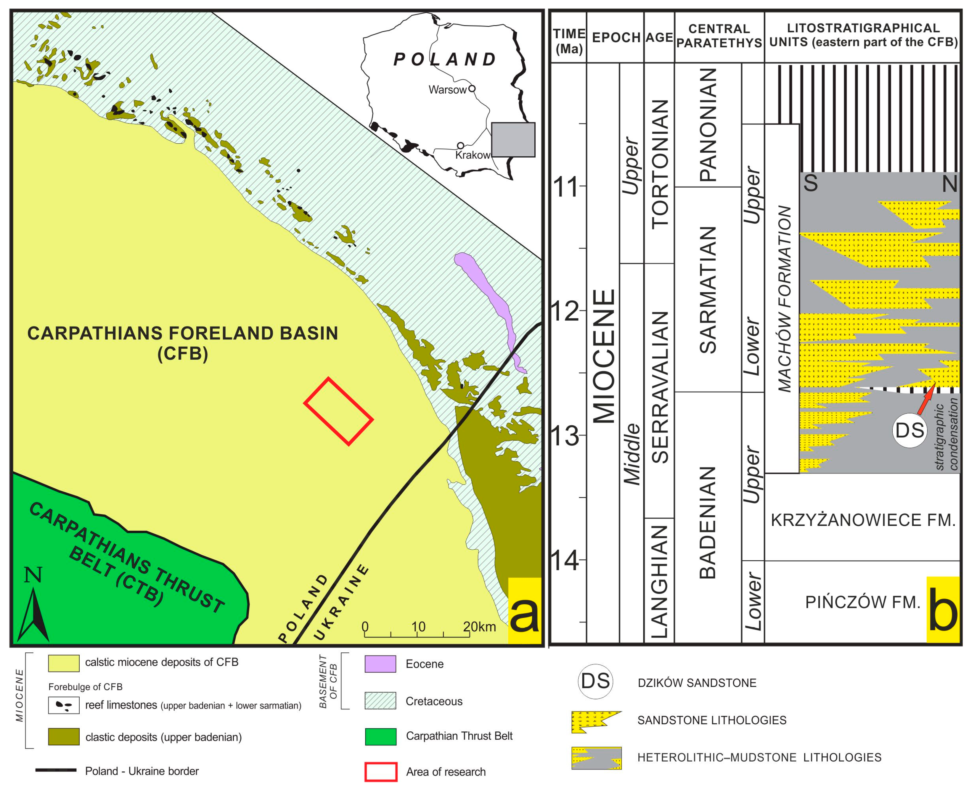
Figure 1. General characteristics of the research area: (a)—location of the study region on the map of the eastern part of the Carpathian Foredeep (after Dziadzio et al. [2]); (b)—Stratigraphy of Miocene deposits in the eastern part of the CFB (after Dziadzio et al. [2] and Porębski and Warchoł [12].
Energies 18 04521 g001
Figure 2. Workflow for defining gas-saturated zones.
Energies 18 04521 g002
Figure 3. The results of interpretation in well DZ-13 calibrated with laboratory data: NMR, PHI, PERM, and Carbonate volume. Dots visible in tracks 5–7 represent laboratory-measured porosity, permeability, and carbonate content. Dots in track 9 represent laboratory-measured irreducible water saturation.
Energies 18 04521 g003
Figure 4. The results of lithology interpretation calibrated with XRD data in well Z-1. Black dots visible in tracks 3–5 represent, respectively, the laboratory-measured values of clay volume, carbonate content, and quartz volume.
Energies 18 04521 g004
Figure 5. (A) Well log profiles and lithology with well test results and modified test results for impermeable zones in well Dz-20; (B) Well log profiles and lithology with well test results and modified test results for impermeable zones in well U-3. Description of data on each track: (1) Measured Depth; (2) GR (natural gamma-ray log), used for lithological identification; (3) NPHI (neutron porosity), DT (compressional slowness), and RHOB (bulk density); (4) RT (deep resistivity) and RX0 (shallow resistivity); (5) lithology; (6) the results of well tests (perforation); (7) adjusted well test results for impermeable zones.
Energies 18 04521 g005
Figure 6. The results of petrophysical data interpretation and machine learning-based classification of PETRO FACIES and RESERVOIR FACIES. The tracks are as follows: (1) depth (measured depth); (2) CALI (caliper log) and BS (nominal borehole diameter); (3) GR (natural gamma-ray log), used for lithological identification; (4) NPHI (neutron porosity), DT (compressional slowness), and RHOB (bulk density); (5) RT (deep resistivity) and RX0 (shallow resistivity); (6) VCL (clay volume); (7) PHI (core-calibrated porosity from MICP), PHIE (effective porosity), and PHIT (total porosity); (8) PERM (permeability); (9) lithology; (10) saturation analysis, including SWIRR (irreducible water saturation) and SW (water saturation); (11) perforation results; (12) RESERVOIR FACIES: dark blue—HWS; green—HWGS; yellow—HGS; gray—HNF; blue—BSWGS; pink—BSGS; (13) PETRO FACIES: RT 1—sandstones (yellow); RT-2—sandstone dominated heterolithes (orange); RT 3—mudstone-dominated heterolithes; RT 4—claystones and mudstones; and (14) stratigraphy.
Energies 18 04521 g006
Figure 7. (a) Inline 541 cross-section (A-A’) of the 3D seismic cube image with nearby boreholes: C-6, U-22, Dz-15, and D-1; (b) position of the A-A’ section against the 3D seismic cube range background.
Energies 18 04521 g007
Figure 8. Example of spatial visualization of the seismo-geological model. This surface represents the basal part of the Lower Sarmatian deposits, which include, among others, platform-derived Dzików sandstones. The yellow arrow marks the location of the Dzików sandstones (DS) on the RMS attribute map (DS—blue).
Energies 18 04521 g008
Figure 9. Spatial visualization of clay content: (a) N-S cross-section passing through the Dzików area. A characteristic depositional sequence of Dzików sandstones is visible in the basal part of the model; (b) NE-SW cross-section showing the varied morphology of sediments in the basal part of the model; (c) histogram of clay content value distribution.
Energies 18 04521 g009
Figure 10. Spatial visualization of effective porosity: (a) N-S cross-section passing through the Dzików area. A characteristic depositional sequence of Dzików sandstones is visible in the basal part of the model with high porosity values reaching up to 30% in some areas; (b) NE-SW cross-section showing the varied morphology of sediments in the basal part of the model; (c) histogram of effective porosity value distribution.
Energies 18 04521 g010
Figure 11. Correlation matrix for seismic attributes and reservoir parameters. High correlation features were grouped using hierarchical clustering and the Lance–Williams divergence update formula with Ward’s method.
Energies 18 04521 g011
Figure 12. Variable importance in the RF model RESERVOIR FACIES prediction in well logs.
Energies 18 04521 g012
Figure 13. Variable importance in the RF model PETRO FACIES prediction in the 3D model.
Energies 18 04521 g013
Figure 14. Variable importance in the RF model FLOW_TYPE prediction in the 3D model.
Energies 18 04521 g014
Figure 15. (A) Gas-saturated PETRO FACIES in sandstones (class 6); (B) gas-saturated SISMO FACIES in sandstones (class 6).
Energies 18 04521 g015
Figure 16. Analysis for the N-1 borehole (white dotted circle): (a) result of spectral decomposition with visible course of seismic profile from panel (b) (withe line); (b) seismic profile with visible position of seismic horizon presented in panels (a,c,e) (white arrow and line) and position of the N-1 borehole (red vertical line); (c) result of the SEISMO FACIES model; (d) profile (analogous position as in (b,f)) representing the result of the SEISMO FACIES model; (e) result of the PETRO FACIES model; (f)—profile (analogous position as in (b,d)) representing the result of the PETRO FACIES model.
Energies 18 04521 g016
Figure 17. Analysis of the Dzików region (white dotted circle): (a) result of spectral decomposition with visible course of seismic profile from panel (b) (white line); (b) seismic profile with visible position of seismic horizon presented in panels (a,c,e) (white arrow and line) and position of U-14 (left) and Dz-13 (right) boreholes (silting curve for each borehole); (c) result of SEISMO FACIES model; (d) profile (analogous position as in (b,f)) representing result of SEISMO FACIES model; (e) result of PETRO FACIES; (f) profile (analogous position to that in (b,d)) representing result of PETRO FACIES model.
Energies 18 04521 g017
Table 1. Data availability of well log data and laboratory data (number of samples) in 28 wells selected for analyses.
Laboratory Data
Well NameAvailable LogsPHIPERMXRDNMR
C-6CALI, BS, GR, NPHI, DT, RX0, RT%mD%%
DA-1CALI, BS, GR, NPHI, RX0, RT
DA-2CALI, BS, GR, NPHI, RX0, RT3
DS-2CALI, BS, GR, NPHI, RX0, RT446 10
D-12CALI, BS, GR, NPHI, DT, RX0, RT1414 14
D-13CALI, BS, GR, NPHI, DT, RX0, RT1919 19
D-15CALI, BS, GR, NPHI, RHOB, DT, RX0, RT1313 13
D-16CALI, BS, GR, NPHI, RHOB, DT, RX0, RT5
D-17CALI, BS, GR, NPHI, DT, RHOB, RX0,RT2622
D-18CALI, BS, GR, NPHI, DT, RHOB, RX0,RT31
D-19CALI, BS, GR, NPHI, DT, RX0, RT1713
D-20CALI, BS, GR, NPHI, DT, RX0, RT 5
D-21CALI, BS, GR, NPHI, DT, RHOB, RX0, RT12
D-24 *CALI, BS, GR, NPHI, DT, RHOB, RX0, RT
L-3CALI, BS, GR, NPHI, RX0, RT
N-1 *CALI, BS, GR, NPHI, DT, RHOB, RX0, RT89189
O-1CALI, BS, GR, NPHI, DT, RHOB, RX0, RT
SW-1CALI, BS, GR, NPHI, DT, RHOB, RX0, RT
U-3CALI, BS, GR, NPHI, RX0, RT
U-4CALI, BS, GR, NPHI, RX0, RT
U-12CALI, BS, GR, NPHI, RX0, RT
U-14CALI, BS, GR, NPHI, RX0, RT
U-19CALI, BS, GR, NPHI, RX0, RT
U-22CALI, BS, GR, NPHI, RX0, RT75
U-25CALI, BS, GR, NPHI, RX0, RT42
WC-1CALI, BS, GR, NPHI, DT, RHOB, RX0, RT
Z-1CALI, BS, GR, NPHI, DT, RHOB, RX0, RT 8
Z-2CALI, BS, GR, NPHI, DT, RHOB, RX0, RT
* Blind well.
Table 2. Description of models used in the study, with a list of variables, pre-processing, and tuning strategy.
MethodTarget ClassesInput VariablesPre-Processing StepsTuning StrategyVerificationComments
K-meansPETRO FACIES (RT1–RT4)PHIE, PERM, VCL, VCARBScaling and centering (step_normalize)--Large datasets (~100,000 observations)
Random ForestRESERVOIR FACIES in well logs (HWS, HWGS, HGS, HNCG, HNF, BSWGS, BSGS)DEPTH, PERM, NPHI, PHI, PHIE, PHIT, RT, SW, SWIRR, VCARB, VCL, VQRTZ, PETRO FACIESstep_dummy (PETRO FACIES), step_normalize, step_smote (RESERVOIR FACIES)Default: mtry = √(num predictors), trees = 500, min_n = 1Train/test split (80/20%)-
Random ForestPETRO FACIES in 3D seismic (RT1–RT4, plus RT5)AMP, SEISMIC_PHASE, RAI, SEISMIC_VARIANCE, AMPLITUDE_CONTRAST, INST_BANDWIDTH, LOCAL_FLATNESS, CHAOS, RMS, REFL_INT, ENV, SWEET, INSTANT_QUALITY, FREQUENCY, D1, D2, PHIE, K, VCLstep_normalize (all_numeric), step_smote (PETRO FACIES)RACES ANOVA (200 models, 20 combinations), mtry = 6, trees = 1000, min_n = 35Validation via bootstrapping (200 subsets), tested on 2 blind wellsLimited observations after upscaling to seismic grid
Random ForestRESERVOIR FACIES in 3D seismic (HWS, HWGS, HGS, HNCG, HNF, BSWGS, BSGS)Same as above plus PETRO FACIESstep_dummy (PETRO FACIES), step_normalize (all_numeric), step_smote (RESERVOIR FACIES)RACES ANOVA (200 models, 20 combinations), mtry = 9, trees = 1000, min_n = 11Validation via bootstrapping (200 subsets), tested on 2 blind wellsLimited observations after upscaling to seismic grid
K-meansSEISMO FACIES (1–12, plus 13)RAI, SWEET, RMS, INST_QUALITY, INST_BANDWIDTH, CHAOSYeo–Johnson transformation, scaling and centering (step_normalize)--Large seismic datasets (~10 mln observations)
Table 3. Metrics for the RESERVOIR FACIES prediction in well logs for testing datasets.
ClassPrecisionRecallF1 Score
HNF0.920.910.92
BSGS0.920.970.95
HGS0.950.900.92
HNCG0.600.800.69
HWS0.990.990.99
HWGS0.990.990.99
BSWGS1.001.001.00
Table 4. Metrics for the PETRO FACIES prediction in 3D seismic for validation datasets after analyzing 200 models (bootstrapping).
ClassPrecision (Mean)SDRecall (Mean)SDF1 Score (Mean)SD
RT10.700.160.650.180.650.13
RT20.820.040.880.030.850.02
RT30.820.020.780.020.800.01
RT40.780.020.800.020.790.01
Table 5. Metrics for the RESERVOIR FACIES prediction in 3D seismic for validation datasets after analyzing 200 models (bootstrapping).
ClassPrecision (Mean)SDRecall (Mean)SDF1 Score (Mean)SD
BSGS0.110.240.050.140.080.15
BSWGS0.810.090.810.070.810.06
HGS0.400.140.070.030.120.04
HNCG0.090.280.000.020.030.07
HNF0.820.020.840.020.830.01
HWGS0.700.020.780.030.740.02
HWS0.550.030.680.040.600.02
Disclaimer/Publisher’s Note: The statements, opinions and data contained in all publications are solely those of the individual author(s) and contributor(s) and not of MDPI and/or the editor(s). MDPI and/or the editor(s) disclaim responsibility for any injury to people or property resulting from any ideas, methods, instructions or products referred to in the content.