1. Introduction
Our society is highly dependent on the supply of electric energy. Its use is intense in domestic, commercial, and industrial environments. One of the key points of a high-quality electric power service is related to its continuity. The technical and economic consequences of interruptions in the electric energy service can be disastrous. Severe disturbances that lead to blackouts result in huge financial losses, and their restoration processes take considerable time. As an example, the US/Canada 2003 blackout led to an approximate USD 8.6 billion impact on the economy, and its restoration took up to 48 h [
1]. Since blackouts are the consequences of voltage instabilities in power systems, appropriate monitoring and assessment of voltage stability conditions is of vital importance. A secure operation from the voltage stability standpoint can be guaranteed by maintaining an appropriate voltage stability margin (VSM), or loading margin, especially during heavy load periods. Therefore, a power system is secure from the voltage stability standpoint if it can withstand a certain load increase while keeping an appropriate voltage profile.
Even though several aspects of the voltage stability problem have been known for decades, the assessment of the voltage stability condition of power systems during real-time operation is still a challenge, since it demands efficient, robust, and fast methods to compute it.
The power stability problem is classified into several categories, and appropriate models and analysis methods are used in each case [
2]. In this paper, since the voltage stability problem will be tackled, steady-state models associated with long-term disturbances will be adopted.
The voltage stability phenomenon has been studied for a long time, and the available literature is vast. In this paper, we opted to cite just a few references, in order (a) to show examples of the different approaches that have been proposed in the last decades; and (b) to support the methods proposed here.
A careful review of the literature suggests that the voltage stability analysis approaches specifically proposed to deal with long-term phenomena can be generally classified as model- or measurement-based [
3].
Several model-based analysis models can be found in the literature, such as
(1) the continuation methods [
4],
(2) the optimal power flow methods [
5],
(3) the direct methods [
6], and
(4) the power flow methods [
7]. Most of these methods include detailed models for the systems, such as equipment bounds and control variables. In general, however, they may be computationally expensive, which is an important disadvantage when it comes to real-time operation analyses.
Most measurement-based methods are based on the so-called voltage stability indices (VSI) [
8,
9,
10,
11,
12,
13]. More recently, the wide use of synchronized phasor measurement has led to the proposal of new voltage stability indices. Most of these indices are based on Thevenin equivalent circuits [
3,
4,
11]. One of the important advantages of VSIs is the computational efficiency of their computations, which is highly convenient for real-time operation analyses. On the other hand, the utilization of VSIs may present some disadvantages. Firstly, even though VSIs can be efficiently used to compare the voltage stability conditions of different power systems, their values cannot be directly related to their VSMs. Several VSIs are defined to range from zero (for example, corresponding to no load conditions) to one (for example, corresponding to the maximum loading point). A particular VSI value of, say, 0.8, is not at all related to a voltage stability margin given in power (MVA, MW, or MVAr) [
14]. Secondly, the equations for the calculation of VSIs do not allow the inclusion of power systems’ physical constraints, such as generators’ reactive power bounds. An attempt to include such bounds was made in [
11], where an index based on sensitivities was proposed to predict when the generators’ reactive power bounds would have been reached. It is a well-known fact that VSIs may experience abrupt changes when generators reach their respective reactive power limits. According to [
11], this change can be as low as 0.01 or as high as 0.5, depending on the importance of the generator for the power system. Finally, relating a certain change in a VSI to a change in the VSM is not an easy task.
It is important to mention that power systems have been experiencing important changes related to the energy transition, especially by replacing fossil-based generation with cleaner renewable generation, particularly wind and solar. The increasing penetration of intermittent non-dispatchable types of generation will influence systems’ loadings and their voltage stability conditions [
15,
16,
17].
The proposed approaches found in the literature for assessing the voltage stability condition of power systems are usually either (a) accurate and computationally burdensome, or (b) less accurate and computationally efficient, which is a conflicting situation. So, the main objective of this research work is to propose a method that fulfills both the requirements related to accuracy and computational burden.
In this paper, a new, accurate, and computationally efficient method for computing the voltage stability margins of power systems is proposed for real-time operation applications. The proposed method incorporates the qualities of both model-based and measurement-based models, leading to an efficient combination of three ideas already present in the literature, as described below.
Table 1 summarizes and clarifies the above discussion.
Both PM1 and PM2 will be described in detail, and the computer simulations will show that they are robust and computationally very fast for determining the MLP and the VSM of power systems, making them appropriate tools to be used in real-time power system operation.
M1, M2, and M3, as well as PM1 and PM2, will be described in the following sections. Then, results from computer simulations will be shown and discussed to support the claims made above.
2. Theoretical Framework
The theoretical background necessary for the appropriate understanding of the proposed method will be presented and discussed in this section.
2.1. Second-Order Power Flow with Step Size Optimization (PFSSO) [22,23]
Power systems operating in steady-state conditions can be represented by the following set of algebraic nonlinear equations.
Array corresponds to the system’s state variables, namely voltage magnitudes () and phase angles (). Scalar is the loading factor. In this paper, multiplies all bus power injections, so power factors are kept constant.
Equation (1) can be rewritten as
Arrays and correspond to the mismatches of real and reactive powers, respectively. and are the arrays of calculated and scheduled nodal real powers, respectively. depends on the state variables, whereas is a function of the loading factor. is the array of base case real power injections. Of course, similar definitions hold for the reactive power quantities.
The power flow iterative process considers the reactive power generation limits of PV buses. Whenever the reactive power limit is violated at some bus, its type is switched from PV (generation bus) to PQ (load bus). These new PQ buses can be switched back to PV in further iterations, depending on the voltage magnitude variation and the respective violated limit (upper or lower). This feature is not explicitly shown in (1) and (2), but its computational implementation is straightforward.
The representation of additional characteristics of loads and generators other than reactive power limits, such as rates of change, can be implemented by modifying (1) and (2) [
4]. This flexibility can be particularly useful when the network contains non-dispatchable generation sources such as wind and solar.
The conventional iteration-based power flow methods may not converge or may diverge for the so-called ill-conditioned power systems [
7,
22,
23]. These numerical difficulties may occur even if the system operates normally in a stable equilibrium point.
PFSSO is an efficient, non-divergent, and robust power flow method [
24]. Originally, the bus voltages were represented in rectangular coordinates. An alternative version of this method was proposed in [
22,
23], where voltages were represented in polar coordinates. An improved power flow method with voltages in polar coordinates, which resulted in a more robust method than the previous ones, was proposed in [
25].
The conventional Newton’s method applied to power systems consists of obtaining the state variables starting from an initial guess through steps . The main idea of PFSSO is to adjust the step size to avoid numerical problems, basically related to the ill-conditioning of the nonlinear algebraic set of power flow equations. This adjustment is included in Newton’s method by multiplier , which considers first- and second-order information from the Taylor series expansion of (1), as will be described ahead.
At iteration
, the state variable array
is obtained by
where
corresponds to the Jacobian matrix of (1), and
μ(r) is the optimal multiplier that adjusts Newton’s step size.
μ(r) is computed by minimizing the quadratic function
based on the nodal power mismatches, as
Ω
g is the set of power flow equations
that contains the real and reactive power equations of load buses (PQ) and the real power equations of generation (PV) buses.
is an array that contains the expansion of
in the Taylor series by retaining only the first- and second-order terms [
23]:
where
T(
x) is an array that contains the second-order terms of
, given by
By replacing (5) in (4), one obtains a fourth-degree polynomial. Its local minimum is found by imposing
, which leads to a cubic equation whose unknown is
μ [
23]. The optimal multiplier is one of the roots of the cubic equation, and it is used in (3) to control Newton’s step size.
The main features of the optimal multiplier
are three-fold [
7,
22,
23].
(a) The computed optimal multipliers for well-conditioned systems are close to one. In these situations, PFSSO behaves similarly to the conventional Newton’s method.
(b) If the power system is ill-conditioned,
μ assumes values at each iteration to overcome numerical problems that could result in divergence or non-convergence. Eventually, PFSSO converges to the correct stable solution [
22,
23].
(c) Infeasible systems do not have a state variable array
that meets the power flow Equation (1). In this case,
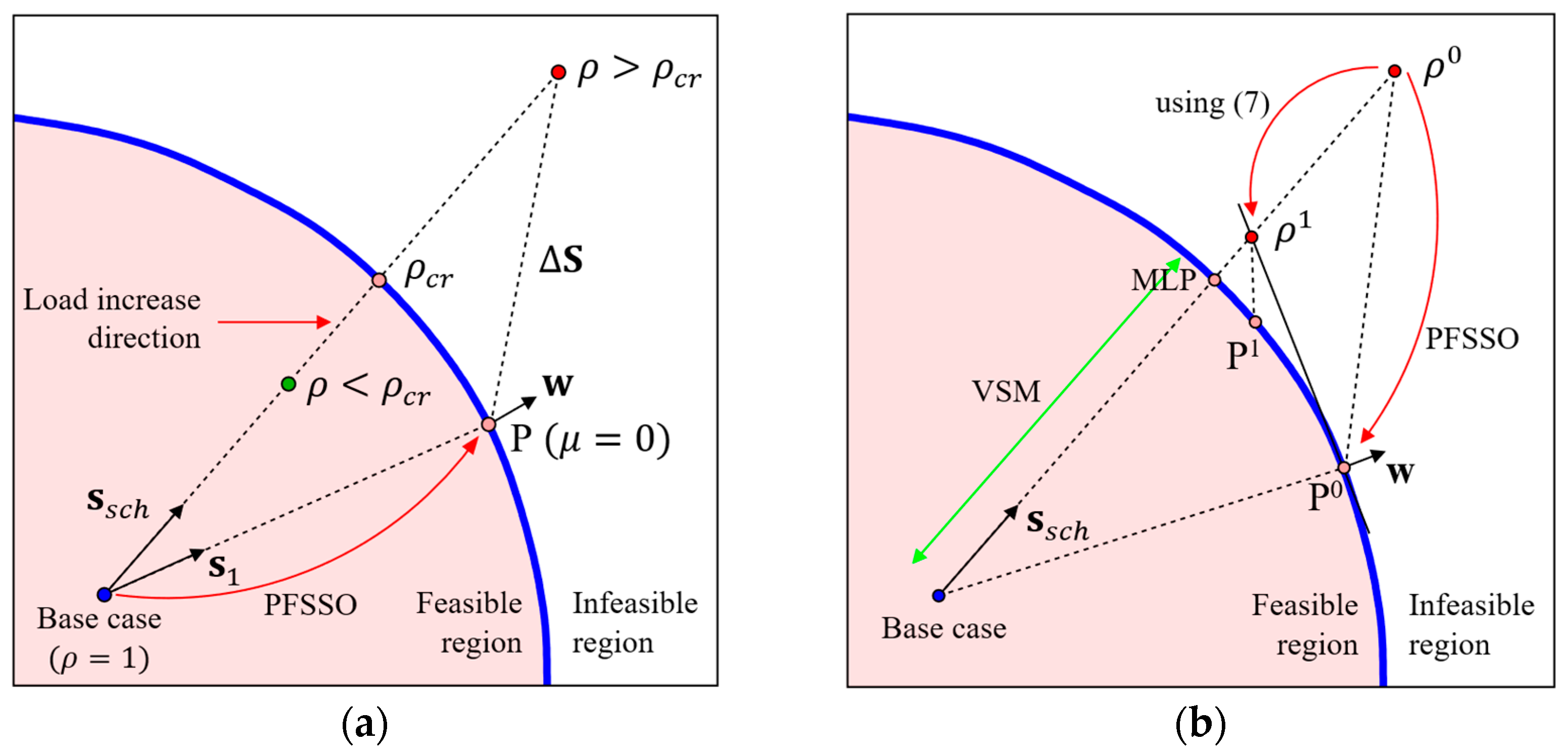
μ tends to zero during the iterative process, eventually reaching zero (or, in practice, a value smaller than a predefined threshold). Infeasibility may result from situations like contingencies or unexpected excessive loadings. When the optimal multiplier approaches zero, PFSSO converges to an operating point on the feasibility boundary in the load parameter space (as demonstrated in [
26] and illustrated in
Figure 1), while the conventional power flow would have failed. At this boundary point, the Jacobian matrix is singular. This property is very useful, since information regarding this point can be used in several power system studies, including voltage stability analysis. This feature will be explored ahead.
2.2. Computing the MLP Using PFSSO [7]
The basic principles for the computation of the MLP were proposed in [
7], based on the exceptional features of the PFSSO [
22,
23].
Figure 1a shows a simple representation of a two-dimensional load parameter space. Consider that the base case corresponds to (
). Loading factor
multiplies all elements of the scheduled power array as shown in (2), so that power factors remain constant. As
increases, the operating point is driven along the load direction
. The objective is to obtain the MLP, which corresponds to the loading factor
. While the load increases, that is,
is smaller than
, PFSSO converges to a feasible stable operating point. However, if an infeasible point is reached, that is,
, PFSSO converges to a point on the feasibility boundary
(point P), as shown in [
26], and
tends to zero. Note that point
is the MLP along the load increase direction
. Depending on the value of
, different MLPs on
are obtained by PFSSO. Also, array
is the left eigenvector related to the zero eigenvalue of the Jacobian matrix at
, and it is normal to the feasibility boundary
[
26].
Array
in
Figure 1a contains the power mismatches provided by PFSSO, and it corresponds to the distance between operating point
and scheduled point
in the parameter space.
According to [
7], the load correction
is calculated from
and
. Scalar
approximates the new estimate of the desired maximum loading point along
. The VSM is the distance between the MLP and the base case in parameter space.
A detailed procedure for computing the MLP is proposed and discussed in [
7]. For the sake of completeness, the main features of such a procedure will be highlighted here.
Figure 1b illustrates a two-dimensional load parameter space, like
Figure 1a. If an initial loading factor
is set up in the infeasible region, PFSSO converges to the operating point
on the boundary
. The new loading factor estimate
is given by:
The loading factor correction computed from (7) considers the power mismatches provided by PFSSO and the left eigenvector associated with the zero eigenvalue of the Jacobian matrix. The new loading factor estimate corresponds to an infeasible operating point, and running PFSSO leads to boundary point . The steps just described suggest an iterative procedure. Therefore, new loading factors are computed successively until the MLP along the desired load increase direction is achieved.
Note that the procedure described earlier starts with an infeasible loading factor . The steps described earlier, starting from an infeasible point, are only possible due to the special features of the non-divergent method PFSSO. Of course, running the conventional power flow methods would result in divergence, and no relevant information could have been retrieved to compute the MLP. Nonetheless, even though the procedure described above considered an infeasible loading factor as the initial point, the proposed methods can perform well in the case of feasible initial operating points. Note also that intermediate points , , and further operating points computed in the iterative process are located on the feasibility boundary . Therefore, it is reasonable to expect that some generators’ reactive power limits would have been reached at these points. Of course, PFSSO can handle this situation appropriately, and this is one of the advantages of the proposed methods.
Depending on the analysis being carried out, each utility can define an acceptable error in the value of the MLP (the difference between the computed MLP and the actual exact MLP). For example, an error of 5% could be acceptable and would not interfere with the necessary control actions to be taken.
According to [
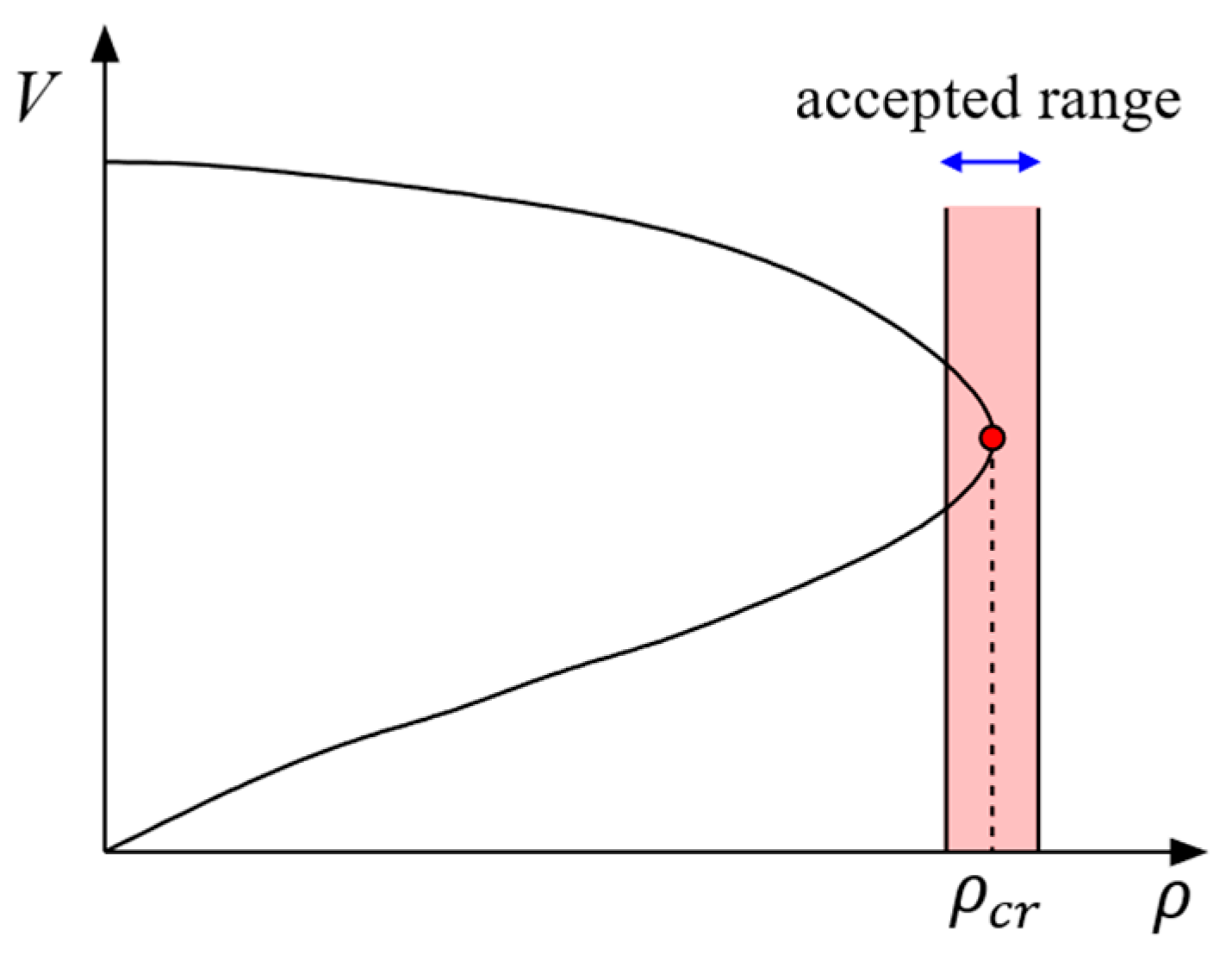
7], it is possible to include information about this acceptable error in the proposed methods. Suppose that an acceptable error of 5% is defined by a certain utility. Therefore, loading factors in the range
are acceptable for practical purposes. A PV curve, along with a graphical interpretation of the acceptable range, is shown in
Figure 2.
Consider that
% is an acceptable error range in the MLP. Consider also that scalar
is associated with the range of acceptable solutions, given by:
Method
M1 proposed in [
7] is described below.
- (1)
Set iteration counter . Set initial loading . It is usual, though not mandatory, to set large enough to establish an infeasible operating point.
- (2)
Run PFSSO for . If the operating point is infeasible (), continue; else, go to step (5).
- (3)
Obtain , where is computed by (7).
- (4)
Run PFSSO for . If the operating point is feasible, continue; else, go to step (6).
- (5)
Run PFSSO for . If the operating point is infeasible, the final solution is given by ; else, set (average of the most recent feasible and infeasible points). Increment the iteration counter and go to step (2).
- (6)
Run PFSSO for . If the operating point is feasible, the final solution is ; else, increment counter and go to step (3).
The simulation results shown in [
7] certify that
M1 is robust, efficient, and accurate.
Finally, M1 has some important features that are worth mentioning.
M1 is based on running PFSSO. Therefore, the inclusion of all controls and limits occurs naturally in the power flow formulation.
The simulation results shown in [
7] demonstrate that a more efficient iterative process occurs when the initial point is infeasible (
). In this case, the number of iterations and PFSSO runs are smaller. However, any initial loading factor
can be used, and
M1 can still provide accurate results.
The efficiency of the iterative process depends on the distance between the initial loading factor and the maximum loading factor .
2.3. Linear Voltage Stability Index [18]
Reference [
18] proposed a linear voltage stability index (VSI). The linearity of this VSI is very attractive, since it can be used directly to estimate the maximum loading point, and hence the voltage stability margin. Following the concept of other VSIs proposed in the literature, this linear index is derived from the Thévenin equivalent circuit, under the assumption of a multi-port network equivalent model [
18,
27], and it is computed for each bus of the network. The derivation of this index is shown in detail in [
18]; nonetheless, a brief description of its main features follows for the sake of clarity.
The multi-port network equivalent model of a power system can be given by:
is the system’s admittance matrix;
and
are the current injections and bus voltages, respectively. Subscripts
,
, and
correspond to generation, load, and zero-injection buses. According to (9), the load voltages are given by:
where
Considering that the matrix
remains constant as the load increases, the voltage at bus
is given by:
where
and
are, respectively, the numbers of load and generation buses.
and
are, respectively, the equivalent voltage and impedance related to bus
after applying Thevenin’s theorem. Assuming that
and
remain approximately constant as the load increases, the linear index associated with bus
is defined in [
18] as:
where
According to [
18], the voltage stability index for the entire system is defined as:
and the respective maximum real power is:
As an example,
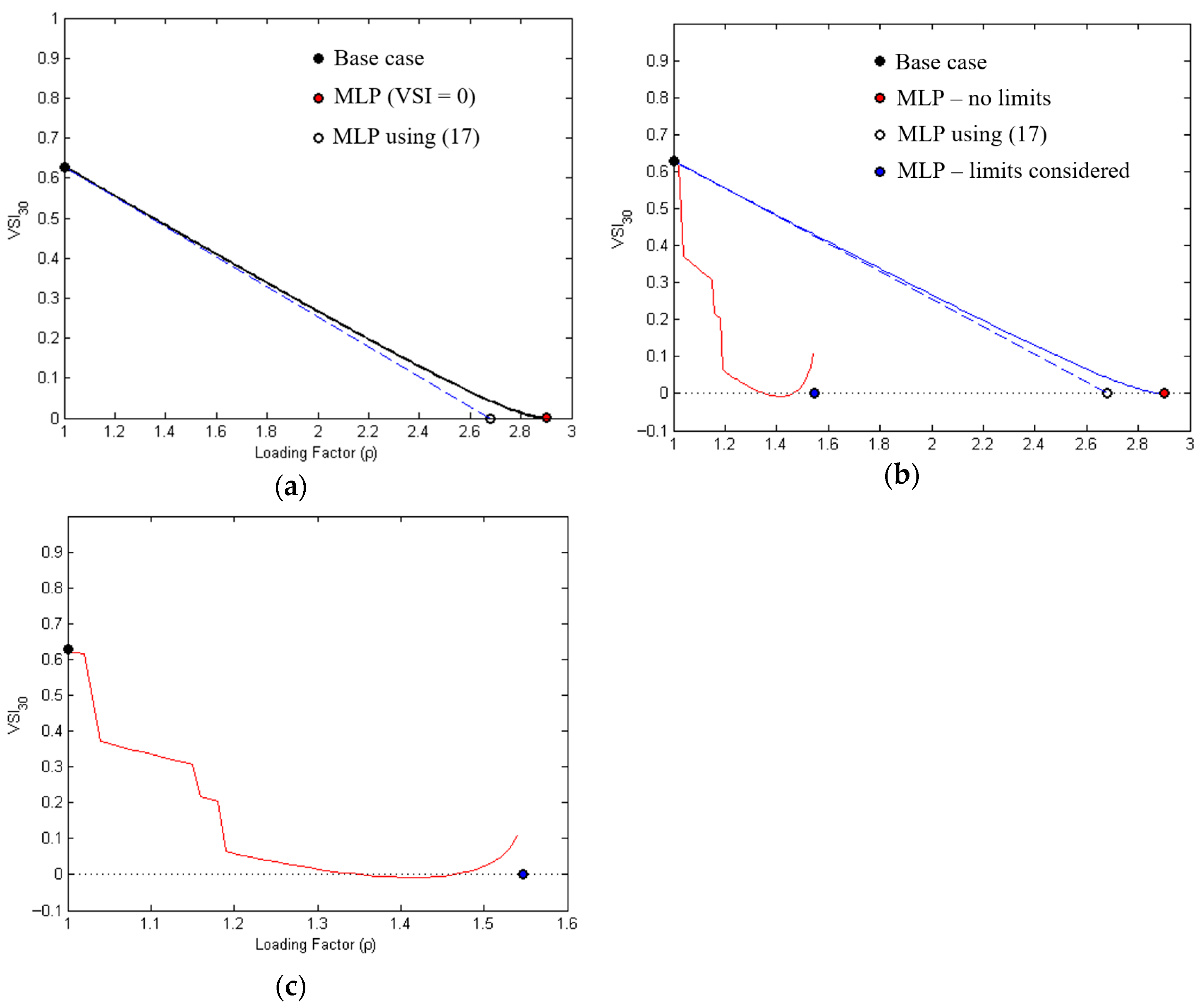
Figure 3a illustrates the evolution of the linear voltage stability index for bus 30 of the IEEE 30-bus system [
28]. In this case, generators’ reactive power limits were not considered. After increasing
from the base case (
) up to a point for which the conventional power flow did not converge, and calculating the VSI from (14) and (15), the MLP was estimated as
.
Figure 3a also shows that the actual behavior of the index is not linear. From (17), the computed MLP is
. Therefore, there is an error of 7.4% with respect to the actual MLP.
Note that the MLP computed by (17) does not consider the generators’ reactive power limits. On the other hand, the authors in [
18] stressed the importance of including the reactive limits of generators, since generator limitations significantly affect the MLP. Thus, neglecting such limits leads to considerable errors, which is not reasonable for practical purposes.
Figure 3b illustrates the evolution of VSI
30 when the generators’ reactive power limits are considered. The MLP in this case is
, which is significantly smaller than the one computed without reactive power limits.
Figure 3b shows that the index is piecewise linear. Discontinuities occur whenever some generator reaches its respective reactive power limit. Moreover, the VSI becomes nonlinear in the vicinity of the maximum loading point.
Figure 3c illustrates a detailed view of the evolution of VSI
30 considering generators’ reactive power limits. In [
18], the VSI is derived based on a linear model, so the actual nonlinear behavior due to the reactive power limits is not accounted for.
In this research work, a method referred to as M2 is proposed for obtaining the MLP based on VSI. The steps of M2 are as follows:
- (1)
Set loading factor (system’s base case).
- (2)
Compute the maximum loading factor using (17).
Some considerations regarding
M2 are as follows:
(a) the calculation of
is very fast, since (17) is based on a system of linear equations (9);
(b) the derivation described in [
18] (and briefly shown here for the sake of clarity) does not consider equipment controls and limits.
The idea is to use loading as an initial point for the proposed method PM1.
2.4. Sensitivity of Generators’ Reactive Powers with Respect to System’s Loading [19,20,21]
Consider the set of nonlinear algebraic power flow equations given by (1). They can be rewritten as:
A loading change
leads to a change in the system’s operating point
, as follows:
where
is an
array,
is the
Jacobian matrix,
is a scalar, and
is an
array of the sensitivities of the state variables with respect to the loading
.
is an
array given by:
A functional dependent variable
, such as the reactive power at a generation bus, is also dependent on the state variables
and the loading
, and can be represented by:
Changes in
due to changes in
can be estimated by their sensitivities as:
where
is an (
) array corresponding to the sensitivities of the reactive powers with respect to
, and
is an (
) array of derivatives of
with respect to state variables
[
21]. The matrix
can be obtained by:
where
is formed by elements of the Jacobian matrix. The net reactive power injected at the generation bus
is given by:
where
and
correspond to the generated and consumed (load) reactive powers, respectively. From (24),
Consider now an array
containing all reactive powers generated at each bus, defined as:
where the array
is of dimension (
). It has been observed that a loading change
leads to a state variable change
. In turn,
leads to a change in the reactive power injections. Therefore:
since
is constant and does not depend on
. Therefore, considering also (19), we obtain:
Matrix
is given by:
where
is an (
) matrix formed by elements of the Jacobian matrix.
The sensitivity factors allow the search for the smallest loading change such that a generation bus reaches its reactive power generation limit [
20]. This loading change is given approximately by [
19]:
where
if
, or
if
. The individual loading changes relating to all generators are computed by:
Then, the average loading
is computed by:
where
is the number of generators whose loadings
are less than the loading defined by the linear VSI
. Now, the average loading
obtained from the sensitivity analysis and the loading
obtained by the linear VSI can be combined to define the initial loading for the proposed method
PM2, as will be shown in the next section.
3. Proposed Methods
In this paper, the two proposed methods are referred to as
PM1 and
PM2. They are intended to take advantage of the strengths of
M1,
M2, and
M3, while also overcoming their occasional limitations. Furthermore,
M1 has been enhanced compared with [
7], enabling it to handle feasible operating points more efficiently throughout the iterative process.
The proposed method PM1 is described in Algorithm 1.
| Algorithm 1. PM1. |
| M2 (Section 2.3) |
- (1)
. - (2)
using (17). This point corresponds to an approximate MLP.
|
| M1 (improved) (Section 2.2) |
- (3)
. - (4)
and continue. - (5)
, and repeat step (5). - (6)
,, set and go to step (8). Otherwise, continue. - (7)
. If the converged point is infeasible, go to step (9). Otherwise, continue. - (8)
and go to step (4). - (9)
as the solution and stop.
|
Steps (1) and (2) correspond to method
M2 as described in
Section 2.3. The linear voltage stability index computed by (17) in step (2) provides an initial estimate of the maximum loading point, which serves as the starting point for
M1. Steps (3) to (9) correspond to
M1, as described in
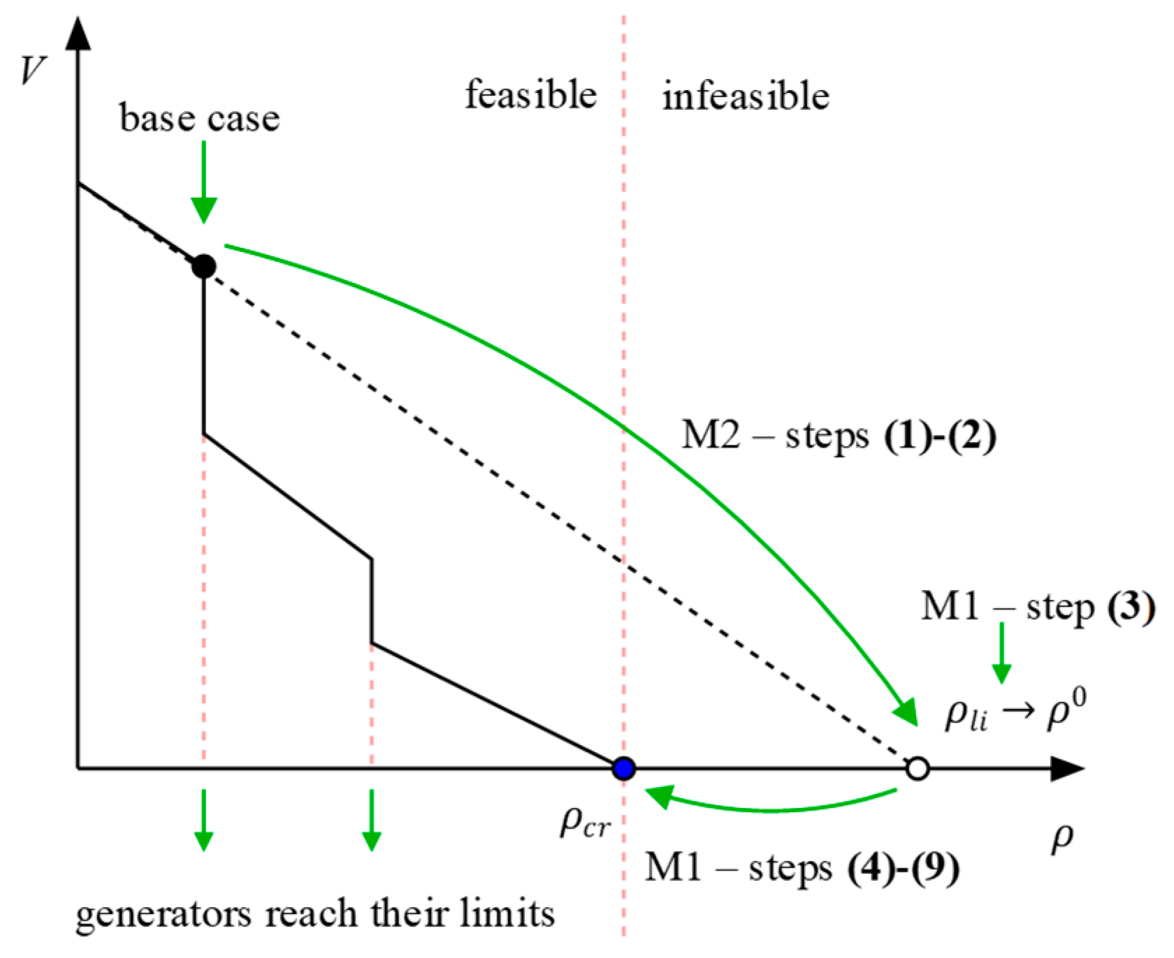
Section 2.2. Note that the first run of PFSSO in step (4) uses the loading estimated by the linear voltage stability index computed by (17). The iterative process yields the actual maximum loading point. The slight yet crucial modification introduced in step (3) furnishes an educated initial guess, which is infeasible for most systems, as will be demonstrated ahead. However, since this initial point is obtained via
M2, the value
from step (2) is expected to be close to the actual maximum loading point.
It is important to note that, in general, the Thevenin equivalent model inherently simplifies the network. Nevertheless, the proposed methods demonstrate sufficient robustness to refine the initial estimate and accurately determine the desired MLP, in accordance with the predefined acceptable error ε.
Figure 4 illustrates the steps of
PM1, where each point represents the algorithm presented above.
For some systems, the loading factor calculated in step (2) may be feasible. Regardless, M1 can effectively handle such cases, as demonstrated in steps (3)–(9). Furthermore, note that the computational effort required by PM1 (steps (1)–(9)) is directly related to the number of power flow runs needed for convergence.
The proposed method PM2 is described in Algorithm 2.
| Algorithm 2. PM2. |
| M2 (Section 2.3) |
- (1)
. - (2)
, corresponding to the MLP, using (17).
|
| M3 (Section 2.4) |
- (3)
. - (4)
. - (5)
as in (32).
|
| M1 (improved) (Section 2.2) |
- (6)
. - (7)
and continue. - (8)
, and repeat step (8). - (9)
,, set and go to step (11). Otherwise, continue. - (10)
. If the converged point is infeasible, go to step (12). Otherwise, continue. - (11)
, and go to (7). - (12)
is the solution. Stop.
|
In PM2, the initial estimate computed using the linear VSI (step (2)) is used as a cap value for the estimates obtained through sensitivity analysis (step (4)). The average of these estimates results in the first operating point (step (5)), which will be used by PFSSO in step (7). PM2 was developed to be even more robust than PM1, since a better initial loading factor is computed for M1. Consequently, fewer power flow computations will be necessary to achieve the actual maximum loading point.
Although the proposed methods in this manuscript are based on (2)—that is, the power system operating state is changed by assuming a constant power factor—they can be adapted to different formulations, such as the one used in [
4], where different patterns of load and generation increases are possible.
4. Simulation Results
In this section, the computer simulation results are presented, ranging from small benchmarks to large realistic power systems. The small systems used are the standard IEEE 14-, 30-, 57-, 118-, and 300-bus systems whose data were obtained from [
28]. The data for the large systems were also provided by [
28], and they “represent the size and complexity of part of the European high-voltage transmission network.” [
28]. The power flow runs for computing the linear index
and the sensitivity-based index
were carried out with version 6.0 of Matpower [
28], applying a threshold of 0.01 MW/MVAr for power mismatches. For PFSSO, a threshold of 0.001 was adopted for computing the optimal multiplier
, while 0.1 was considered the threshold for the minimum nonzero step size. In other words, optimal multipliers less than 0.1 were treated as zero.
4.1. Proposed Method PM1
4.1.1. IEEE Test Systems
The standard IEEE 14-, 30-, 57-, 118-, and 300-bus systems are used in the computer simulations. Method
M1 requires defining the parameter
, which determines the acceptable error in calculating the VSM.
Table 2 and
Table 3 present the simulation results considering acceptable errors of
and
, respectively.
In
Table 2 and
Table 3,
represents the actual maximum loading factor obtained through successive runs of the conventional power flow with incrementally increasing loading, until divergence occurs. The reactive power limits of generators are taken into account.
serves as a reference value for further comparisons.
is the maximum loading factor computed by
M2—steps
(1)–
(2) of
PM1—and is used as the initial value for
M1—steps
(3)–
(9) of
PM.
denotes the maximum loading computed by
PM1. #Iterations refers to the number of iterations required for
PM1 to converge within the acceptable error
, and #PFSSO indicates the number of power flow runs using second-order step size optimization. In the case of the IEEE 57-bus system, note that
—meaning the initial guess for
M1 is a feasible operating point. As previously mentioned, this has no impact on the convergence of
PM1, underscoring its robustness.
To clarify the process of calculating the initial loading factor estimate
(which is equal to
), consider the IEEE 14-bus system. The voltage stability indices (VSIs) computed using (15), as well as the initial loading estimate
computed using (17) for the load buses, are presented in
Table 4.
According to
Table 4, the smallest VSI—and consequently, the smallest loading factor—corresponds to bus 14. The corresponding
is assumed as
in
Table 2 and
Table 3. The evolution of the loading factor
and the number of power flow runs for the IEEE 14-bus system are depicted in
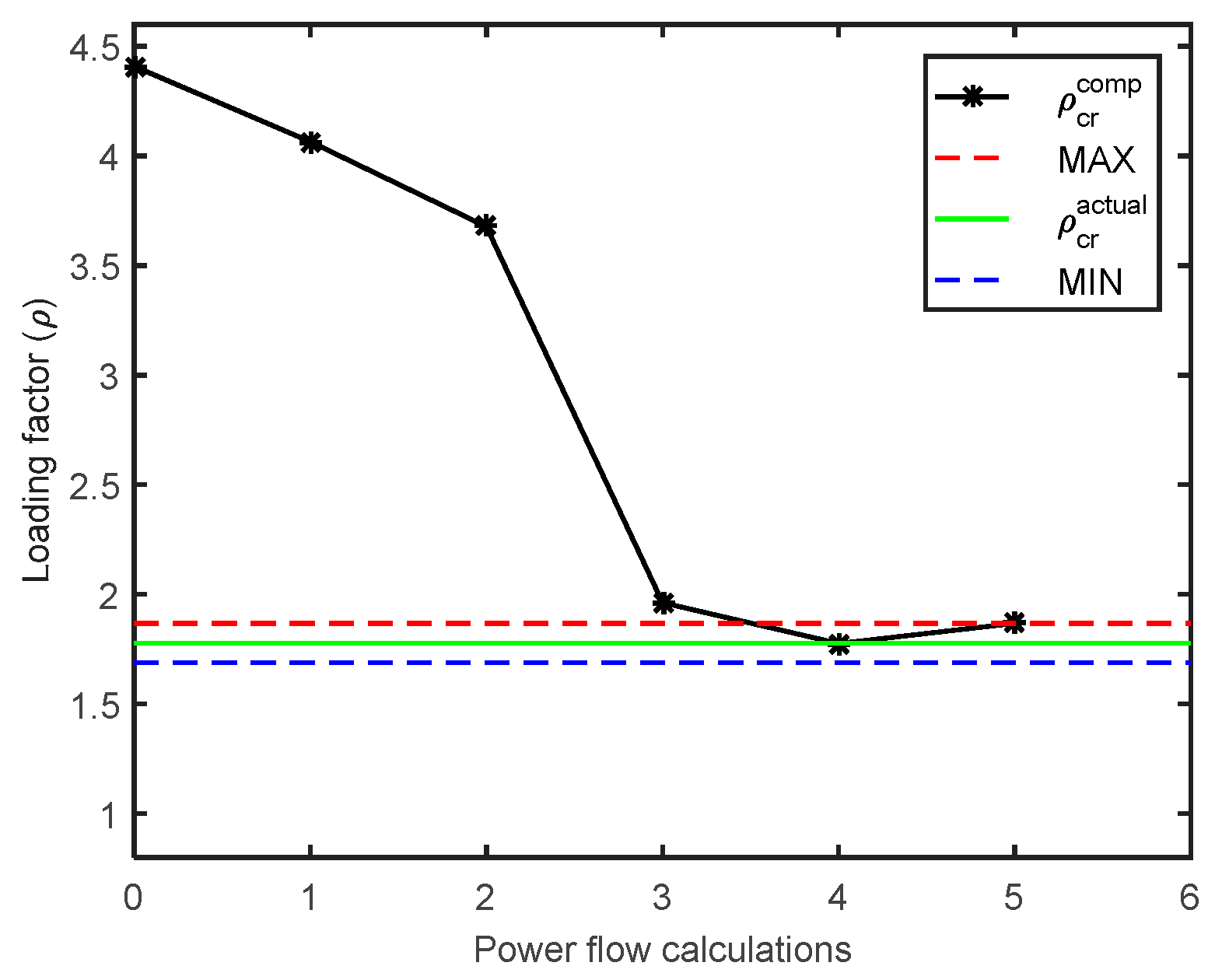
Figure 5. The dashed lines represent the range of acceptable solutions, in this case considering
.
PM1 converges after a few power flow executions.
4.1.2. Large Systems
The results provided by
PM1 for larger realistic systems [
28] are presented in
Table 5. The number of iterations and power flow runs required for
PM1 to converge are small, consistent with those obtained for the IEEE systems.
In
Table 5, the maximum loading computed from
M2 (
) falls outside the acceptable error range (
). The main reasons for this are as follows: (a) the linear nature of the voltage stability index, and (b) the omission of the generator reactive power limits (see
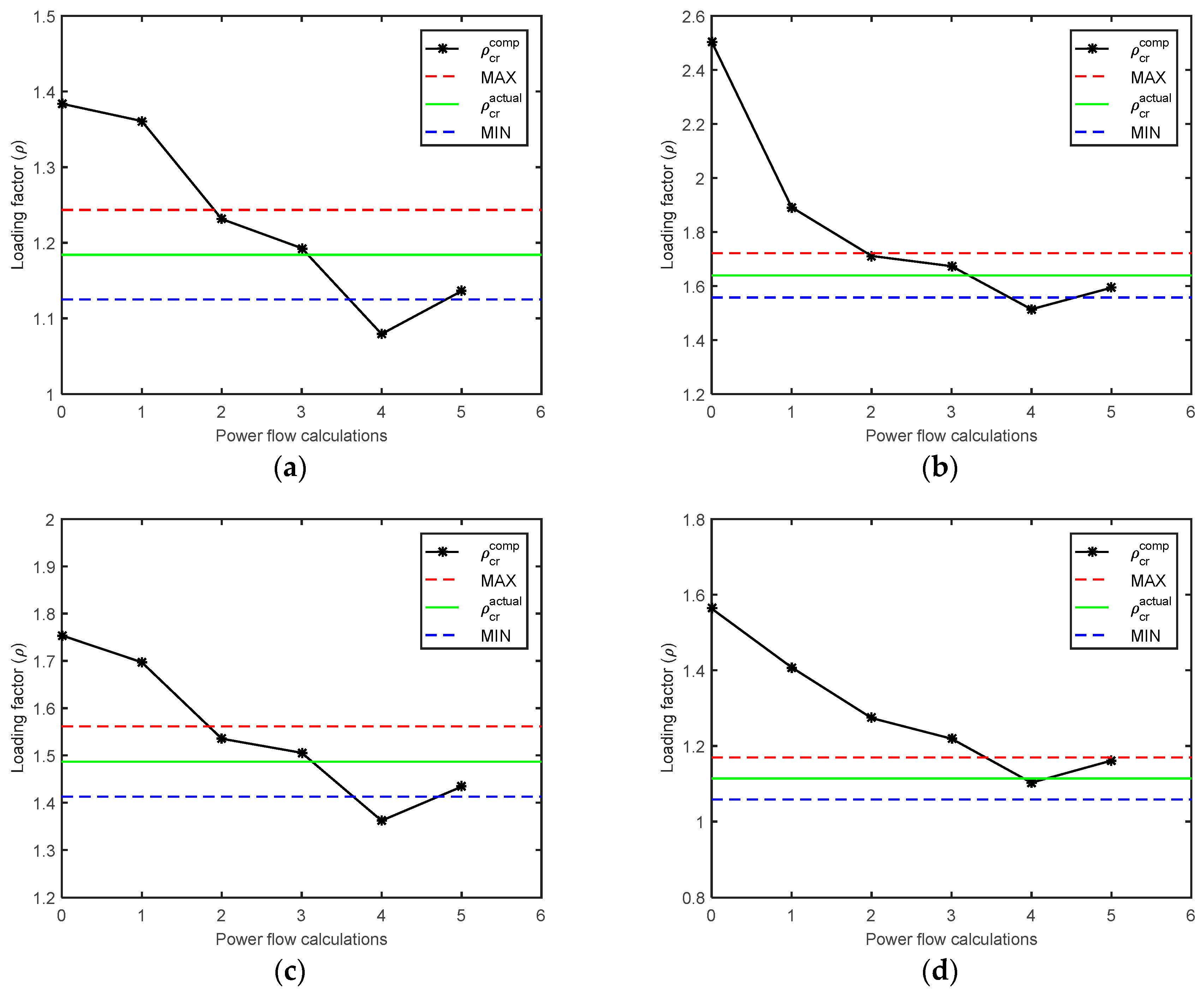
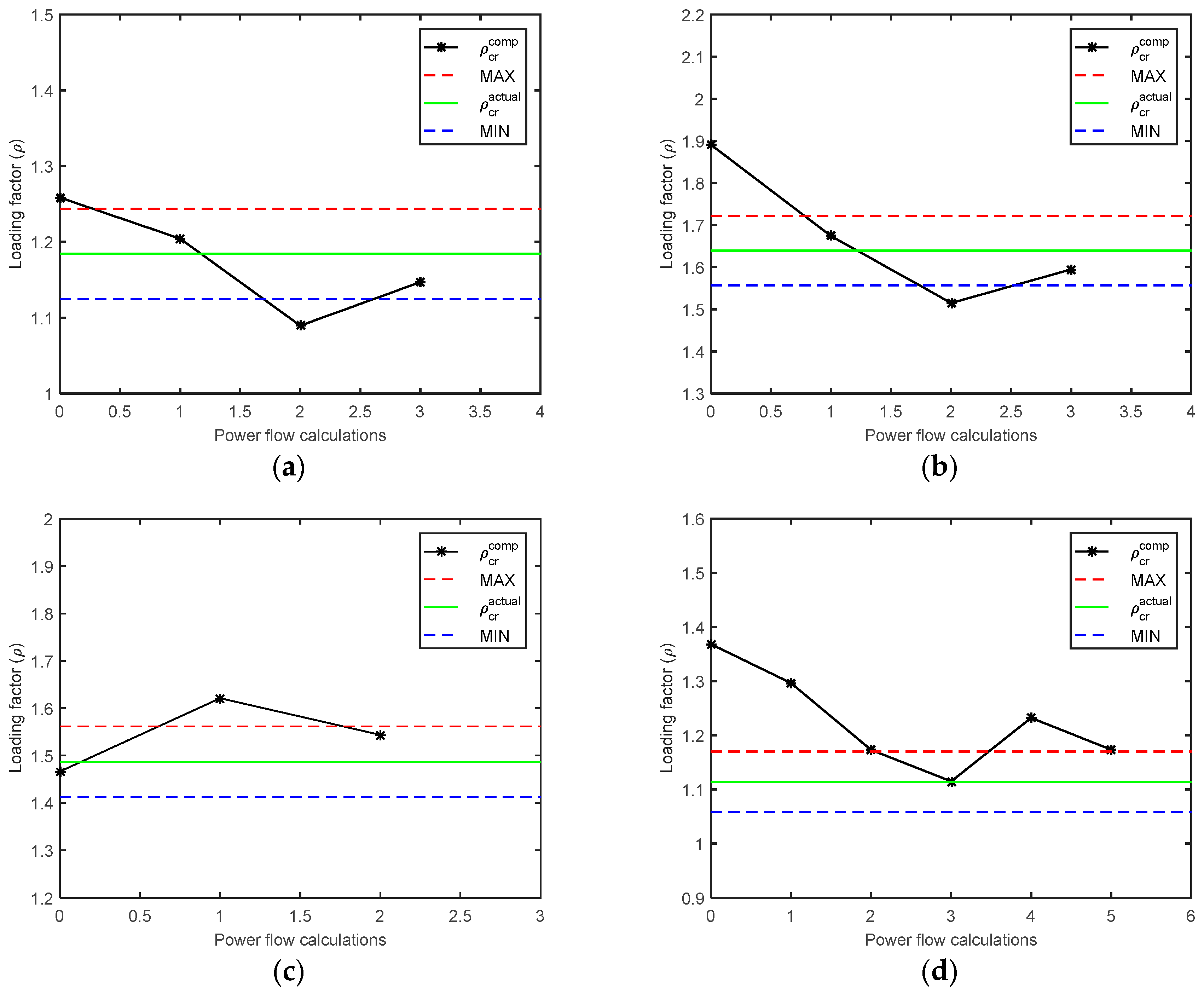
Figure 4). The evolution of the loading factor as a function of the number of power flow runs for the systems in
Table 5 is illustrated in
Figure 6, considering an acceptable error
at the final maximum loading point.
Using the linear voltage stability index from [
18] to estimate the maximum loading point (
M1) is computationally very efficient. However, system limits and control mechanisms cannot be accounted for, which leads to significant inaccuracies. Employing the maximum loading factor derived from the linear index as an initial estimate for the iterative method
PM1 results in a highly efficient iterative process. The number of iterations required for convergence, as well as the number of power flow runs, decreases significantly.
PM1’s performance benefits from this strategy. The maximum loading point calculated by
M1 for different initial values of
is displayed in
Table 6.
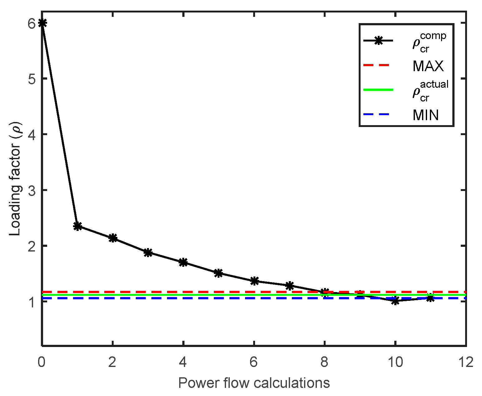
Figure 7 illustrates the behavior of the maximum loading factor as a function of the number of power flow runs for an initial loading of
.
Table 6 shows that method
M1 can compute both the maximum loading and the voltage stability margin within the predefined acceptable error range (
), regardless of the initial guess. This behavior was also demonstrated in [
7]. The number of iterations required for convergence is related to the initial guess—a value closer to the actual VSM results in fewer iterations.
Nonetheless,
Table 6 also shows that method
M1 performs much more efficiently when an informed initial guess is used (provided by
M2), resulting in a significantly smaller number of required power flow runs. Therefore, integrating
M1 with
M2—resulting in
PM1—leads to substantial benefits, constituting one of the main contributions of this paper.
The proposed method PM1 is both robust and efficient, making it suitable for real-time operation of power systems. For all tested systems, the number of power flow runs required is very small.
4.2. Proposed Method PM2
4.2.1. IEEE Test Systems
Table 7 and
Table 8 present the results obtained for the standard IEEE 14-, 30-, 57-, 118-, and 300-bus systems, considering acceptable errors in the calculation of the VSM, equal to
and
, respectively.
Table 7 and
Table 8 demonstrate the overall efficiency and robustness of
PM2. In certain cases, such as the IEEE 118-bus system, the number of power flow runs is slightly higher than in the other cases. This may be attributed to the distinct physical characteristics of the systems, which could introduce numerical challenges for the proposed method to converge.
To clarify the process of calculating the initial loading factor estimate
(which corresponds to the average between
and
), consider the IEEE 57-bus system. This system contains seven generation buses, including the slack bus.
Table 9 presents the sensitivity calculations results for the generation buses, in ascending order. Generators
and
are excluded since their sensitivities exceed
, which is equal to
(see
Table 7 and
Table 8). Consequently,
is computed as the average of the remaining sensitivities, resulting in 1.04, as shown in
Table 7 and
Table 8.
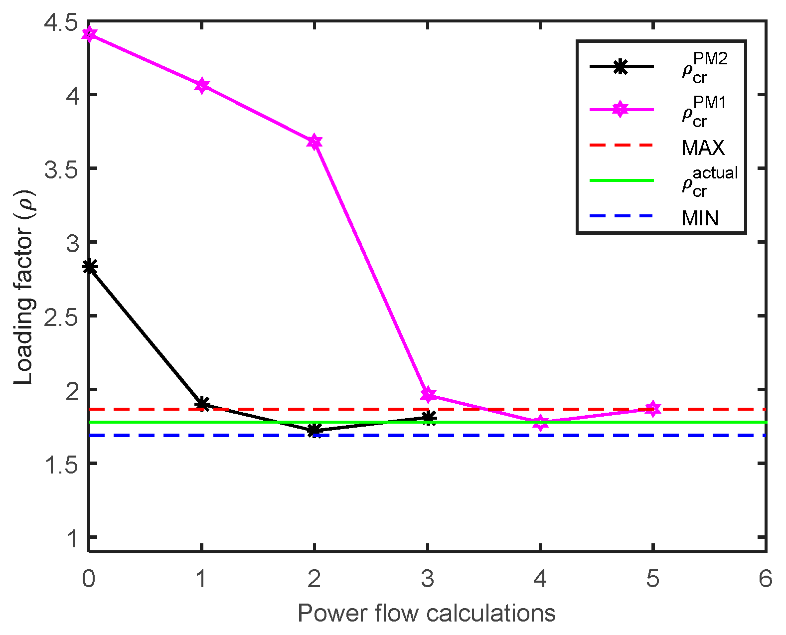
Figure 8 presents a comparison of the behavior of the loading factor as a function of the number of power flow runs for
PM1 and
PM2, using the IEEE 14-bus test system as an example, with
.
PM2 provides a faster solution, requiring only one iteration and three power flow runs.
4.2.2. Large Systems
Table 10 presents the performance of
PM2 for larger realistic systems [
28]. It is worth noting that
is now closer to the actual maximum loading, highlighting the advantage of incorporating generator sensitivities. Specifically, for the 2746 wp system,
lies within the feasible region, that is,
. This further underscores the robustness of the proposed method
PM2.
Figure 9 illustrates the evolution of the iterative process for the large systems listed in
Table 10, considering an acceptable error
.
4.3. Proposed Method and the Continuation Method
The literature presents several methods for determining the maximum loading of power systems. Most of these methods rely on tuning simulation parameters, which makes a fair comparison among them a challenging task. Considering this, the purpose of this section is to compare the performance of the proposed methods,
PM1 and
PM2, with the well-known continuation power flow (CPF). The CPF implementation from MATPOWER [
28] is regarded as a reliable simulation tool and has been widely adopted in power system research. Specific simulation conditions were defined to ensure the fairest possible comparison among the three methods, as outlined below.
Proposed methods PM1 and PM2—the acceptable error was defined as , matching the value used in the previous simulations.
CPF from MATPOWER—the default parameters were used (e.g., step size, tolerances, parameterization method). The iterative process was halted once the nose of the PV curve was reached, although MATPOWER can compute the complete PV curve. The reactive power limits of the generators were enforced. The active and reactive power limits of the slack bus were left open (). Additionally, the upper limit of active power for all PV buses (generators) was set to .
The CPF consists of two steps, namely a predictor and a corrector [
28]. The predictor step uses the tangent vector (MATPOWER’s default). The corrector step involves solving an augmented set of power flow equations, where an additional equation related to parameterization is included alongside the conventional ones. The computational burden of the CPF can generally be evaluated by the number of corrector steps (i.e., power flow-like runs) required to reach the nose point. CPF also features step size control, with a default step size of
. Additionally, it includes event functions (flags) that trigger a rollback when activated; that is, the current step is rolled back and retried with a modified step size. Rollbacks result in additional power flow-like runs.
The computational burden of the proposed methods can also be evaluated by the number of power flow runs with step size optimization (PFSSO). In turn, the computational effort of a PFSSO run is practically equivalent of that of a conventional power flow, as discussed in [
23].
Table 11 presents the results obtained for the IEEE standard test systems, as well as for a large system from MATPOWER [
28]. Rows 6, 10, and 13 from
Table 11 demonstrate that the proposed methods are able to converge to the actual maximum loading point, within the predefined acceptable error margin, after a small number of power flow runs.
It is important to note that this is not a complete comparison, since the simulations were based on specific parameter settings, as discussed earlier. For instance, if the acceptable error for
PM1 and
PM2 were smaller—say,
—the number of power flow runs would likely have been higher. Conversely, if the step size of CPF was larger—for example,
—the number of power flow-like runs would likely have been lower. The CPF results from
Table 11 were obtained by the following MATPOWER code:
| define_constants; |
| mpopt = mpoption(‘out.all’, 0,’verbose’, 2); |
| mpopt = mpoption(mpopt, ‘cpf.stop_at’, ‘NOSE’, ‘cpf.step’, 0.05); |
| mpopt = mpoption(mpopt, ‘cpf.plot.level’, 1); |
| mpopt = mpoption(mpopt, ‘cpf.enforce_q_lims’, 1); |
| mpopt = mpoption(mpopt, ‘cpf.plot.bus’, 9201); |
| mpcb = loadcase(case2869pegase); |
| mpct = mpcb; |
| mpct.gen(:, [PG QG]) = mpcb.gen(:, [PG QG]) * 2; |
| mpct.bus(:, [PD QD]) = mpcb.bus(:, [PD QD]) * 2; |
| results = runcpf(mpcb, mpct, mpopt); |
This particular code was applied to generate the PV curve of “case2869pegase” system from MATPOWER. Naturally, the code must be appropriately modified to obtain the PV curves for other systems.
5. Conclusions
This paper proposed two robust and efficient methods for determining the maximum loading factors and voltage stability margins of power systems. These methods were specifically designed for real-time operational applications. The core idea behind both approaches was to integrate two existing techniques from the literature, preserving their advantages while addressing their limitations.
A linear voltage stability index was used to establish the initial guess for an iterative method based on a non-divergent, robust, and second-order power flow with step size optimization. Subsequently, a loading factor derived from the sensitivity of loading with respect to the generators’ reactive powers was combined with that obtained from the linear voltage stability index. The resulting method proved to be even more efficient.
One of the key features of the proposed methods is their ability to handle different initial guesses. Simulation results have shown that the number of iterations is consistently low, regardless of whether the initial guess is feasible or infeasible, or close to or far from the actual MLP.
The maximum loading points of both the standard test systems and realistic power systems were computed after a small number of power flow runs. The efficiency of the proposed methods was demonstrated through a comparative analysis with the continuation power flow method, under specific assumptions regarding parameter settings.
