Abstract
Dynamic line rating (DLR) is an effective technique for real-time assessments on current-carrying capacities of overhead lines (OHLs), improving efficiencies and preventing overloads of transmission networks. Most research related to DLR forecasting mainly translates predictions of weather conditions into DLR forecasts or directly trains artificial intelligence models from DLR observations. Less attention has been given to the predictability of effective wind speeds (EWS) that describe overall convective cooling effects of varying weather conditions along OHLs, which could increase the reliability of DLR forecasts. To assess the effectiveness of EWS concepts in improving DLR predictions, this paper develops an EWS-based method for convective cooling predictions which are critical parameters dominating DLRs of overhead conductors. The EWS is first calculated from actual measurements of wind speeds and directions relative to OHL orientation based on the thermal model of overhead conductors. Then, an autoregressive model along with the Fourier series is employed to predict ultra-short-term EWS variations for up to three 10-min steps ahead, which are eventually converted into predictions of convective cooling effects along OHLs. The proposed EWS-based method is tested based on wind condition measurements in proximity to an OHL. Furthermore, to examine the impacts of angles between wind directions and line orientation on EWS estimation and thus EWS-based convective cooling predictions, the forecasting performance is assessed in the context of different line orientations. Results demonstrate that EWS-based ultra-short-term convective cooling predictions consistently outperform traditional forecasts from original wind conditions across all the tested line orientations. This highlights the significance of the EWS concept in reducing the complexity of DLR forecasting caused by the circular nature of wind directions, and in enhancing the accuracy of convective cooling predictions.
1. Introduction
The continuous growth of global energy demands together with the increasing integration of renewable energy sources heightens the requirement on secure, reliable and efficient operation of power systems. To accommodate constantly increasing loads on transmission networks, enhancing the utilisation efficiency and current-carrying capacities of existing overhead lines (OHLs) has emerged as a key challenge. Dynamic line rating (DLR), as an effective approach to exploiting the ampacity of transmission lines, has been widely researched in the context of high-voltage transmission networks [1]. Unlike traditional static ratings which are estimated from conservative ambient conditions, DLR techniques enable real-time assessments on OHL capacities under prevailing weather conditions, which can not only improve the OHL utilisation efficiency but also reduce the risk of OHL overloading, providing a cost-effective way to accommodate short-term growths of power flows [2].
In the main, DLR techniques utilise real-time meteorological data and sensor systems to calculate the maximum current-carrying capacities of OHLs. Compared with conventional static rating methods, DLR offers greater flexibility and accuracy in line ratings for the dispatch of power flows. Available DLR techniques can generally be categorised into two types: one based on weather data measured at or in close proximity to OHL conductors, and the other based on real-time monitoring of conductor temperature or other physical parameters such as tension or sag [3]. Weather-based DLR models typically perform DLR calculations of OHL conductors using real-time observations of air temperature, solar radiation wind speed and direction in combination with the thermal model of conductors [4]. Conductor temperature-based models, on the other hand, infer effective weather conditions experienced by the OHL from the monitored temperature changes, which are then fed into the thermal model of conductors for DLR estimation [5]. In practical application of DLR techniques, DLR data are generally provided in the form of predictions so that power system operators have time to make decisions on the dispatch of power flows in different time scales [6].
Most research related to DLR predictions applies statistical methods, machine learning algorithms and physics-based models to weather condition measurements or directly to DLR estimates. Conditionally heteroskedastic autoregressive (AR) models were developed in [7] for probabilistic forecasting of weather conditions, which were then translated into predictive distributions of DLRs via the thermal model of OHL conductors. In [8], the thermal inertia of OHL conductors was additionally considered to predict transient-state DLRs that result in the conductor temperature increasing to the maximum allowable level at the end of a 30 min horizon. A density forecasting method based on dynamic stochastic general equilibrium was proposed in [9], which offered narrower prediction intervals and higher reliability compared to machine learning and regression models in specific case studies. In [10], probabilistic day-ahead DLR prediction models were developed by training the quantile linear regression, mixture density neural networks, kernel density estimators or quantile regression forests (QRF), based on weather observations and numerical weather predictions (NWPs); the tree-based QRF forecasting method achieved good performance across all the metrics under tests including continuous ranked probability score, quantile score and sharpness of prediction intervals. QRF was also employed in [11] for day-ahead DLR forecasting. Given the large data sets generated by NWPs, principal component analysis was commonly used in [10,12] to reduce input redundancy in prediction models. In [13], a stacked and bagged ensemble model was proposed for weather-based DLR predictions, which outperformed single machine learning models in terms of bias and variance. In [14], a number of regression models including linear, nonlinear, regression trees and rule-based models were trained directly using historical DLR estimates to predict DLR across time horizons ranging from 30 min to 24 h, demonstrating that linear regression models might yield less accurate forecasts. In [15], partial autocorrelation analysis was conducted to determine the appropriate length of historical weather data for training a bidirectional long short-term memory model; resulting weather forecasts were then translated into DLR predictions via the thermal model of conductors. In [16], an algorithm combining K-means clustering with Monte Carlo simulation was proposed for short-term DLR forecasting, which outperformed quantile regression and recurrent neural network methods. In [17], a load flow modelling method combining machine learning with NWP was proposed for DLR forecasting over the next 27 h, which provided a satisfactory safety margin for day-ahead forecasts. Multilayer perceptron, group method data handling, support vector regression, back-propagation neural network, extreme learning machine (ELM) and hierarchical ELM (H-ELM) techniques were compared and evaluated in [18] where the H-ELM method had the lowest forecasting errors and the highest correlation coefficients. Additionally, the H-ELM method was reported to address the issue of single-point measurements, eliminating the need for additional sensors to be deployed along the line. In [19], a short-term weather forecasting method was developed based on an extended Kalman filter neural network, and then extended to obtain DLR forecasts using the heat balance equation.
Even though the aforementioned approaches have demonstrated their capability of DLR forecasting in particular timescales, less attention has been paid to the prediction of effective wind speed (EWS) perpendicular to OHLs. The concept of EWS is generally used to describe the average convective cooling effect experienced by an OHL along which wind speeds and directions would vary from span to span. It is particularly applied in the DLR techniques which infer DLRs from OHL status such as conductor temperature, sag or tension. While the role of EWS in DLR forecasting is less explored, the uncertainty progressing from real-time measurements to DLR estimation through the EWS has been investigated to correct DLR estimates. In [3], a Monte Carlo-based method was developed to deal with errors in conductor temperature measurements, mitigating the overestimation of EWS and resulting DLRs. In [20], different DLR monitoring methods relying on the concept of EWS are comprehensively reviewed, which convert measurements of conductor temperature, line tension or span sag into EWS and determine resulting DLRs during normal operation or emergency conditions.
The main contributions of the paper are to investigate the application of EWS in DLR predictions and examine the predictability of EWS and resulting convective cooling effects. To form a comparison between EWS-based convective cooling predictions against those that are inferred from forecasts of original wind speeds and directions, real-time observations of wind speeds and wind directions relative to line orientation are first translated into the time series of EWS that provides the same convective cooling effect on conductors. Then, ultra-short-term predictions for up to three 10 min steps ahead are generated for both EWS and original wind conditions using the Fourier series in conjunction with (vector) autoregressive models, which are responsible for diurnal trend extraction and residual forecasting, respectively. Finally, convective cooling effects are predicted from ultra-short-term forecasts of EWS or original wind conditions, through the thermal model of overhead conductors. The accuracies of convective cooling predictions estimated by the EWS-based and wind condition-based methods are assessed and compared in the cases of different line orientations to validate the potential accuracy improvement by the application of EWS in convective cooling forecasting. The EWS-based method proposed here provides a novel approach to improving DLR forecast accuracies and avoiding the modelling complexity related to the circular nature of wind directions.
The rest of the paper is structured as follows: Section 2 introduces the definition of EWS and its calculation from original wind speed and direction via the thermal model of overhead conductors; Section 3 describes the ultra-short-term forecasting of EWS or wind speeds and directions by the joint use of the Fourier series and (vector) AR models; Section 4 discusses and compares predictions of EWS and original wind conditions, as well as their resulting convective cooling effects on OHL conductors under different line orientations; Section 5 discusses the advantages of the EWS-based method for convective cooling predictions; and conclusions and recommendations for future work are presented in Section 6.
2. Effective Wind Speed Modelling
2.1. Concept of Effective Wind Speed
The concept of EWS is generally applied in the DLR techniques that rely on the monitoring of OHL status such as conductor temperature, sag or tension. The EWS is assumed to be perpendicular to the OHL and result in the same convective cooling effect as actual wind conditions. It can not only more accurately describe the convective cooling effect on overhead conductors, but is also of particular interest to the OHL sections that cross multiple terrains and experience various wind conditions, in which case the EWS could represent the average convective cooling effect of varying wind conditions on the entire OHL. By employing the thermal model of overhead conductors such as IEEE 738 Standard [4], the EWS can be derived from observations of line current, air temperature and solar radiation in combination with conductor temperature directly measured or indirectly inferred from sag or tension measurements, as shown in Figure 1. In general, the EWS which affects convective heat losses is calculated to reflect the monitored conductor temperature under steady state or the continuous variation of monitored conductor temperature under transient state, as formulated by (1) or (2), respectively.
where , and represent rates of convective heat loss, radiative heat loss and solar heat gain of the conductor per unit length, respectively; is the current passing through the conductor; and denote the AC resistance and heat capacity of the conductor per unit length; is the conductor temperature under steady state; and and are initial and final conductor temperature over a time step length of under transient state. Please refer to IEEE 738 Standard [4] for more details of the steady-state or transient-state thermal model of overhead conductors.
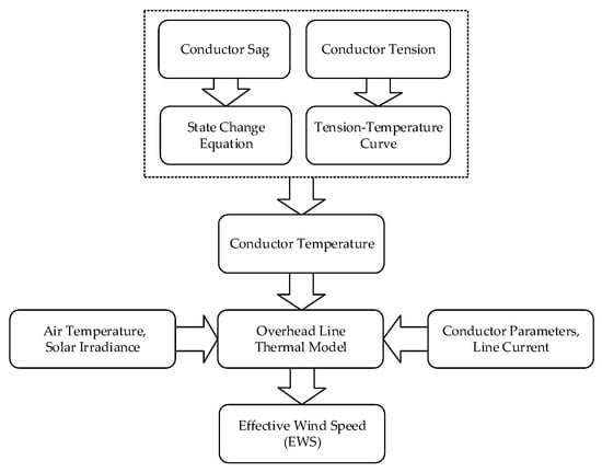
Figure 1.
Processes of the EWS estimation from conductor temperature measurements or inferences from sag or tension.
2.2. Specific Estimation of Effective Wind Speed
As was noted in Section 2.1, the EWS influences the convective heat loss rate only in the thermal model of overhead conductors. To assess the predictability of EWS and compare the EWS-based forecasting method with those that are inferred from actual wind conditions, the time series of EWS is estimated from measurements of wind speeds and directions in this work by assuming that the EWS provides the same cooling effect as wind speeds and directions. Convective heat loss is generally divided into two types, i.e., natural convection and forced convection. According to IEEE Standard 738 [4], natural convection occurs under stagnant air conditions and can be formulated by Equation (3). Forced convection is represented by either Equation (4) or (5). Equation (4) is used to calculate convective heat loss rate under low wind speeds, i.e., in the case of low Reynolds numbers . Equation (5) applies to the calculation of convective heat loss rate under high wind speeds, i.e., in the case of high .
where is the air density, denotes the conductor’s outer diameter, and and are the conductor surface temperature and ambient temperature, respectively. The Reynolds number representing the ratio of inertial forces to viscous or frictional forces in wind speed is formulated by Equation (6), where is the air viscosity.
The wind direction factor is expressed by Equation (7) to characterise the impact of the difference between wind direction and line orientation on convective heat loss. Thermal conductivity varies with physical properties of the medium. In heat transfer, the thermal conductivity of air depending on the boundary layer temperature can be calculated using Equation (8) which is empirically derived from experimental data.
where represents the average temperature of the boundary layer, which can be calculated by .
Even though convective heat loss rates are defined by Equations (3)–(5) for different wind speed conditions, there lack specific boundaries differentiating the wind speed condition for the exact selection of , or . In addition, the coupling of natural and forced convections becomes significantly pronounced under low wind speed conditions, meaning more complex heat exchange processes. According to McAdams [21], the higher of or shall be selected for wind speeds above zero, while the higher of or could be selected for null or low wind conditions as a conservative estimate. To that end, the convective heat loss rate would be calculated by combining Equations (3)–(5) and taking the maximum of their resulting rates. This is formulated by Equation (9).
Given the determined from wind speed and direction measurements, the corresponding EWS perpendicular to overhead conductors (i.e., resulting in ) is calculated to replicate the same . It is noted that the EWS is set to 0 m/s when the is dominated by the natural convection which does not rely on wind conditions. The calculation of EWS is formulated by Equation (10) which are derived from Equations (3)–(5).
3. Ultra-Short-Term Wind Forecasting
3.1. Ultra-Short-Time EWS Forecasting
3.1.1. Temporal Trend Modelling
Statistical models such as AR models typically require the input data to satisfy weak or second-order stationarity. This means that the average and variance of the input data should remain constant over time, while its autocovariance depends only on the time lag. When the input data which often contain some trend components are non-stationary, the true relationships between variables could be obstructed, misleading the analysis of time series autocorrelation. Therefore, it is essential to detrend the data by removing its inherent trend(s) prior to the application of statistical models.
In this study, the Fourier series is used for temporal de-trending [22]. By selecting the Fourier series of an appropriate order, the temporal trend component(s) can be extracted and removed from the input data of EWS. This is formulated by Equation (11):
where is the fundamental (diurnal) angular frequency equalling ; and and represent the offset in input data and the amplitude of the th harmonic (). In this way, periodic variations in data can be effectively preserved and removed, thereby improving the performance of subsequently applied statistical models.
3.1.2. Autoregressive Model
The AR-based time series forecasting model is developed here to calculate point forecasts of the residuals of EWS by capturing the auto-correlation from historical time series. A -order AR process with a time lag of is a stochastic model estimating the residual forecast for step(s) ahead as a linear combination of historical values and a Gaussian noise term denoted by [22]. This can be formulated by Equation (12).
where denotes the residual of the variable exclusive of temporal detrends; is a constant; and are the AR parameters which can be determined using ordinary least squares estimation [23]. Given the time series of residuals in preparation for AR parameter estimation, a set of AR processes with a time lag of can be defined in the form of Equation (12), as formulated by Equation (13).
which can be written in matrix form, as shown in Equation (14).
where
Then, the constant and AR parameters can be estimated using Equation (15).
Finally, the residual forecast estimated from the optimised AR model is combined with its corresponding temporal trend to determine the point forecast of the variable. Figure 2 shows a flowchart describing the processes of ultra-short-term forecasting with the joint use of the AR model and temporal de-trending.
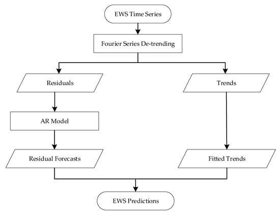
Figure 2.
Processes of the variable prediction by AR models with temporal de-trending.
3.2. Ultra-Short-Time Forecasting of Wind Speeds and Directions
3.2.1. Vector Autoregressive Model
To validate the effectiveness of the EWS-based method for ultra-short-term forecasting of convective heat loss rates, the methods relying on predictions of wind speeds and directions are additionally developed in this work by also utilising AR models. However, since a conventional AR model is applied to a single variable only, it cannot adequately capture the coupling relationship between wind speeds and directions. In addition, the circular nature of wind directions makes it inappropriate to directly apply an AR model which is suitable for linear time series. To address these issues, wind direction can be decomposed along horizontal and longitudinal axes within the Cartesian coordinate. The resulting horizontal and longitudinal components are then fed into a vector AR (VAR) model which simultaneously model multiple variables by accounting for their mutual dependencies.
As an extension of the univariate AR model, a VAR model of order p provides a forecasting framework by utilising a weighted sum of historical time series not only from the variable itself but also from () other related variables [24]. The VAR process can be formulated by
where is a (K × 1) vector comprising residuals of variables (j = 1, …, K); is a (K × 1) vector comprising constants of residuals of variables; represents a (K × K) matrix consisting of VAR parameters at time lag (); and is a (K × 1) vector of noise terms [24].
In order to determine VAR model parameters through the multivariate least square estimation, the residual time series of variables are used to formulate Equation (17) in the matrix form.
where
Then, VAR parameters together with constants are determined by minimising the sum of squares of noise terms or .
3.2.2. Decomposition of Wind Directions
Two different methods of wind direction decomposition are employed here prior to the application of VAR models, as shown in Figure 3a,b. The two decomposition methods, in turn, lead to two different VAR-based approaches for forecasting of wind speeds and directions.
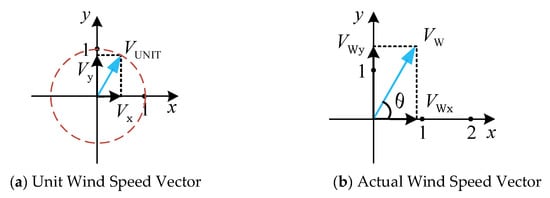
Figure 3.
Wind direction decomposition within the Cartesian coordinate based on (a) unit wind speed or (b) actual wind speed.
In the first VAR-based approach (referred to as VAR1), wind speed is forecast in the same way as the EWS by jointly using an AR model with temporal de-trending, while wind direction is decomposed by constructing a unit wind speed vector and projecting it onto the Cartesian coordinate to obtain horizontal and longitudinal components (see Figure 3a). Given the strong correlation between the two components, a VAR model is then employed to estimate their joint predictions, from which the ultra-short-term wind direction prediction is reconstructed.
In contrast to the VAR1 approach where wind speed and direction are predicted separately, the second VAR-based approach (referred to as VAR2) constructs the wind speed vector based on actual wind speed (see Figure 3b) instead of unit wind speed and decomposes it along horizontal and longitudinal directions within the Cartesian coordinate. The two components are then jointly modelled and predicted by using a VAR model. The resulting predictions of the two components are then translated into ultra-short-term predictions of wind speeds and directions.
4. Results
The ultra-short-term predictability of EWS is examined here based on 10 min average wind speeds and directions observed at a particular weather station in close proximity to OHLs over 2017–2018. This section first presents real-time EWS estimation from wind condition observations and illustrates their distributions and temporal trends. Then, EWS forecasts for up to three steps ahead estimated by the EWS-based, VAR1 or VAR2 method are assessed in terms of root mean absolute error (RMSE), and further compared against persistence forecasting [25] to demonstrate the predictability of EWS and the performance of different methods under tests. Considering the variation of line orientation will alter the attach angle between wind direction and line and thus affect the EWS estimation, the evaluation on characteristics and predictability of EWS are conducted under different line orientations, respectively, to examine the influences of line orientation.
4.1. EWS Estimation from Wind Condition Measurements
Figure 4 shows measurements of wind speeds and directions during a particular day. The overall distributions of wind speeds and directions measured over the two years are shown in Figure 5. For the weather station selected in this work, the wind directions along NNW, SE and SSW are more frequent throughout the two years. Furthermore, the wind directions along NNW and SSW are relatively more concentrated and their accompanying wind speeds are higher in part due to the local terrain. In the main, the actual wind speed measurements are distributed within 0–15 m/s. In order to examine the effects of line orientation or wind attach angle on EWS characteristics and predictability, four different line orientations of 0° (along Eastward), 30° (along ENE), 60° (along NNE) and 90° (along Southward) are adopted in this work. By using the specific EWS estimation method described in Section 2.2, the EWS that results in the same cooling effect on overhead conductors of 0° orientation as actual wind conditions is calculated. Due to the fact that the EWS assumes an attack angle of 90° which maximises the convective heat loss rate brought by a given wind speed, the EWS is shown to be smaller than or equal to the actual wind speed for all the time, as shown in Figure 6.
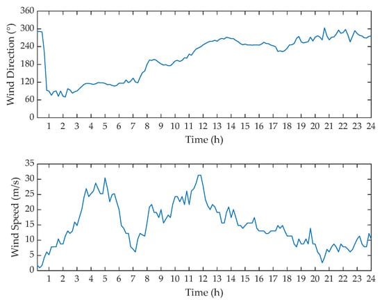
Figure 4.
Wind speed and wind direction profiles measured over a particular day.
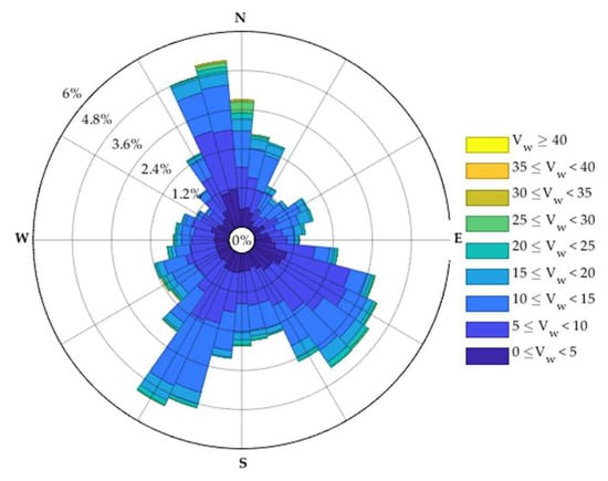
Figure 5.
Distributions of wind speed and wind direction measurements over two years.
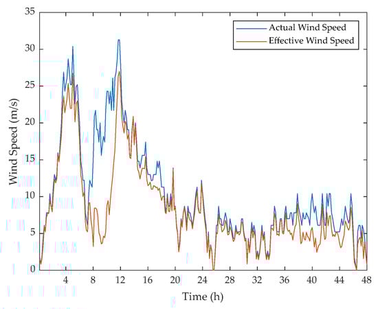
Figure 6.
Comparison of actual and effective wind speed in the case of the 0° line orientation.
Figure 7 shows the distributions of the EWS estimates over the two years in the cases of different line orientations. As was noted above, since the EWS is always smaller than or equal to actual wind speed, the overall distribution of the EWS is found to skew more to the left compared to actual wind speed. In addition, when the line orientation is assumed to be 60° or 90°, there exists a wind direction cluster where wind directions are almost parallel to the line orientation (see Figure 5), which mitigates convective cooling effects and thus results in lower EWS. To that end, the amplitudes of EWS in the case of 0° or 30° line orientation are estimated to be greater on average than in the case of 60° or 90° line orientation. To quantitatively validate the difference in EWS between the four line orientations on average, the EWS distribution for each line orientation is modelled by the Gamma distribution which was found to provide better fitting than the Weibull distribution. The estimated shape () and scale () parameters as well as corresponding mean values () are listed in Table 1. Notably, the shape parameters of EWS distributions are estimated to be less than or equal to 2.03, which are smaller than the shape parameter of 2.65 estimated for the Gamma distribution of original wind speeds. This indicates the left-skewed nature of the EWS distribution as discussed above. In addition, the mean values of EWS decrease progressively from the 0° or 30° orientation to the 60° or 90° orientation, quantitatively confirming that EWS amplitudes are greater on average when more wind directions are almost perpendicular to the line orientation, and vice versa.
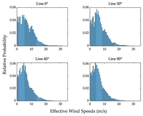
Figure 7.
Distributions of effective wind speed estimated under different line orientations.

Table 1.
Shape parameters (dimensionless) and scale parameters (m/s) as well as mean values (m/s) of the Gamma distributions fitted to EWS data given different line orientations.
4.2. Determination of AR Order for EWS Forecasting
The order of the AR model should be appropriately selected to deal with the trade-off between forecast accuracy and computational costs. The time series of EWS estimates over the first eight months is used as the training set to determine the AR order that cannot further improve forecast accuracy. As was noted in Section 3.1.1, in order to ensure the second-order stationary of time series applied to AR models, the diurnal trend of the EWS in the case of each line orientation is modelled using the Fourier series, as shown in Figure 8, and then removed from the EWS time series to obtain the residuals. The diurnal trends of EWS are generally similar between different line orientations, though the periodic variations of EWS are more pronounced in the cases of 0° and 30° line orientations where the EWS amplitudes are higher on average than those in the cases of 60° and 90° line orientations. In addition, the peaks of diurnal EWS trends are shown to occur between 14:00 and 17:00 on average due to the fact that the original wind speeds recorded in the coastal city tend to be higher during the afternoon hours.
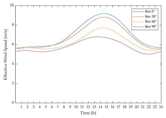
Figure 8.
Diurnal trends of EWS time series estimated under different line orientations.
The RMSE of persistence forecasts is adopted here as the benchmark to examine the performance of different AR models in ultra-short-term predictions for up to three steps ahead. Figure 9 shows the improvement of AR models with different orders in RMSE over persistence in the case of 0° line orientation. The improvement over persistence is shown to increase not only with the order of the AR model, but also with the increase in forecast horizon. It is found that the use of an AR order above 7 can hardly further improve the performance of EWS predictions for up to three steps ahead under all the line orientations. To that end, the AR model orders are determined to be 7 for all the forecast horizons and line orientations in this work.
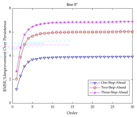
Figure 9.
Improvement of AR models with different orders in RMSE over persistence for up to three steps ahead in the case of 0° line orientation.
4.3. Ultra-Short-Term Forecasting of Effective Wind Speed
Figure 10 shows the EWS forecasts for up to three steps ahead against the actual EWS estimates during a particular day in the case of 0° line orientation. In the main, ultra-short-term EWS forecasts follow the variations of actual EWS estimates and present a good consistency. To quantitively assess the performance of AR models against persistence, RMSE values of EWS predictions for up to three steps ahead estimated by AR models and the persistence forecast method under different line orientations are tabulated in Table 2 and Table 3, respectively. Furthermore, the percentage improvement of AR models over persistence in RMSE for up to three steps ahead is illustrated in Figure 11 where the improvement over persistence increases with the forecast horizon. The improvement of AR models over persistence is similar between different line orientations, though slightly higher improvement is achieved in the case of 0° line orientation for one-step-ahead EWS forecasts and in the case of 30° line orientation for two- and three-step-ahead EWS forecasts.
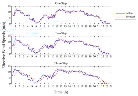
Figure 10.
Ultra-short-term EWS predictions for up to three steps against actual EWS estimates in the case of 0° line orientation.
Table 2.
RMSE values (in m/s) of EWS predictions for up to three steps ahead by AR models’ forecast method under different line orientations.
Table 3.
RMSE values (in m/s) of EWS predictions for up to three steps ahead by persistence forecast method under different line orientations.
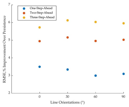
Figure 11.
Improvement of AR models over persistence in RMSE of EWS predictions for up to three steps ahead under different line orientations.
4.4. Convective Heat Loss Forecasting by Different Methods
By using Equations (3)–(9), the EWS predictions together with 90° wind attack angles are translated into the corresponding forecasts of convective heat loss rates which are generally the dominant factors that influence DLR predictions. In addition to the EWS-based approach to convective heat loss forecasting, the VAR1- and VAR2-based methods which decompose wind directions in different ways (as was described in Section 3.2.2) are applied to predict convective heat loss rates for up to three steps ahead as a comparison. Figure 12 shows the ultra-short-term predictions of convective heat loss rates estimated by the EWS-, VAR1- and VAR2-based methods against actual estimates of convective heat loss rates in the case of 0° line orientation during a particular day. In the main, the three methods show a good consistency in ultra-short-term predictions of convective heat loss rates and all replicate the variations of actual convective heat loss rates.
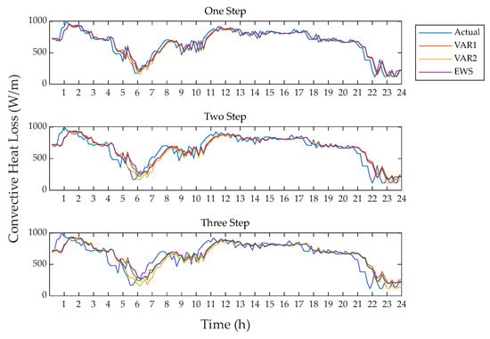
Figure 12.
Convective heat loss rates predicted by EWS-, VAR1- and VAR2-based methods for up to three steps ahead against the actual estimates in the case of 0° line orientation.
Table 4 lists RMSE values of convective heat loss rates predicted by the three different methods for up to three steps ahead in the cases of the four line orientations. For each line orientation, the EWS-based method is shown to perform similarly or even better than the two VAR-based methods that rely on original wind speeds and wind directions. In addition, the VAR1-based method which decomposes unit wind speed vectors within the Cartesian coordinate provides more accurate forecasts of convective heat loss rates than the VAR2-based method which splits the actual wind speed vectors. This suggests that individually forecasting wind speeds and directions is preferred for DLR studies in this work. To illustratively compare the prediction accuracy between the three methods, the percentage improvement of EWS- and VAR1-based methods in RMSE values of convective heat loss rate forecasts over the VAR2-based method is estimated for each line orientation, as shown Figure 13.
Table 4.
RMSE values (in W/m) for short-term forecasting of convective heat loss rate under different line orientations.
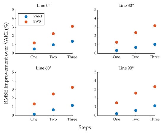
Figure 13.
The percentage improvement of EWS- and VAR1-based methods over the VAR2-based method in RMSE for predictions of convective heat loss rates under different line directions.
Compared with the VAR2-based method, both VAR1- and EWS-based methods exhibit significant improvements in terms of RMSE for all the line orientations under tests. It is noted that the VAR1-based method shows more pronounced improvement when the line orientation equals 0° or 30° where there are less significant clusters of wind directions that are parallel to the line orientation (see Figure 5). This is because wind directions being less parallel to line orientation increase the dependency of convective heat loss rates on wind speeds, and vice versa. To that end, the accurate wind speed forecasts of the VAR1-based method are more reflected in the convective heat loss rate forecasts under 0° or 30° line orientation than under 60° or 90° line orientation. In contrast, the EWS-based method achieves superior RMSE reductions consistently for all the line orientations, significantly outperforming the two VAR-based methods. This highlights the potential robustness and applicability of the EWS-based forecasting method for convective heat loss rates in DLR studies.
5. Discussion
The proposed EWS-based method, which shows its enhancement in convective heat loss rate forecasting over the conventionally used VAR1- or VAR2-based method, can then be combined with forecasts of radiative heat loss and solar heat gain rates for the eventual DLR forecasts. Since radiative heat loss and solar heat gain rates are independent of wind conditions, the improvement of convective heat loss rate forecasts achieved by the EWS-based method proposed here will lead to more accurate DLR predictions. In addition to the accuracy improvement, the use of the EWS concept can avoid dealing with the circular nature of wind direction, which would largely simplify the development of DLR forecasting algorithms, especially in the cases of evaluating probabilistic forecasts or predictive distributions of DLRs. When the VAR1- or VAR2-based method is applied to probabilistic DLR forecasting, the wind direction samples randomly produced in the Monte Carlo simulation must be paired with other weather variables so as to reflect their correlations that are implied in their historic data. However, traditional pairing methods of linear variables cannot deal with the circular nature of wind direction, while the methods suitable for circular data, such as circular copula, are complex to be implemented. Therefore, the use of the EWS can not only improve the DLR prediction accuracy, but also facilitate the pairing process which involves linear variables only.
It is noted that the concept of EWS is normally applied for the DLR techniques that rely on direct measurement of indirect inference of conductor temperature. In such cases, the EWS value is estimated to replicate the monitored conductor temperature or its variation based on the thermal model of overhead conductors given the simultaneous measurements of line current, air temperature and solar radiation. Then, AR models proposed in this work can be used for the ultra-short-term EWS predictions. Even though the EWS concept is mainly considered by the conductor temperature-, sag- or tension-based DLR technique, the benefits of inferring EWS from original wind speed and direction and then directly predicting EWS for convective heat losses are highlighted in this work. This provides a new, accurate and simple approach to DLR forecasting for the weather-based DLR techniques.
6. Conclusions
Effective wind speed (EWS) is a critical concept in dynamic line rating (DLR) studies, though less attention is given to EWS in the field of DLR forecasting. This paper has proposed a forecasting method for convective heat loss rates by using the concept of the EWS, with the objective of improving the forecast accuracy and avoiding the model complexity induced by the circular nature of wind direction. By deriving the linear EWS from original wind speeds and directions with respect to specific line orientations, the method circumvents the inherent circularity of wind direction, thereby enabling the direct application of autoregressive (AR) models for ultra-short-term EWS forecasting which is then converted into convective heat loss rate predictions. In addition, the traditional forecasting methods which decompose unit or actual wind speed vectors within the Cartesian coordinate have been developed by using vector AR (VAR) models as a comparison.
The EWS- and VAR-based forecasting methods have been tested based on actual observations of wind speeds and directions at a particular weather station in close proximity to an overhead line (OHL). Comparative analysis indicated that the proposed EWS-based method consistently outperformed conventional VAR-based methods under various line orientations, demonstrating superior accuracy and stability in convective heat loss predictions. In addition to the enhancement in forecasting accuracy, the introduction of the EWS significantly reduces modelling complexity related to the circular nature of wind direction. Traditional approaches must address the circular nature of wind direction and its correlations with other meteorological variables, often relying on complex mathematical tools that are computationally demanding and difficult to implement. The EWS-based method proposed here is particularly well suited for the DLR applications that require high computational efficiency and real-time responsiveness. It provides a novel, accurate and practical approach to weather-based DLR forecasting, offering new theoretical insights and methodological support for the development of weather-based DLR techniques.
Building on the present work, the proposed EWS-based forecasting method will be integrated with predictions of radiative heat loss and solar heat gain to form a complete weather-based DLR forecasting framework. Furthermore, the EWS-based method will be extended to model uncertainties of convective heat loss rate forecasts, contributing to the probabilistic DLR forecasting. In addition, the predictability of the EWS and resulting convective heat loss rates will be tested for the DLR techniques that rely on measurements of conductor temperature, sag or tension, and validated in practical applications.
Author Contributions
Conceptualization, F.F. and K.S.; methodology, Y.W. (Yuxuan Wang) and F.F.; software, Y.W. (Yuxuan Wang) and F.F.; validation, Y.W. (Yuxuan Wang) and F.F.; formal analysis, Y.W. (Yuxuan Wang) and F.F.; investigation, Y.W. (Yuxuan Wang), F.F., Y.W. (Yu Wang), K.W., J.J., C.S., R.X. and K.S.; resources, F.F., Y.W. (Yu Wang), K.W. and K.S.; data curation, Y.W. (Yuxuan Wang) and F.F.; writing—original draft preparation, Y.W. (Yuxuan Wang) and F.F.; writing—review and editing, Y.W. (Yu Wang), K.W., J.J., C.S., R.X. and K.S.; visualization, Y.W. (Yuxuan Wang); supervision, F.F. and K.S.; project administration, F.F., Y.W. (Yu Wang), K.W. and K.S.; funding acquisition, F.F. and K.S. All authors have read and agreed to the published version of the manuscript.
Funding
This research was funded by the State Key Laboratory of Technology and Equipment for Defense against Power System Operational Risks, grant number SGNRGF00SXQT2501974.
Data Availability Statement
The data presented in this study are available on request from the corresponding author. (The data are not publicly available due to privacy restrictions).
Conflicts of Interest
Author Fulin Fan was a visiting professor at the Nari Technology Co., Ltd. Authors Yu Wang and Ke Wang were employed by the Nari Technology Co., Ltd. Authors Yu Wang and Ke Wang were employed by the State Grid Electric Power Research Institute. The remaining authors declare that the research was conducted in the absence of any commercial or financial relationships that could be construed as a potential conflict of interest.
Abbreviations
The following abbreviations are used in this manuscript:
| DLR | Dynamic Line Rating |
| OHLs | Overhead Lines |
| EWS | Effective Wind Speed |
| AR | Autoregressive |
| QRF | Quantile Regression Forests |
| NWPs | Numerical Weather Predictions |
| ELM | Extreme Learning Machine |
| H-ELM | Hierarchical Extreme Learning Machine |
References
- Xiao, R.; Xiang, Y.; Wang, L.; Xie, K. Power System Reliability Evaluation Incorporating Dynamic Thermal Rating and Network Topology Optimization. IEEE Trans. Power Syst. 2018, 33, 6000–6012. [Google Scholar] [CrossRef]
- Su, Y.; Tan, M.; Teh, J. Short-Term Transmission Capacity Prediction of Hybrid Renewable Energy Systems Considering Dynamic Line Rating Based on Data-Driven Model. IEEE Trans. Ind. Applicat. 2025, 61, 2410–2420. [Google Scholar] [CrossRef]
- Fan, F.; Stephen, B.; Bell, K.; Infield, D.; McArthur, S. Impacts of Measurement Errors on Real-Time Thermal Rating Estimation for Overhead Lines. IEEE Trans. Power Deliv. 2023, 38, 1086–1096. [Google Scholar] [CrossRef]
- 738TM-2012; IEEE Standard for Calculating the Current-Temperature Relationship of Bare Overhead Conductors (Revision of IEEE Std 738-2006/Incorporates IEEE Std 738-2012/Cor 1-2013). IEEE: Piscataway, NJ, USA, 2013.
- Foss, S.D.; Maraio, R.A. Dynamic Line Rating in the Operating Environment. IEEE Trans. Power Deliv. 1990, 5, 1095–1105. [Google Scholar] [CrossRef]
- Douglass, D.A.; Grant, I.; Jardini, J.A.; Kluge, R.; Traynor, P.; Davis, C.; Gentle, J.; Nguyen, H.-M.; Chisholm, W.; Xu, C.; et al. A Review of Dynamic Thermal Line Rating Methods with Forecasting. IEEE Trans. Power Deliv. 2019, 34, 2100–2109. [Google Scholar] [CrossRef]
- Fan, F.; Bell, K.; Infield, D. Probabilistic Real-Time Thermal Rating Forecasting for Overhead Lines by Conditionally Heteroscedastic Auto-Regressive Models. IEEE Trans. Power Deliv. 2017, 32, 1881–1890. [Google Scholar] [CrossRef]
- Fan, F.; Bell, K.; Infield, D. Transient-State Real-Time Thermal Rating Forecasting for Overhead Lines by an Enhanced Analytical Method. Electr. Power Syst. Res. 2019, 167, 213–221. [Google Scholar] [CrossRef]
- Madadi, S.; Mohammadi-Ivatloo, B.; Tohidi, S. Probabilistic Real-Time Dynamic Line Rating Forecasting Based on Dynamic Stochastic General Equilibrium with Stochastic Volatility. IEEE Trans. Power Deliv. 2021, 36, 1631–1639. [Google Scholar] [CrossRef]
- Dupin, R.; Kariniotakis, G.; Michiorri, A. Overhead Lines Dynamic Line Rating Based on Probabilistic Day-Ahead Forecasting and Risk Assessment. Int. J. Electr. Power Energy Syst. 2019, 110, 565–578. [Google Scholar] [CrossRef]
- Cheng, Y.; Liu, P.; Zhang, Z.; Dai, Y. Real-Time Dynamic Line Rating of Transmission Lines Using Live Simulation Model and Tabu Search. IEEE Trans. Power Deliv. 2021, 36, 1785–1794. [Google Scholar] [CrossRef]
- Bosisio, A.; Berizzi, A.; Le, D.-D.; Bassi, F.; Giannuzzi, G. Improving DTR Assessment by Means of PCA Applied to Wind Data. Electr. Power Syst. Res. 2019, 172, 193–200. [Google Scholar] [CrossRef]
- Ahmadi, A.; Taheri, S.; Ghorbani, R.; Vahidinasab, V.; Mohammadi-ivatloo, B. Decomposition-Based Stacked Bagging Boosting Ensemble for Dynamic Line Rating Forecasting. IEEE Trans. Power Deliv. 2023, 38, 2987–2997. [Google Scholar] [CrossRef]
- Fernandez Martinez, R.; Alberdi, R.; Fernandez, E.; Albizu, I.; Bedialauneta, M.T. Improvement of Transmission Line Ampacity Utilization via Machine Learning-Based Dynamic Line Rating Prediction. Electr. Power Syst. Res. 2024, 236, 110931. [Google Scholar] [CrossRef]
- Song, T.; Teh, J. Dynamic Thermal Line Rating Model of Conductor Based on Prediction of Meteorological Parameters. Electr. Power Syst. Res. 2023, 224, 109726. [Google Scholar] [CrossRef]
- Lawal, O.A.; Teh, J. Dynamic Line Rating Forecasting Algorithm for a Secure Power System Network. Expert Syst. Appl. 2023, 219, 119635. [Google Scholar] [CrossRef]
- Aznarte, J.L.; Siebert, N. Dynamic Line Rating Using Numerical Weather Predictions and Machine Learning: A Case Study. IEEE Trans. Power Deliv. 2017, 32, 335–343. [Google Scholar] [CrossRef]
- Mansour Saatloo, A.; Moradzadeh, A.; Moayyed, H.; Mohammadpourfard, M.; Mohammadi-Ivatloo, B. Hierarchical Extreme Learning Machine Enabled Dynamic Line Rating Forecasting. IEEE Syst. J. 2022, 16, 4664–4674. [Google Scholar] [CrossRef]
- Sun, X.; Luh, P.B.; Cheung, K.W.; Guan, W. Probabilistic Forecasting of Dynamic Line Rating for Over-Head Transmission Lines. In Proceedings of the 2015 IEEE Power & Energy Society General Meeting, Denver, CO, USA, 26–30 July 2015; pp. 1–5. [Google Scholar]
- Douglass, D.; Chisholm, W.; Davidson, G.; Grant, I.; Lindsey, K.; Lancaster, M.; Lawry, D.; McCarthy, T.; Nascimento, C.; Pasha, M.; et al. Real-Time Overhead Transmission-Line Monitoring for Dynamic Rating. IEEE Trans. Power Deliv. 2016, 31, 921–927. [Google Scholar] [CrossRef]
- McAdams, W.H. Heat Transmission, 3rd ed; McGraw-Hill: New York, NY, USA, 1954. [Google Scholar]
- Shi, Y.; Zhang, L.; Sheng, Y. Ridge Estimation of Uncertain Vector Autoregressive Model with Imprecise Data. J. Ambient Intell. Human Comput. 2024, 15, 2143–2152. [Google Scholar] [CrossRef]
- Lee, M.; Han, C. Ordinary Least Squares and Instrumental-Variables Estimators for Any Outcome and Heterogeneity. Stata J. Promot. Commun. Stat. Stata 2024, 24, 72–92. [Google Scholar] [CrossRef]
- Mignon, V. Principles of Econometrics: Theory and Applications; Classroom Companion: Economics; Springer: Cham, Switzerland, 2024; ISBN 978-3-031-52534-6. [Google Scholar]
- Fan, F.; Bell, K.; Infield, D. Probabilistic Weather Forecasting for Dynamic Line Rating Studies. In Proceedings of the 2016 Power Systems Computation Conference, Genoa, Italy, 20–24 June 2016; pp. 1–7. [Google Scholar]
Disclaimer/Publisher’s Note: The statements, opinions and data contained in all publications are solely those of the individual author(s) and contributor(s) and not of MDPI and/or the editor(s). MDPI and/or the editor(s) disclaim responsibility for any injury to people or property resulting from any ideas, methods, instructions or products referred to in the content. |
© 2025 by the authors. Licensee MDPI, Basel, Switzerland. This article is an open access article distributed under the terms and conditions of the Creative Commons Attribution (CC BY) license (https://creativecommons.org/licenses/by/4.0/).