Article

Evaluation of XGBoost and ANN as Surrogates for Power Flow Predictions with Dynamic Energy Storage Scenarios

by
Perez Yeptho
*,
Antonio E. Saldaña-González
,
Mònica Aragüés-Peñalba
and
Sara Barja-Martínez
Centre d’Innovació Tecnològica en Convertidors Estàtics i Accionaments, Department d’Enginyeria Elèctrica, Universitat Politècnica de Catalunya, Av. Diagonal 647, 08028 Barcelona, Spain
*
Author to whom correspondence should be addressed.
Energies 2025, 18(16), 4416; https://doi.org/10.3390/en18164416
Submission received: 11 July 2025 / Revised: 5 August 2025 / Accepted: 11 August 2025 / Published: 19 August 2025

Abstract

Power flow analysis is essential for managing power systems, helping grid operators ensure reliability and efficiency. This paper explores the use of machine learning (ML) techniques as surrogates for computationally intensive power flow calculations to evaluate the effects of distributed energy resources, such as battery energy storage systems (BESSs), on grid performance. In this paper, a case study is presented where XGBoost (eXtreme Gradient Boosting) and Artificial Neural Networks (ANNs) are trained to simulate power flows in a medium-voltage grid in Norway. The impact of BESS units on line loading, transformer loading, and bus voltages is estimated across thousands of configurations, with results compared in terms of simulation time, error metrics, and robustness. In this paper it is proven that while ML models require considerable data and training time, they offer speed-up factors of up to 45×, depending on the predicted parameter. The proposed methodology can also be used to assess the impact of other grid-connected assets, such as small-scale solar plants and electric vehicle chargers, whose presence in distribution networks continues to grow.

1. Introduction

1.1. Background

According to the net zero scenario for the global energy transition, by 2030 the total installed grid-scale battery capacity is expected to reach 967 GW, up from 28 GW in 2022 [1]. Grid-scale batteries or BESSs, which are defined as a type of distributed energy resource (DER) by the IEA [2], will play a critical role in the energy grids of the future. DERs also include renewable energy plants, electric vehicles with vehicle-to-grid technology, and fuel cells, which are typically smaller in scale and distributed across multiple locations within the grid. In addition to providing energy storage itself, BESSs can provide additional services such as demand response, energy arbitrage, and grid stabilization. Using BESSs to stabilize the grid is well documented [3] such as when BESSs can be used to reduce transformer overloading [4,5] during peak load periods when demand is significantly higher than the rated capacity of the transformer. Studies have examined the technical feasibility and benefits of using BESSs to increase transmission capacity in regions with significant renewable energy generation [6]. Clearly BESSs will be increasingly important in the future and it becomes important to simulate grids during the planning phase of installation of any BESS. Currently, grid operators use power flow tools such as pandapower [7], DIgSILENT PowerFactory [8], and PowerWorld [9], along with other commercial and open-source software (verison 3.1.2). These tools are utilized to predict the impact that modifications to the grid, such as the addition of BESSs, or other distributed energy resources such as electric vehicles, solar PV plants, etc, can have on the performance of transformers or lines [10,11,12,13] in the grid, including the possibility of line congestion and transformer overloading.

1.2. Load Flow Analysis

Steady-state power flow, commonly referred to as load flow analysis, is the process of determining the steady-state distribution of active and reactive power from generators to loads within a positive-sequence network [14]. Methods for solving power flow equations have evolved significantly, with notable examples including the Newton–Raphson method, the Gauss–Seidel method, the fast decoupled load flow method, the direct current load flow method, and the probabilistic load flow method. These methods can be categorized into deterministic, which use specific values for power generation and load demands to calculate system states and power flows, and probabilistic, which utilize probability density functions to account for system uncertainties [15]. One of the most commonly used methods for solving the nonlinear power flow equations is the Newton–Raphson iterative update method, which was developed in 1994 [16]. According to this method, the generalized equations are shown in Equations (1) and (2), where P i and Q i represent the net active (real) and reactive power injected at bus i, measured in megawatts (MW) and megavolt-amperes reactive (MVAr), respectively. The terms V i and V n denote the voltage magnitudes at buses i and n, while δ i and δ n are the corresponding voltage phase angles in radians. The quantity | Y i n | is the magnitude of the admittance between buses i and n, and θ i n is the phase angle of that admittance, given in radians. The conductance G i i and susceptance B i i are the real and imaginary parts of the self-admittance at bus i, respectively. The variable N indicates the total number of buses in the power system.
P i = | V i | 2 G i i + n = 1 n i N | V i | | V n | | Y i n | cos ( θ i n + δ n δ i )
Q i = | V i | 2 B i i n = 1 n i N | V i | | V n | | Y i n | sin ( θ i n + δ n δ i )
The power mismatches are defined in Equation (3), where P i sch and Q i sch are the scheduled active and reactive power injections at bus i and P i calc and Q i calc are the values computed from the current estimate of the system state.
Δ P i = P i sch P i calc , Δ Q i = Q i sch Q i calc ,
We are interested in seeing how the active and reactive power at a specific bus change with minor variations in the phase and voltage at any bus in the network. Hence, for a simple four-bus system, we can describe these variations in Equations (5) and (6).
Δ P i = P i δ 2 Δ δ 2 + P i δ 3 Δ δ 3 + P i δ 4 Δ δ 4 + P i | V 2 | Δ | V 2 | + P i | V 3 | Δ | V 3 | + P i | V 4 | Δ | V 4 |
Or, by multiplying and dividing the last three elements by their respective voltages,
Δ P i = P i δ 2 Δ δ 2 + P i δ 3 Δ δ 3 + P i δ 4 Δ δ 4 + | V 2 | P i | V 2 | Δ | V 2 | | V 2 | + | V 3 | P i | V 3 | Δ | V 3 | | V 3 | + | V 4 | P i | V 4 | Δ | V 4 | | V 4 |
Similarly, for reactive power we get
Δ Q i = Q i δ 2 Δ δ 2 + Q i δ 3 Δ δ 3 + Q i δ 4 Δ δ 4 + | V 2 | Q i | V 2 | Δ | V 2 | | V 2 | + | V 3 | Q i | V 3 | Δ | V 3 | | V 3 | + | V 4 | Q i | V 4 | Δ | V 4 | | V 4 |
These equations can be written in vector-matrix form as given below.
P 2 δ 2 P 2 δ 4 J 11 P 4 δ 2 P 4 δ 4 i n e Q 2 δ 2 Q 2 δ 4 J 21 Q 4 δ 2 Q 4 δ 4 | V 2 | P 2 | V 2 | | V 4 | P 2 | V 4 | J 12 | V 2 | P 4 | V 2 | | V 4 | P 4 | V 4 | | V 2 | Q 2 | V 2 | | V 4 | Q 2 | V 4 | J 22 | V 2 | Q 4 | V 2 | | V 4 | Q 4 | V 4 | · Δ δ 2 Δ δ 4 Δ | V 2 | / | V 2 | Δ | V 4 | / | V 4 | = Δ P 2 Δ P 4 Δ Q 2 Δ Q 4 Jacobian Matrix Corrections Mismatches
After solving this linear system, corrections are applied to update the state variables:
δ i ( k + 1 ) = δ i ( k ) + Δ δ i ( k ) , | V i | ( k + 1 ) = | V i | ( k ) + | V i | ( k ) · Δ | V i | ( k ) | V i | ( k )
This iterative process continues until all mismatches Δ P i and Δ Q i fall below a specified threshold. Special considerations are made for slack buses, which provide a voltage angle reference and have unspecified P and Q, and for voltage-controlled (PV) buses, where | V | is fixed and Q is computed after solving. Due to its quadratic convergence and ability to handle large sparse systems, the Newton-Raphson (NR) method is widely preferred in practice. A widely used open-source tool for power flow studies is pandapower, a Python-based library built on pandas and PYPOWER [17], which uses an enhanced Newton–Raphson method, and offers improved robustness and speed. Its tabular structure, inherited from pandas, enables efficient data management and analysis, making it suitable for a wide range of applications [18]. This paper uses pandapower (v3.1.2) exclusively for these reasons. As electricity grids grow more complex and unpredictable—especially with increasing dynamic DERs—achieving optimal power flow (OPF) becomes more difficult [19]. Constraints and the need for advanced controls have limited OPF adoption in practice [20,21]. Faster power flow computations could significantly benefit grid operators and energy markets. In particular, accelerating AC-OPF—from minutes to seconds—would enhance real-time grid stability and reliability [19].

1.3. Data and Machine Learning in Distribution Networks

Recent advances in machine learning (ML) have impacted many scientific areas. In electrical systems, researchers have already proven that a vast number of use cases already exist [22,23,24]. An interesting one within the scope of electrical systems is the use of ML algorithms to act as ’proxies’ or ’surrogates’ for power flow calculations, thus negating the need to conduct computationally heavy power flows and use faster pretrained ML models instead.
Researchers have been finding ways of optimizing the OPF problem for speed and efficiency as evidenced by using the use of techniques such as constraint elimination [25], but with ML algorithms acting as a ’surrogate’ for traditional OPF, it becomes possible to gain large speed benefits as these models are inherently faster than any numerical method for estimating state parameters. Researchers have trained models on OPF data to reduce computation time with minimal accuracy loss [26], aiding grid planning, forecasting [27], and battery revenue strategies [28]. Neural networks are commonly used [29,30] and are often called physics-informed [31,32] due to training on data from power flow equations. Evidently many types of ML models have been trained, even using unsupervised learning techniques such as Generative Adversarial Networks [33] or even Reinforcement Learning [28,34,35], either to check for power flow convergence or to control some grid component. Since we are only interested in the possibility of using ML techniques to act as a proxy or a surrogate for the actual OPF solver, and hence obtain the state parameters such as line loading percentage or bus voltages, we have constrained our detailed literature review to papers that fall within this scope. A summary of the relevant work that informed this study is shown in Table 1.
It is clear that many if not all approaches adopted by researchers have shown a lot of promise, delivering very high accuracies [38,42] or incredibly high speed-up times [39,46]. One of the rather straightforward approaches that has been witnessed repeatedly is that of using supervised learning to formulate the OPF as a regression problem and then solving it using some form of ANN. This would necessitate the gathering or generation of the training data, often seen to be load conditions, DER conditions, or network topology. Pandapower, with its ability to scale and create multiple scenarios rapidly, has been widely used [28,36,37,42,44,45] in the generation of this training and test data. However many researchers have highlighted that a key issue with this approach is that the models trained are often fixed to a single grid topology on which the models were trained [42], and although there has been some work aimed at trying to generalize the models for multiple topologies using meta-learning [41] or by exposing GNNs to multiple topologies [45], there has been no conclusive proof that this problem has been solved. Researchers [36,38] found that ML surrogates deliver far larger speed-ups on big networks, where conventional power flow calculations scale poorly. However, others [42,47] showed that accuracy hinges more on data variability and edge-case coverage than on network size.
While predicting the impact of loads and Renewable Energy Sources has been considered by many researchers [38], there have been limited attempts to model the impact of battery energy storage systems, which can act as generators (discharging) or loads (charging), using ML-based surrogates [46]. In fact, there has been no attempt to see if ML models can accommodate different BESS locations, which represent a change to the grid topology itself. Furthermore, many researchers do not share model details [35], limiting reproducibility, and often omit reporting the maximum error witnessed [41], which is critical in overload cases. Finally, from the literature review it is clear that ML models have been trained to predict multiple state parameters simultaneously, that is a single model would predict the line loading for all the lines, or a single model would predict the bus voltage for all buses. While it is clearly feasible to do so, one might argue that training individual models for each state parameter for each component of the grid may provide for a higher accuracy with lower maximum errors.
In this paper we use the CINELDI grid as the base grid topology upon which varying BESS strategies including the power injection/draw and placement of BESS devices, were modified to create effectively varying topologies. We also differ in our approach to training ML models. Instead of relying on one global model that predicts multiple state parameters simultaneously, we train separate ones per transformer, line, and bus for voltages and loadings. Finally, we apply the “speed-up” metric from previous work [38] to benchmark ML vs. traditional methods. The key contributions of this paper include the following:
  • A per-component ML framework is created to predict transformer/line loadings and bus voltages using several different ML models working simultaneously. We hypothesize that training individual models for each state parameter would lend us benefits in accuracy despite the high computational cost of training hundreds of ML models.
  • A case study on the Norwegian CINELDI grid with dynamic scenarios generated via randomized DER placement and BESS operation was used to prove the effectiveness of the aforementioned framework.
  • A comparative study of XGBoost and ANN models is conducted, with evaluation of speed, error (MAE, RMSE, and MSE), max error, and inference time to comment on the benefits of using individual models to predict unique state parameters per component as well as the impact of increasing the number of scenarios used to train the models.

2. Materials and Methods

2.1. Overview

The process of training and testing machine learning models for this research involves four major phases as shown in Figure 1. The first phase deals with the creation of the network and loading data file(s) themselves, followed by the generation of synthetic data through pandapower in phase 2. For phase 3 and 4, the training and testing of the ML models are described in detail.

2.2. Phase 1: Initialization

The first phase, described in Figure 2, deals with the definition of the network parameter data using pandapowerin Python v3.13. The network data, consisting of the list of loads, generators, lines, and other components of the grid, is used to create the pandapower network file.

2.3. Phase 2: Synthetic Data Generation

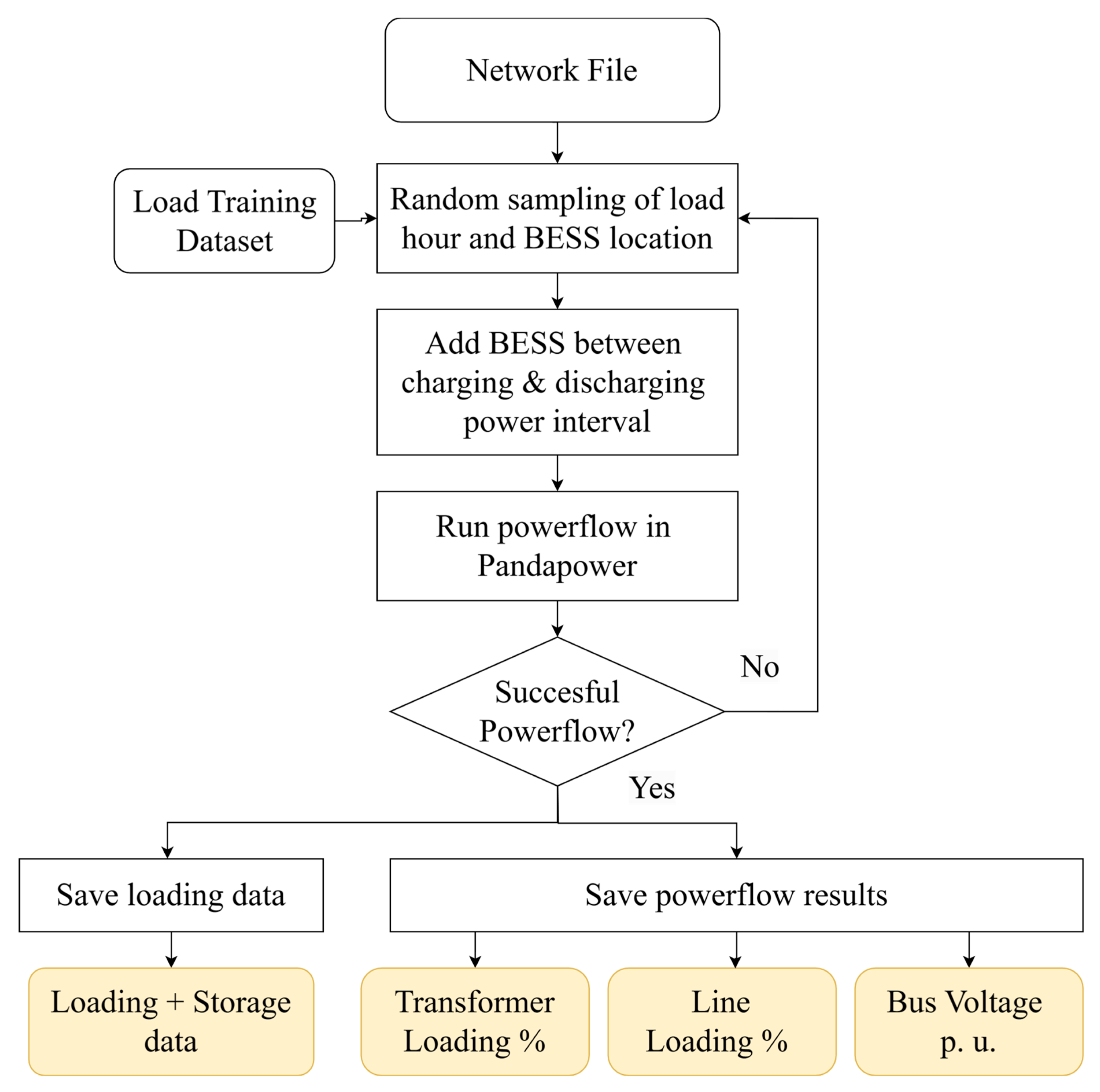
The second phase deals with the creation of synthetic data through power flows using the training dataset of loading data. The DER locations are chosen through randomly sampling buses defined in phase one based on uniform distribution. This was performed since it is seen that random, multiple allocation can help prevent overfitting [48] and is the key method used in our approach to introduce changes to the grid topology. Uniformly randomizing BESS size (±0.5 MW) and location enables each model to generalize across operating scenes without overfitting, providing a simpler alternative to switch-based topology variation, as demonstrated in other works [42]. An overview of this is given in Figure 3.
Load flow analysis was conducted on unique loading and storage scenarios to determine the performance metrics, and the resulting synthetic data was saved in CSV files. This process was repeated iteratively thousands of times, using random sampling of load and storage locations while assuming a specified threshold for both load and storage power values. The transformer loading, line loading, and bus voltage are described in Equations (8)–(10).
Transformer Loading : T , j ( % ) = | S T , j | / S T , j rated × 100
Line Loading : L , m ( % ) = | S L , m | / S L , m rated × 100
Bus Voltage ( p . u . ) : V i ( p . u . ) = V i ( actual ) / V base

2.4. Phase 3: Machine Learning Model Training

The third phase deals with the training of machine learning models for predicting performance metric for each each individual transformer, line, and bus in the network. The training architecture is described in Figure 4. The training data includes the loading and storage scenarios as well as the performance metrics that were generated as the results from power flow in phase 2.
Each scenario n is defined by the active power demand at each low-voltage (LV) bus and the active power injection or consumption from battery energy storage systems (BESSs) across the network. Let P load , k ( n ) denote the load demand at LV bus k and P bess , k ( n ) denote the BESS power at bus k, where P bess , k ( n ) < 0 corresponds to discharging and P bess , k ( n ) > 0 to charging. Using these variables, we can describe the input for scenario n in Equation (11).
x ( n ) = P load , 1 ( n ) , , P load , N load ( n ) , P bess , 1 ( n ) , , P bess , N bess ( n ) ,
where N load is the number of LV loads and N bess is the number of possible BESS injection points. Using the input vector x ( n ) , the desired output is the set of performance metrics computed using pandapower. This includes actual transformer loading percentages, actual line loading percentages, and actual bus voltage magnitudes. The output vector is defined in Equation (12), where T , j ( n ) is the transformer loading percentage for transformer j in scenario n, L , m ( n ) is the line loading percentage for line m in scenario n, V i ( n ) is the voltage magnitude at bus i in scenario n (in p.u.), and N T , N L , and N V denote the number of transformers, lines, and buses, respectively.
z ( n ) = T , 1 ( n ) , , T , N T ( n ) , L , 1 ( n ) , , L , N L ( n ) , V 1 ( n ) , , V N V ( n ) ,
Using the input vector x ( n ) and output vector z ( n ) , a separate machine learning (ML) model is trained for each individual output variable (i.e., a unique model for each line, bus, or transformer). This is achieved by learning a parameterized function f ( x ( n ) ; θ ) that approximates the mapping x y by minimizing a suitable loss function over the dataset. The general training objective is given in Equation (13), where θ represents the trainable parameters of the model (e.g., weights and biases), f ( x ( n ) ; θ ) is the model’s prediction given input vector x ( n ) for scenario n, L ( · , · ) is a loss function measuring the discrepancy between the predicted and true output (e.g., mean squared error), y is either the line loading l L , m ( n ) , transformer loading l T , j ( n ) , or bus voltage V i ( n ) for a specific line, transformer or bus in a specific scenario, and N is the total number of training examples.
θ * = arg min θ 1 N n = 1 N L f ( x ( n ) ; θ ) , y ( n ) ,

2.5. Phase 4: Testing Machine Learning Models

In phase 4, the machine learning models were tested using the testing dataset that was generated in phase 1. The load flow results using this testing dataset are compared with predicted outputs from the ML models that take these loading and storage conditions as inputs. The process for this phase is depicted in Figure 5.
Once a machine learning model f j (e.g., an XGBoost regressor or a neural network) has been trained to predict a specific grid performance metric such as transformer loading T , j , line loading L , m , or bus voltage V i , the inference for a new scenario can be performed directly. Given a new input vector x * , representing updated load demands and BESS setpoints, the predicted output is expressed in Equation (14), where y ^ * is the predicted value of the target variable (e.g., loading percentage or voltage magnitude) for that scenario.
y ^ * = f j ( x * ) ,
This study employs three performance metrics, RMSE, MAE, and MSE to assess predictive accuracy and efficiency. To assess the computational efficiency of the ML models, the speed-up factor is used. It is defined as the ratio of the time required by traditional power flow simulation to the time required for machine learning inference, expressed in Equation (15).
Speed - Up Factor = Time taken by conventional power flow Time taken by ML inference .
A higher speed-up factor indicates a more computationally efficient approach, which is particularly important for real-time or large-scale scenario analysis.

2.6. Selection of Machine Learning Models

XGBoost is an open-source machine learning library [49] designed for efficient and scalable implementation of gradient boosting algorithms. These models are widely used in classification and regression problems for their high speed and satisfactory accuracy. ANNs are computational models inspired by the structure and function of the human brain [50], consisting of interconnected nodes called neurons organized in layers. Each neuron processes input data and passes the result to the next layer through weighted connections, adjusting these weights based on errors using algorithms like backpropagation during training. In this paper, we used Keras [51], an open-source, high-level neural network library in Python, to create a sequential neural network. This paper does not discuss the theory behind these ML models in detail. For a comprehensive understanding, refer to the work cited in this section [49,50,51].

3. Case Study

3.1. Reference Grid

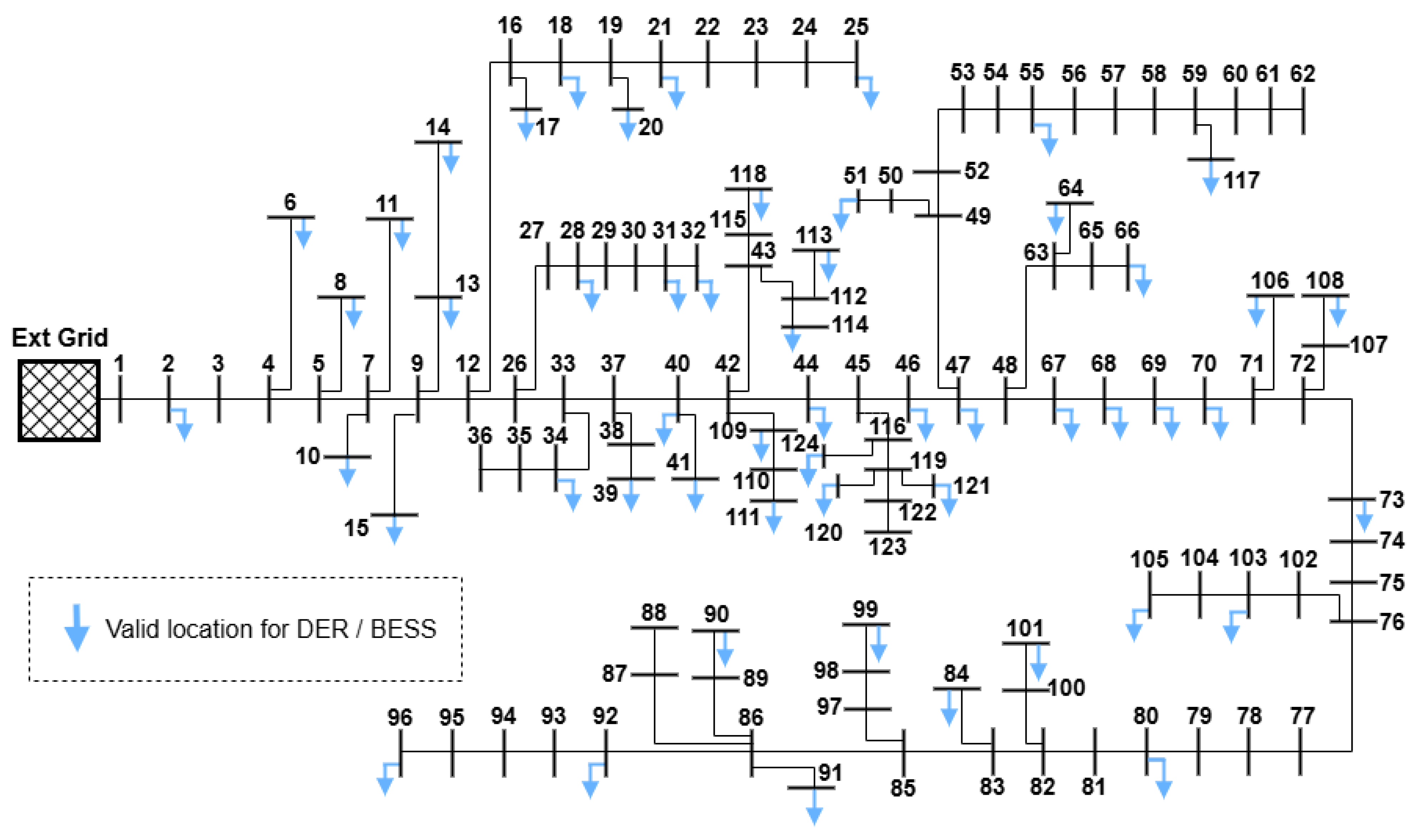
The data for this case study was provided by the Centre for Intelligent Electricity Distribution (CINELDI) [52], a Norwegian research initiative focused on smart grid technologies. They conduct research on grid flexibility, renewable energy integration, digitalization, and cybersecurity. We utilized CINELDI’s Medium Voltage reference grid dataset [53] which is a reference grid that has previously been used for congestion forecasting using probabilistic power flow [54]. The network comprises 185 buses (124 medium voltage + 61 low voltage), 61 transformers, and 122 lines, offering a realistic yet manageable simulation of real-world conditions suitable for our research scope. Figure 6 illustrates this reference grid with all lines indicated. Loads were placed at the low-voltage side of each of the 61 transformers. The loading data, reflective of the conditions in 2018, was also included in the dataset.

3.2. Experimental Parameters

The CINELDI dataset contains 8760 hourly loading values, each treated as an independent scenario. Training data was generated by randomly sampling 500, 1000, 2500, 5000, or 10,000 h. For the 10,000-h case, some timestamps were repeated due to resampling. To simulate BESS integration, low voltage buses were randomly selected for each scenario following a uniform distribution. Each BESS unit was assigned a power range from −0.5 MW (discharging) to 0.5 MW (charging), these values are based on the largest load value seen in the entire dataset of around 0.47 MW. These storage parameters would, in the real world, be appropriate for small residential loads or larger buildings with EVs. A unique BESS setup was defined per hour, with one or more units added based on the desired test configuration. All selected hours were compiled into a single CSV file—each row representing a scenario, with columns indicating load and BESS parameters. A 100% state of charge was assumed for all BESS units. As is frequently done, the dataset was split 80/20 into training and testing sets. During both phases, power flow analysis was conducted for each scenario to compute performance metrics, and results were stored.

Machine Learning Model Details

Multiple machine learning models were trained—one per transformer, line, or bus—to predict loading conditions. For each model type (XGBoost and neural network) and each scenario count (500, 1000, 2500, 5000, and 10,000), this yielded 61 transformer models, 122 line models and 185 bus models. The initial experiments used the MV reference grid with a single BESS per scenario (random size and placement); later scenarios featured multiple randomly sized placed BESS units. Hyperparameters were held constant across all models (see Table 2). A very limited, non-algorithmic grid search based on ranges drawn from prior work and constrained to low values by device compute limits and time was performed, but its results were omitted from this manuscript. Given the hundreds of models trained (around 185 bus, 122 line, 61 transformer × 2 model types), this search was necessarily shallow. We therefore recommend a more comprehensive tuning campaign on more powerful hardware as future work.

4. Results

4.1. Predicting Grid Performance with a Single BESS

Training time is a key factor in evaluating the practicality of ML models. It depends on both the number of training scenarios and the model type. XGBoost is known to train significantly faster than neural networks, a trend confirmed by our results. As shown in Figure 7a, neural network training time is roughly an order of magnitude greater. With 10,000 scenarios, training neural networks can take 4–5 h. Since our goal is to outperform traditional power flow tools, model prediction time must be compared against that of pandapower. Figure 7b highlights the stark contrast: XGBoost delivers predictions far faster than both neural networks and pandapower. For bus voltage, neural networks are even slower than traditional methods.

4.2. Distribution of Mean Square Errors for All Models with a Single BESS

Overall model performance showed that mean square error (MSE) was seen to be lower for ANNs when predicting transformer loading and line loading but higher than XGBoost when predicting bus voltages. Figure 8 presents the MSE distribution for models trained with 10,000 scenarios.

4.3. Predicting Grid Performance with Multiple BESSs

The simulation was repeated for a grid with multiple BESSs installed and the training time was measured for all different scenarios as shown in Figure 9a. Clearly, the training time for neural networks is an order of magnitude higher than for XGBoost models. The prediction time was also measured for all different scenarios. As shown in Figure 9b, again XGBoost significantly outperformed both neural networks and pandapower, except for bus voltage predictions. The overall MSE for each scenario was compared and is shown in Figure 10, where it is evident that ANNs benefit greatly from an increase in the number of training scenarios, whereas XGBoost performs roughly the same even as the number of training scenarios increases.
The distribution of MSE across all these models was assessed. Figure 10 illustrates the distribution of MSE for the various machine learning models trained to predict different performance metrics using 10,000 scenarios for multiple BESSs.
Clearly, ANNs perform significantly better than XGBoost in predicting all performance metrics.

4.4. Compilation of Results

In Table 3, we present the average error metrics and speed-up factors for all the model archetypes in predicting selected grid performance parameters. This table only presents the best-performing models, i.e., with 10,000 training scenarios used for training the models.
The MSE across all models ranges between 0% and 8.09%, reflecting generally good performance, particularly in single-storage injection scenarios. The highest errors are observed with the XGBoost model for multiple-storage cases. For single-storage injections, ANNs outperform XGBoost by achieving an approximately significantly lower MSE and RMSE when predicting transformer loading percentage. However, the difference between these models becomes negligible for predictions of bus voltage (p.u.) and line loading percentage. In multiple-storage scenarios, ANNs demonstrate a marked advantage, with a 56% lower MSE and significantly reduced RMSE compared to XGBoost when predicting transformer loading percentage. Furthermore, ANNs maintain nearly negligible errors for bus voltage (p.u.) and line loading percentage predictions, whereas XGBoost shows starkly higher MSE values. However, for bus voltage (p.u.), XGBoost’s MSE increases only slightly compared to single-storage cases, highlighting some robustness in specific predictions.

5. Discussion

5.1. Inspection of Individual Models

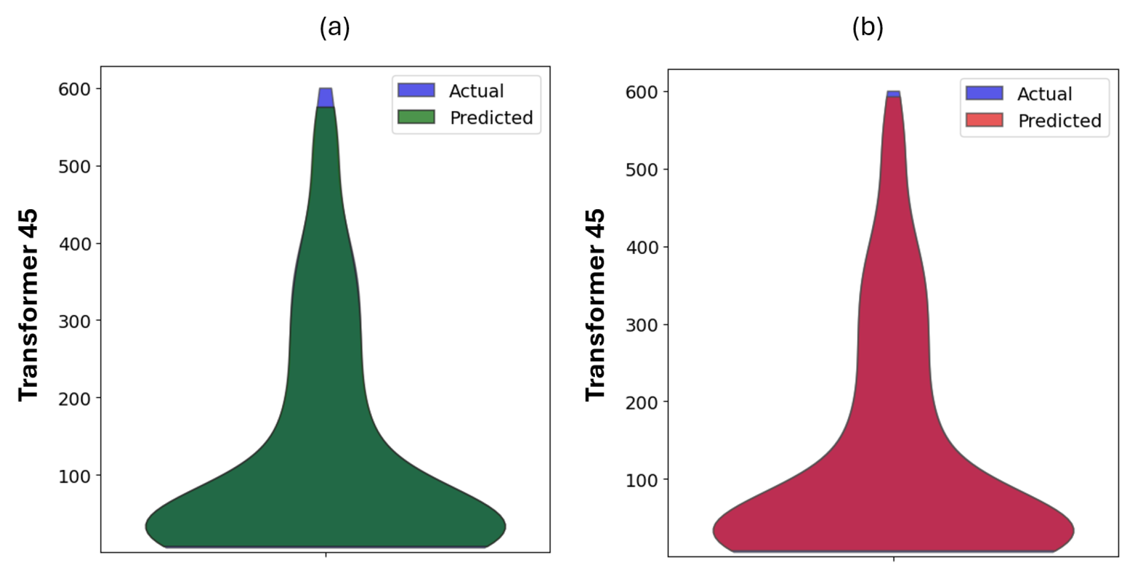
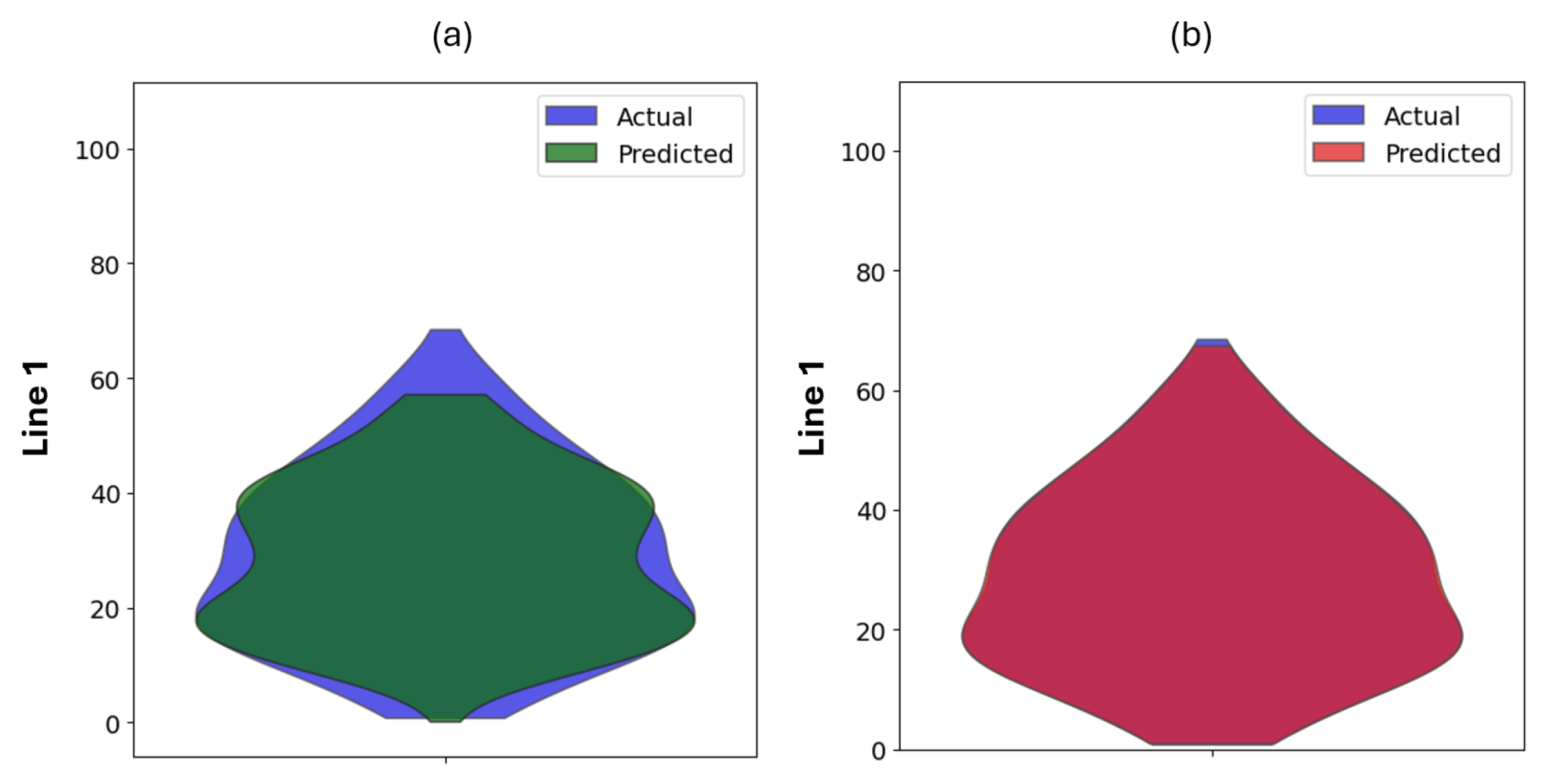
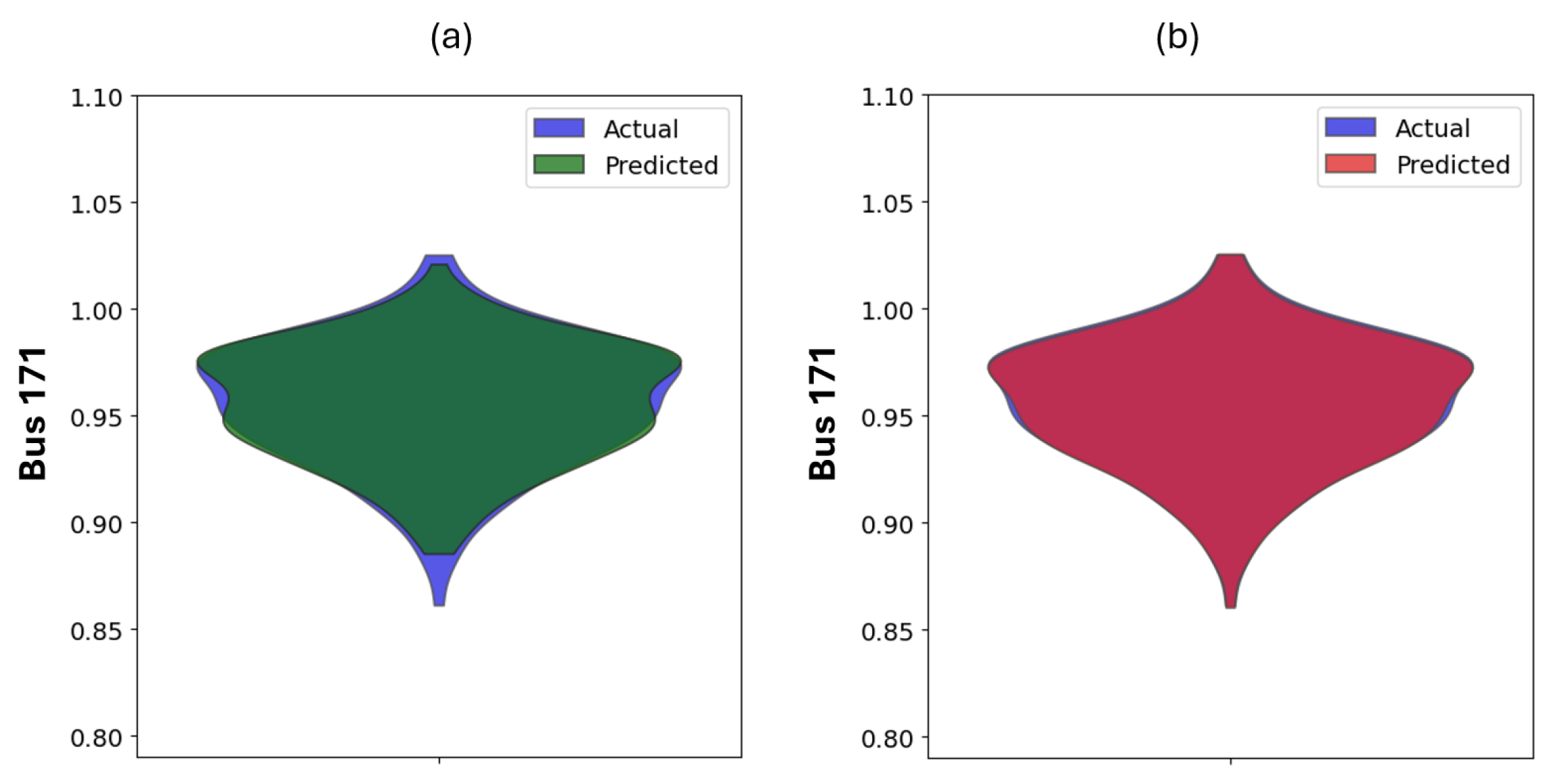
It is also interesting to note that there is a non-insignificant amount of variation in the accuracy of models for each energy storage archetype and for models predicting each performance metric. In the violin charts presented in Figure 11, Figure 12 and Figure 13, the distribution of predicted loading percentages using the testing dataset (200 h) is compared with the actual loading percentages. The extent of overlap indicates the accuracy of the model.
Comparing both models shows that neural network predictions align more closely with actual results than XGBoost, supporting earlier findings that ANNs are generally more accurate. This trend holds across most buses, lines, and transformers. However, for transformer loading percentages, both models perform similarly, with no significant difference in accuracy.

5.2. Comparison Against Traditional Power Flow

To evaluate ML as a viable alternative to traditional power flow, we measured the speed-up factors offered by ML models. As shown in Table 3, these range from 0.89, indicating slightly slower performance, to 45.85, showing significant improvement. XGBoost consistently outperforms ANNs in speed. While average errors for both models remain within acceptable limits, maximum errors can reach 16.49% for XGBoost when predicting transformer loading, which is critical for edge cases while maximum errors remains fairly low for ANNs, making it better suited for predicting the power flow results of edge cases.

6. Conclusions

6.1. Technical Results

This paper introduces a framework using supervised learning models to rapidly solve power flow problems given one or more BESS injection points in an MV distribution network. Unlike prior monolithic surrogates, we train individual models for each component and state variable (185 bus, 122 line, and 61 transformer models per algorithm), which provides fine-grained accuracy insights at the expense of longer training times. By uniformly randomizing BESS size (±0.5 MW) and location across scenarios, a single ANN generalizes to varying topology changes without overfitting, offering a simpler alternative to switch-based methods. We report MAE, MSE, RMSE, maximum error, and speed-up factors to ensure full transparency in edge-case performance that was absent in previous work. In our case study, XGBoost trains up to 100× faster than ANNs and delivers 10–20× prediction speed-ups, while ANNs achieve better accuracy (near 1 % error) and scale favorably with more training scenarios, with significantly lower maximum errors, making them better suited for critical scenarios or edge cases. Overall, ML-based surrogates run up to 10× faster than traditional pandapower analyses while maintaining sub-1 % errors for most state parameters, highlighting their promise for real-time grid planning and operational decision-making. Hence, this study establishes that a single-component–single-model strategy is feasible and transparent, although costlier in training time than monolithic surrogates. Together these findings differentiate our work from meta-learning approaches and multi-topology surrogates.

6.2. Potential Challenges

It is important to emphasize that machine learning-based solutions for grid management and battery operation must be validated using traditional power flow methods and expert oversight to ensure safe and reliable operation. Incorrect or unexpected model predictions could pose operational risks. Additionally, a key limitation of this approach is its sensitivity to parameter changes—such as line outages or transformer reconfigurations—which necessitates retraining the models to accurately reflect the updated network topology.

6.3. Future Work

Future research should leverage high-performance computing resources to reduce training times, as the models in this study were trained using Google Colab’s free compute resources, which significantly limited the performance of the Python environments utilized. Additionally, there is considerable potential for improving model performance through hyperparameter optimization, which was not explored in this paper. While only two types of machine learning models were tested, future studies could explore other model types as well. Furthermore, we plan to benchmark against additional mainstream algorithms (e.g., random forest and LSTM) and classical OPF methods (e.g., fast decoupled power flow) under identical scenarios; although preliminary random forest tests showed inferior performance relative to XGBoost and ANNs, a more systematic comparison will be conducted in future work. In the future, meta-learning techniques can be experimented with to reduce the training time and also attempt training single models for all performance metrics instead of having individual models for each electrical element in the grid.
Future research could use algorithms to modulate the charging and discharging of BESS units to test optimal battery sizes to improve grid performance and use real-time BESS datasets and capacities. Moreover, this study focused on a single open-source dataset, but future work could experiment with more datasets [55,56,57] to understand how models perform with more dynamic or larger networks and to make the solutions more robust, allowing them to handle different topologies. Future work can also benchmark random forest, LSTM, and classical fast-decoupled power-flow methods under identical scenarios.

Author Contributions

Conceptualization, P.Y.; methodology, P.Y. and A.E.S.-G.; simulations, P.Y.; data validation, S.B.-M.; writing—original draft preparation, P.Y.; writing—review and editing, A.E.S.-G., S.B.-M., and M.A.-P.; supervision, A.E.S.-G. and M.A.-P. All authors have read and agreed to the published version of the manuscript.

Funding

This work was funded by the European Union (NextGenerationEU) and the Ministry for Digital Transformation and Public Administration, under the UNICO I + D Cloud call (Grant No. TSI-063100-2022-010), corresponding to the project “Federated Machine Learning for Electrical Distribution Networks” at the Polytechnic University of Catalonia.

Data Availability Statement

The original data presented in the study are openly available on CINELDI’s website.

Conflicts of Interest

The authors declare no conflicts of interest.

References

  1. IEA. Global Installed Grid-Scale Battery Storage Capacity in the Net Zero Scenario, 2015–2030. Available online: https://www.iea.org/data-and-statistics/charts/global-installed-grid-scale-battery-storage-capacity-in-the-net-zero-scenario-2015-2030 (accessed on 5 August 2025).
  2. International Energy Agency. Unlocking the Potential of Distributed Energy Resources; IEA: Paris, France, 2022; Available online: https://www.iea.org/reports/unlocking-the-potential-of-distributed-energy-resources (accessed on 5 August 2025).
  3. Ramos, A.F.; Ahmad, I.; Habibi, D.; Mahmoud, T.S. Placement and sizing of utility-size battery energy storage systems to improve the stability of weak grids. Int. J. Electr. Power Energy Syst. 2023, 144, 108427. [Google Scholar] [CrossRef]
  4. Datta, U.; Kalam, A.; Shi, J. Smart control of BESS in PV integrated EV charging station for reducing transformer overloading and providing battery-to-grid service. J. Energy Storage 2020, 28, 101224. [Google Scholar] [CrossRef]
  5. Wei, R.; Chen, Z.; Wang, Q.; Duan, Y.; Wang, H.; Jiang, F.; Liu, D.; Wang, X. A Mechanical Fault Diagnosis Method for On-Load Tap Changers Based on GOA-Optimized FMD and Transformer. Energies 2025, 18, 3848. [Google Scholar] [CrossRef]
  6. Del Rosso, A.D.; Eckroad, S.W. Energy Storage for Relief of Transmission Congestion. IEEE Trans. Smart Grid 2014, 5, 1138–1146. [Google Scholar] [CrossRef]
  7. Thurner, L.; Scheidler, A.; Schäfer, F.; Menke, J.-H.; Dollichon, J.; Meier, F.; Meinecke, S.; Braun, M. Pandapower—An Open-Source Python Tool for Convenient Modeling, Analysis, and Optimization of Electric Power Systems. IEEE Trans. Power Syst. 2018, 33, 6510–6521. [Google Scholar] [CrossRef]
  8. Gonzalez-Longatt, F.M.; Rueda, J.L. PowerFactory applications for power system analysis. In PowerFactory Applications for Power System Analysis; Springer: Berlin/Heidelberg, Germany, 2014. [Google Scholar] [CrossRef]
  9. Zhang, D.; Li, S.; Zeng, P.; Zang, C. Optimal Microgrid Control and Power-Flow Study with Different Bidding Policies by Using PowerWorld Simulator. IEEE Trans. Sustain. Energy 2014, 5, 282–292. [Google Scholar] [CrossRef]
  10. Cetinay, H.; Soltan, S.; Kuipers, F.A.; Zussman, G.; Van Mieghem, P. Analyzing Cascading Failures in Power Grids under the AC and DC Power Flow Models. SIGMETRICS Perform. Eval. Rev. 2018, 45, 198–203. [Google Scholar] [CrossRef]
  11. Ding, L.; Bao, Z. Analysis on the Self-Organized Critical State with Power Flow Entropy in Power Grids. In Proceedings of the 2009 Second International Conference on Intelligent Computation Technology and Automation, Changsha, China, 10–11 October 2009; IEEE: Changsha, China, 2009; Volume 3, pp. 18–21. [Google Scholar] [CrossRef]
  12. Lukashevich, A.; Maximov, Y. Power Grid Reliability Estimation via Adaptive Importance Sampling. IEEE Control Syst. Lett. 2022, 6, 1010–1015. [Google Scholar] [CrossRef]
  13. Dagle, J. System Operations, Power Flow and Control; PNNL-SA-125328; Pacific Northwest National Laboratory, U.S. Department of Energy: Arlington, VA, USA, 2017. [Google Scholar]
  14. Chow, J.H.; Sanchez-Gasca, J.J. Steady-State Power Flow. In Power System Modeling, Computation, and Control; John Wiley & Sons, Ltd.: Hoboken, NJ, USA, 2019; pp. 9–46. [Google Scholar] [CrossRef]
  15. Čepin, M. Methods for Power Flow Analysis. In Assessment of Power System Reliability: Methods and Applications; Čepin, M., Ed.; Springer: London, UK, 2011; pp. 141–168. [Google Scholar] [CrossRef]
  16. Grainger, J.J.; Stevenson, W.D. Power Flow Analysis. In Power System Analysis; McGraw-Hill: New York, NY, USA, 1994; pp. 330–355. [Google Scholar]
  17. Zimmerman, R.D.; Murillo-Sánchez, C.E.; Thomas, R.J. MATPOWER: Steady-State Operations, Planning, and Analysis Tools for Power Systems Research and Education. IEEE Trans. Power Syst. 2012, 26, 12–19. [Google Scholar] [CrossRef]
  18. About Pandapower. Available online: https://www.pandapower.org/about/ (accessed on 5 August 2025).
  19. Frank, S.; Steponavice, I.; Rebennack, S. Optimal power flow: A bibliographic survey I. Energy Syst. 2012, 3, 221–258. [Google Scholar] [CrossRef]
  20. Azmy, A.M. Optimal Power Flow to Manage Voltage Profiles in Interconnected Networks Using Expert Systems. IEEE Trans. Power Syst. 2007, 22, 1622–1628. [Google Scholar] [CrossRef]
  21. Rau, N. Issues in the path toward an RTO and standard markets. IEEE Trans. Power Syst. 2003, 18, 435–443. [Google Scholar] [CrossRef]
  22. Barja-Martinez, S.; Aragüés-Peñalba, M.; Munné-Collado, Í.; Lloret-Gallego, P.; Bullich-Massagué, E.; Villafafila-Robles, R. Artificial intelligence techniques for enabling Big Data services in distribution networks: A review. Renew. Sustain. Energy Rev. 2021, 150, 111459. [Google Scholar] [CrossRef]
  23. Lu, D.; Hu, D.; Wang, J.; Wei, W.; Zhang, X. A Data-Driven Vehicle Speed Prediction Transfer Learning Method with Improved Adaptability across Working Conditions for Intelligent Fuel Cell Vehicle. IEEE Trans. Intell. Transp. Syst. 2025, 26, 10881–10891. [Google Scholar] [CrossRef]
  24. Utama, C.; Meske, C.; Schneider, J.; Ulbrich, C. Reactive power control in photovoltaic systems through (explainable) artificial intelligence. Appl. Energy 2022, 328, 120004. [Google Scholar] [CrossRef]
  25. Crozier, C.; Baker, K. Data-Driven Probabilistic Constraint Elimination for Accelerated Optimal Power Flow. In Proceedings of the 2022 IEEE Power & Energy Society General Meeting (PESGM), Denver, CO, USA, 17–21 July 2022; IEEE: Denver, CO, USA, 2022; pp. 1–5. [Google Scholar] [CrossRef]
  26. Hasan, F.; Kargarian, A.; Mohammadi, A. A Survey on Applications of Machine Learning for Optimal Power Flow. In Proceedings of the 2020 IEEE Texas Power and Energy Conference (TPEC), College Station, TX, USA, 6–7 February 2020; IEEE: College Station, TX, USA, 2020; pp. 1–6. [Google Scholar] [CrossRef]
  27. Saldaña-González, A.E.; Aragüés-Peñalba, M.; Sumper, A. Distribution network planning method: Integration of a recurrent neural network model for the prediction of scenarios. Electr. Power Syst. Res. 2024, 229, 110125. [Google Scholar] [CrossRef]
  28. Bernadić, A.; Kujundžić, G.; Primorac, I. Reinforcement Learning in Power System Control and Optimization. B&H Electr. Eng. 2023, 17, 26–34. [Google Scholar] [CrossRef]
  29. Guha, N.; Wang, Z.; Wytock, M.; Majumdar, A. Machine Learning for AC Optimal Power Flow. arXiv 2019. [Google Scholar] [CrossRef]
  30. Lei, X.; Yang, Z.; Yu, J.; Zhao, J.; Gao, Q.; Yu, H. Data-Driven Optimal Power Flow: A Physics-Informed Machine Learning Approach. IEEE Trans. Power Syst. 2021, 36, 346–354. [Google Scholar] [CrossRef]
  31. Nellikkath, R.; Chatzivasileiadis, S. Physics-Informed Neural Networks for AC Optimal Power Flow. Electr. Power Syst. Res. 2022, 212, 108412. [Google Scholar] [CrossRef]
  32. Pagnier, L.; Chertkov, M. Physics-Informed Graphical Neural Network for Parameter & State Estimations in Power Systems. arXiv 2021. [Google Scholar] [CrossRef]
  33. Li, Y.; Zhao, C.; Liu, C. Model-Informed Generative Adversarial Network for Learning Optimal Power Flow. IISE Trans. 2024, 57, 30–43. [Google Scholar] [CrossRef]
  34. Zhen, H.; Zhai, H.; Ma, W.; Zhao, L.; Weng, Y.; Xu, Y.; Shi, J.; He, X. Design and Tests of Reinforcement-Learning-Based Optimal Power Flow Solution Generator. Energy Rep. 2022, 8 (Suppl. 1), 43–50. [Google Scholar] [CrossRef]
  35. Pu, T.; Wang, X.; Cao, Y.; Liu, Z.; Qiu, C.; Qiao, J.; Zhang, S. Power flow adjustment for smart microgrid based on edge computing and multi-agent deep reinforcement learning. J. Cloud Comput. 2021, 10, 48. [Google Scholar] [CrossRef]
  36. Balduin, S.; Tröschel, M.; Lehnhoff, S. Towards domain-specific surrogate models for smart grid co-simulation. Energy Inform. 2019, 2, 27. [Google Scholar] [CrossRef]
  37. Junior, J.; Pinto, T.; Morais, H. Hybrid classification-regression metric for the prediction of constraint violations in distribution networks. Electr. Power Syst. Res. 2023, 221, 109401. [Google Scholar] [CrossRef]
  38. Balduin, S.; Westermann, T.; Puiutta, E. Evaluating different machine learning techniques as surrogate for low voltage grids. Energy Inform. 2020, 3, 24. [Google Scholar] [CrossRef]
  39. Yang, Y.; Yang, Z.; Yu, J.; Zhang, B.; Zhang, Y.; Yu, H. Fast Calculation of Probabilistic Power Flow: A Model-Based Deep Learning Approach. IEEE Trans. Smart Grid 2020, 11, 2235–2244. [Google Scholar] [CrossRef]
  40. Li, S.; Pan, Z.; Li, H.; Xiao, Y.; Liu, M.; Wang, X. Convergence criterion of power flow calculation based on graph neural network. J. Phys. Conf. Ser. 2024, 2703, 012042. [Google Scholar] [CrossRef]
  41. Chen, Y.; Lakshminarayana, S.; Maple, C.; Poor, H.V. A Meta-Learning Approach to the Optimal Power Flow Problem Under Topology Reconfigurations. arXiv 2021. [Google Scholar] [CrossRef]
  42. Menke, J.-H.; Bornhorst, N.; Braun, M. Distribution System Monitoring for Smart Power Grids with Distributed Generation Using Artificial Neural Networks. arXiv 2019. [Google Scholar] [CrossRef]
  43. Zamzam, A.; Baker, K. Learning Optimal Solutions for Extremely Fast AC Optimal Power Flow. arXiv 2019, arXiv:1910.01213. [Google Scholar] [CrossRef]
  44. Talebi, S.; Zhou, K. Graph Neural Networks for Efficient AC Power Flow Prediction in Power Grids. arXiv 2025, arXiv:2502.05702. [Google Scholar]
  45. Jadhav, S.; Sevak, B.; Das, S.; Su, W.; Bui, V.-H. Enhancing Power Flow Estimation with Topology-Aware Gated Graph Neural Networks. arXiv 2025, arXiv:2507.02078. [Google Scholar] [CrossRef]
  46. Xia, X.; Xiao, L.; Ye, H. Deep Learning-Based Correlation Analysis for Probabilistic Power Flow Considering Renewable Energy and Energy Storage. Front. Energy Res. 2024, 12, 1365885. [Google Scholar] [CrossRef]
  47. Menke, J.-H.; Dipp, M.; Liu, Z.; Ma, C.; Schäfer, F.; Braun, M. Applications of Artificial Neural Networks in the Context of Power Systems. In Artificial Intelligence Techniques for a Scalable Energy Transition: Advanced Methods, Digital Technologies, Decision Support Tools, and Applications; Springer International Publishing: Cham, Switzerland, 2020; pp. 345–373. [Google Scholar] [CrossRef]
  48. Jia, J.; Yuan, S.; Shi, Y.; Wen, J.; Pang, X.; Zeng, J. Improved Sparrow Search Algorithm Optimization Deep Extreme Learning Machine for Lithium-Ion Battery State-of-Health Prediction. iScience 2022, 25, 103988. [Google Scholar] [CrossRef]
  49. Chen, T.; Guestrin, C. XGBoost: A Scalable Tree Boosting System. In Proceedings of the 22nd ACM SIGKDD International Conference on Knowledge Discovery and Data Mining, San Francisco, CA, USA, 13–17 August 2016; ACM: New York, NY, USA, 2016; pp. 785–794. [Google Scholar] [CrossRef]
  50. Jain, A.K.; Mao, J.; Mohiuddin, K.M. Artificial neural networks: A tutorial. Computer 1996, 29, 31–44. [Google Scholar] [CrossRef]
  51. Watson, M.; Chollet, F.; Sreepathihalli, D.; Saadat, S.; Sampath, R.; Rasskin, G.; Zhu, S.; Singh, V.; Wood, L.; Tan, Z.; et al. Keras. Available online: https://keras.io (accessed on 5 August 2025).
  52. Centre for Intelligent Electricity Distribution. Available online: https://www.sintef.no/projectweb/cineldi/ (accessed on 5 August 2025).
  53. Sperstad, I.B.; Fosso, O.B.; Jakobsen, S.H.; Eggen, A.O.; Evenstuen, J.H.; Kjølle, G. Reference data set for a Norwegian medium voltage power distribution system [dataset]. Data Brief 2023, 47, 109025. [Google Scholar] [CrossRef] [PubMed]
  54. Hernandez-Matheus, A.; Berg, K.; Gadelha, V.; Aragüés-Peñalba, M.; Bullich-Massagué, E.; Galceran-Arellano, S. Congestion forecast framework based on probabilistic power flow and machine learning for smart distribution grids. Int. J. Electr. Power Energy Syst. 2024, 156, 109695. [Google Scholar] [CrossRef]
  55. Kazmi, H.; Munné-Collado, Í.; Mehmood, F.; Syed, T.A.; Driesen, J. Towards data-driven energy communities: A review of open-source datasets, models and tools. Renew. Sustain. Energy Rev. 2021, 148, 111290. [Google Scholar] [CrossRef]
  56. Athay, T.; Podmore, R.; Virmani, S. A Practical Method for the Direct Analysis of Transient Stability. IEEE Trans. Power Appar. Syst. 1979, PAS-98, 573–584. [Google Scholar] [CrossRef]
  57. Peña, I.; Martinez-Anido, C.B.; Hodge, B.-M. An Extended IEEE 118-Bus Test System with High Renewable Penetration. IEEE Trans. Power Syst. 2018, 33, 281–289. [Google Scholar] [CrossRef]
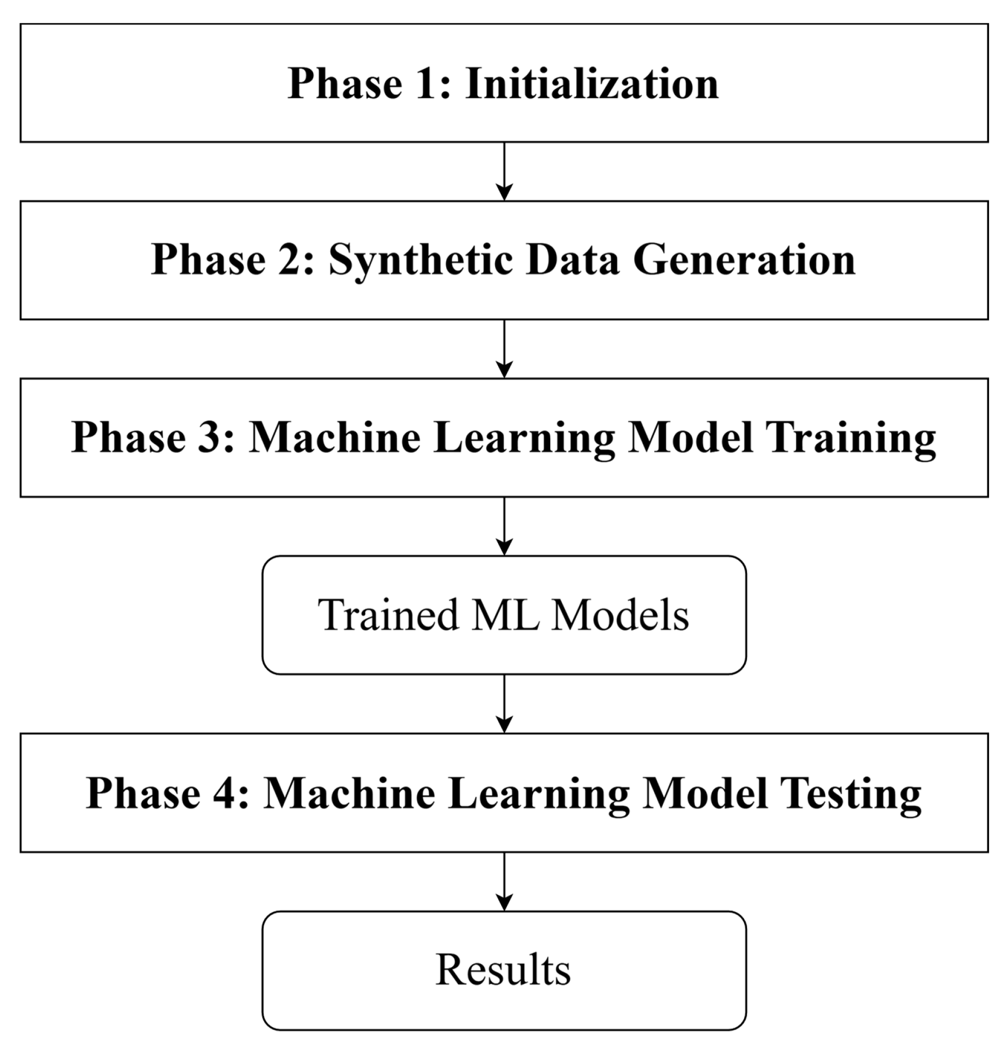
Figure 1. Overview of the overall methodology. The entire process is split into four key phases, similar to most ML training and testing exercises.
Energies 18 04416 g001
Figure 2. Initialization of the relevant network files from real-world data required for generating synthetic data.
Energies 18 04416 g002
Figure 3. Steps taken during the synthetic data generation phase, which would later be used for training and testing the ML models.
Energies 18 04416 g003
Figure 4. Training of ML models using previously generated data, including grid performance metrics, loading, and storage data.
Energies 18 04416 g004
Figure 5. Actions taken during the testing of ML models, with results being saved from predictions and actual power flow calculations. Metric errors such as MAE, MSE, RMSE, and max errors are calculated.
Energies 18 04416 g005
Figure 6. CINELDI’s Medium Voltage reference grid, with all lines indicated. Blue arrows indicate valid locations for DERs/BESSs and were used by the algorithm for DER placement. Numbers represent the line number that connect to MV buses; LV buses and transformers not shown in this representation.
Energies 18 04416 g006
Figure 7. (a) Time required for the training of machine learning models and (b) time required for prediction from different ML models using a different number of training scenarios when a single BESS is installed in the grid.
Energies 18 04416 g007
Figure 8. Distribution of MSE for models trained on 10,000 scenarios for a network with a single storage unit: (a) Performance of the 61 transformer loading percent models (b) Performance of the 122 line loading percent models (c) Performance of the 185 bus voltage p.u. models. The boxes indicate the 25th and 75th percentile values, the outliers are presented as dots, which are defined as 1.5 times the interquartile range between the aforementioned percentiles.
Energies 18 04416 g008
Figure 9. (a) Time required for the training of machine learning models and (b) time required for prediction for different ML models using a different number of training scenarios when multiple BESSs are installed in the grid.
Energies 18 04416 g009
Figure 10. Distribution of MSE for models trained on 10,000 scenarios for a network with multiple storage units: (a) Performance of 61 transformer loading percent models (b) Performance of 122 line loading percent models (c) Performance of 185 bus voltage p.u. models. The boxes indicate the 25th and 75th percentile values, the outliers are presented as dots, which are defined as 1.5 times the interquartile range between the aforementioned percentiles.
Energies 18 04416 g010
Figure 11. Distribution of predicted and actual values for transformer loading percent for transformer 45 using 10,000 scenarios with multiple energy storage units for training vs. actual transformer loading percent predicted by (a) XGBoost and (b) ANN models.
Energies 18 04416 g011
Figure 12. Distribution of predicted and actual values for line loading percent for line 1 using 10,000 scenarios with multiple energy storage units for training vs. actual line loading percent predicted by (a) XGBoost and (b) ANN models.
Energies 18 04416 g012
Figure 13. Distribution of predicted and actual values for bus voltage percentage units for bus 171 using 10,000 scenarios with multiple energy storage units for training vs. actual bus voltages predicted by (a) XGBoost and (b) ANN models.
Energies 18 04416 g013
Table 1. Summary of ML-based approaches for OPF: methods, key results, and identified limitations.
LiteratureApproachConclusionDrawbacks/Limitations
[36]Deep Neural Network used to predict bus voltages on the CIGRE LV networkAvg. speed-up factor 2.65; normalized RMSE 7.5%; precision in critical cases 18%Incompatible with critical grid situations; fixed topology only
[37]LR, SVM, SVR, GB, XGBoost, and ANN models to predict bus voltage constraint violationsAccuracy 94–98%; precision 37–52%Incompatible with critical grid situations; fixed topology only; no cross-model comparison
[38]LR, RF, KNN, LSTM, and ANN on CIGRE LV and LV-rural3 networks assessing PV and phase-angle effectsRMSE < 0.001 (LR & ANN best); speed-up factor 0.69–9.5× depending on model/topologyIncompatible with critical grid situations; other state parameters omitted; fixed topology only
[39]DNN to approximate power flow on IEEE test systemsErrors < 8.1%; speed-up factor 1234–2040× depending on topologyIncompatible with critical grid situations; single-topology models only
[40]Graph Neural Network to classify convergence of power flow on the IEEE 14-bus systemAccuracy 99.3%; F1 Score 99.3%Does not compute power flow; only predicts convergence
[41]Meta-learning DNNs pretrained across IEEE 14-, 30-, and 118-bus systems for topology-agnostic initializationAccuracy 97%; pretrained models train faster on new topologiesNo maximum error bounds or critical-case handling; needs many topologies for effective MTL
[42]ANN vs. state estimation using partial measurements in dynamic CIGRE MV network>99% accuracy for ANN with ample measurements; higher errors under sparse measurementsIncompatible with critical grid situations; high errors with minimal measurement sets
[43]DNN to speed up AC OPF calculations on IEEE test systemsSpeed-up factor 6–22×Restricted to single topology; accuracy metrics and training time missing; requires post-processing to retrieve state parameters
[44]Graph Neural Network used to solve AC OPF on various IEEE test systemsNormalized RMSE < 0.05; R2 scores near 1No insight into maximum error or critical-case performance; fixed topology only
[45]Graph Neural Network to solve AC OPF with topology changes on IEEE test systemsRMSE < 0.17; MAE < 0.084; voltage angle error mostly <0.002 radNo reported speed-up metrics; limited variation; training time 7 h for large networks
[46]DNN to predict power flow fluctuations due to energy storage operations on IEEE test systems vs. probabilistic power flowSubstantial speed-up >700× vs. Latin Hypercube Sampling; max error 6.59%Restricted to single topology; storage modeling needs improvement
Table 2. Hyperparameters chosen for training machine learning models based on limited grid-search.
Hyperparameter(s)Value
XGBoost
Loss functionSquared Error
Number of Estimators314
Neural Network
Loss functionSquared Error
Activation functionReLU
Number of layers3
Neurons per layer64, 64, 64
Epochs100
Batch Size32
Table 3. Comparison of the average error metrics and speed up factors for all machine learning models trained on 10,000 scenarios.
Model TypeMSERMSEMAE (%)Max Error (%)Speed-Up Factor
Transformer Loading %
XGBoost Single Storage2.931.40.2616.4945.85
XGBoost Multi Storage7.092.441.5411.5232.96
ANN Single Storage0.810.710.435.432.87
ANN Multi Storage3.131.541.096.893.67
Line Loading %
XGBoost Single Storage0.150.220.131.2227.46
XGBoost Multi Storage8.091.421.044.9538.10
ANN Single Storage00.020.020.121.43
ANN Multi Storage0.050.130.090.692.49
Bus Voltage p.u.
XGBoost Single Storage0.010.080.050.3714.11
XGBoost Multi Storage0.230.440.331.5719.69
ANN Single Storage0.020.10.090.360.89
ANN Multi Storage0.020.140.110.641.24
Disclaimer/Publisher’s Note: The statements, opinions and data contained in all publications are solely those of the individual author(s) and contributor(s) and not of MDPI and/or the editor(s). MDPI and/or the editor(s) disclaim responsibility for any injury to people or property resulting from any ideas, methods, instructions or products referred to in the content.