Oil Futures Dynamics and Energy Transition: Evidence from Macroeconomic and Energy Market Linkages

Abstract

Understanding the price dynamics of oil futures is crucial for advancing green finance strategies and supporting sustainable energy transitions. This study investigates the macroeconomic and energy market determinants of oil futures prices through Granger causality, cointegration analysis, and the error correction model, using daily data. It focuses on the influence of economic development levels, exchange rate fluctuations, and inter-energy price linkages. The empirical findings indicate that (1) oil futures prices exhibit strong correlations with other energy prices, macroeconomic factors, and exchange rate variables; (2) economic development significantly affects oil futures prices, while exchange rate impacts are statistically insignificant based on the daily data analyzed; (3) there exists a stable long-term equilibrium relationship between oil futures prices and variables representing economic activity, exchange rates, and energy market trends; (4) oil futures prices exhibit significant short-term dynamics while adjusting steadily toward a long-run equilibrium driven by macroeconomic and energy market fundamentals. By enhancing the accuracy of oil futures price forecasting, this study offers practical insights for managing financial risks associated with fossil energy markets and contributes to the formulation of low-carbon investment strategies. The findings provide a valuable reference for integrating energy pricing models into sustainable finance and climate-aligned portfolio decisions.

1. Introduction

In the face of intensifying climate challenges and mounting energy security concerns, the global energy system is undergoing a profound transformation [1]. Energy transition, characterized by a gradual shift from fossil fuel dependence to cleaner, more sustainable energy sources—has become central to achieving long-term environmental and economic resilience. This transformation is not only technological but also structural and financial, requiring a comprehensive realignment of energy markets, policy frameworks, and industrial models. Within this context, understanding the pricing dynamics of key energy commodities—especially oil—remains essential for anticipating market shifts, managing investment risks, and designing forward-looking energy strategies.

Crude oil, as a cornerstone of the global energy mix, continues to exert far-reaching influence on economic performance, inflation expectations, and financial market stability [2]. Although the transition toward renewable energy is accelerating, oil futures prices remain a critical barometer for global energy market sentiment [3]. They are shaped by complex interactions among macroeconomic conditions, geopolitical risks, and inter-energy market linkages. Recent studies, such as Marquez and Ren [4], have emphasized the role of short-term financial arbitrage and exchange rate dynamics by employing a daily-frequency VAR model to uncover co-movements among oil, gold, and foreign exchange markets. Their findings highlight the empirical challenges posed by market anomalies—such as the 2020 negative oil price event—which necessitate linear alternatives to traditional log-linear formulations. While informative, such approaches primarily focus on short-run asset market relationships. In contrast, this study adopts a broader structural lens, incorporating macroeconomic development indicators, inter-energy price linkages, and long-term cointegration analysis to investigate oil futures pricing mechanisms within the context of the low-carbon transition. Moreover, accurate oil price forecasting has become increasingly important for informing sustainable energy policies, enhancing corporate risk management, and facilitating green financial decision-making [5]. In this context, deeper insights into the determinants and long-term dynamics of oil futures prices can provide valuable support for the strategic reallocation of energy investments and the design of effective transition pathways.

Nevertheless, fossil energy—particularly oil—still constitutes a substantial portion of the global energy structure, especially in emerging and resource-constrained economies. Under this reality, oil price fluctuations exert profound influences not only on energy security and economic stability but also on the cost structure and investment decisions associated with low-carbon transitions [6]. Therefore, strengthening oil price risk management through the development of oil futures markets and prediction technologies becomes an essential strategy [7].

In this regard, participating in international oil futures trading and accelerating the development of domestic oil futures markets are widely regarded as effective short-term responses to mitigate oil price risks [8]. More importantly, developing accurate oil futures price forecasting technologies from a low-carbon economic perspective enables better alignment between market signals and policy objectives [9]. By capturing short-term volatility and long-term trends, predictive models can provide robust decision support for governments and enterprises in balancing economic growth, energy security, and environmental goals. Furthermore, integrating low-carbon indicators—such as carbon intensity, renewable energy investment, or green finance signals—into oil futures pricing models could enhance the market’s capacity to reflect low-carbon transition dynamics.

Thus, oil futures markets not only serve traditional roles in price discovery and risk hedging but also carry growing significance in promoting energy structure optimization, guiding green investment flows, and supporting the transition toward a low-carbon economy [10]. Strengthening their function through predictive analytics and policy coordination is crucial for building a resilient, sustainable energy system that meets the dual objectives of economic stability and environmental responsibility. Figure 1 shows the fluctuation trend of WTI crude oil prices from 1999 to May 2025.

Based on the above observations, this study investigates the formation mechanisms and key determinants of international oil futures prices within the broader context of low-carbon economic transformation and the financialization of energy markets. As a forward-looking market instrument, crude oil futures not only reflect immediate supply-demand conditions but also shape expectations, influence strategic behavior, and signal long-term trends that are critical for guiding the trajectory of energy transitions. In particular, accurate forecasting of oil futures prices can help policymakers anticipate fossil fuel market volatility and manage transition-related risks more proactively. For example, when oil futures indicate a structural decline in long-term prices due to tightening climate policies or declining demand, this provides early signals for governments to reduce fiscal reliance on oil revenues, redesign subsidy frameworks, and accelerate investment in alternative energy infrastructure. Countries like Norway, through its sovereign wealth fund, and the United Arab Emirates, via its energy diversification strategy, have leveraged such price signals to adjust their national energy strategies and reallocate capital toward renewables. Moreover, oil price expectations serve as a coordination mechanism across public and private actors. Lower expected oil prices over time can deter long-term investment in carbon-intensive assets (e.g., new upstream oil projects), thereby reducing the risk of carbon lock-in. Simultaneously, they strengthen the relative attractiveness of low-carbon technologies by shifting the risk-return profile in favor of green innovation. For policymakers, this facilitates more informed timing of carbon pricing, infrastructure rollout, and just transition planning. Therefore, forecasting oil futures prices is not merely a technical forecasting task; it directly informs policy design, fiscal planning, and strategic coordination in the global effort to phase out fossil fuels. It serves as a bridge between market expectations and policy action, enabling governments to steer the energy system toward decarbonization in a more adaptive, transparent, and economically rational manner.

Distinct from existing studies that focus either on physical supply-demand fundamentals or purely financial variables, this paper integrates a cross-domain analytical framework that combines macroeconomic development indicators, energy price linkages, and exchange rate dynamics. The use of Granger causality tests and cointegration analysis is theoretically grounded in the time-series behavior of energy markets, which are characterized by non-stationary, interdependent variables and long-term equilibrium relationships. Granger causality helps capture predictive lead-lag structures, while cointegration analysis uncovers stable, long-run co-movements between oil futures prices and macro-financial variables. These methods are particularly suited to markets with increasing short-term volatility and complex structural dependencies, such as oil futures under energy transition dynamics. The contributions of this study are summarized as follows:

(1) Theoretically-guided identification of drivers and dynamic structures in oil futures pricing. Drawing from energy finance literature and macroeconomic theory, this study clarifies how economic development, energy price substitution effects, and currency valuation interact to shape crude oil futures prices. Notably, the analysis reveals that exchange rate effects, while emphasized in earlier studies, are relatively insignificant compared to energy price linkages, highlighting a potential paradigm shift in energy-finance interactions.

(2) Methodological innovation in energy forecasting under systemic transformation. Although using established econometric tools, this study innovatively applies them within a low-carbon transition context, uncovering temporal asymmetries, structural couplings, and predictive patterns not explored in prior models. The framework provides a replicable, policy-relevant toolkit for forecasting fossil energy prices amid growing renewable competition and geopolitical volatility.

(3) Policy-relevant insights for enhancing futures market resilience. The paper provides recommendations for refining oil futures market architecture—such as improving regulatory coherence, market liquidity, and price signal quality—thus aligning futures trading mechanisms with the evolving goals of carbon neutrality, resource efficiency, and financial stability.

The remainder of this paper is organized as follows: Section 2 is a literature review; Section 3 is data description and methods; Section 4 is a discussion of the research results; and Section 5 is conclusions and recommendations.

2. Literature Review

The accelerating global shift toward cleaner, more sustainable energy systems is fundamentally reshaping the structure and dynamics of energy markets [11]. Within this transition, oil futures prices continue to play a pivotal role—not only as indicators of traditional supply-demand fundamentals, but also as forward-looking signals that can shape long-term investment, production, and policy trajectories. Crucially, oil futures influence how energy producers, investors, and policymakers perceive and respond to transition-related risks, including the prospect of stranded assets, capital misallocation, and fossil fuel price volatility. For policymakers specifically, oil futures serve as both a barometer and a compass. On one hand, they reflect market expectations about the viability and cost-competitiveness of fossil fuels, sending signals about the urgency and feasibility of decarbonization. On the other hand, accurate forecasts of oil prices allow governments to better anticipate revenue fluctuations, design adaptive fiscal frameworks, and time their phase-out of fossil fuel subsidies more effectively. This improves the credibility and efficiency of policy instruments aimed at accelerating the shift toward renewables, such as carbon pricing, green industrial policies, or energy tax reforms.

Moreover, oil price expectations significantly affect public and private sector investment decisions in energy infrastructure. When future oil prices are forecasted to decline in the context of stronger climate commitments, the perceived economic case for clean energy technologies strengthens—thereby catalyzing a faster reallocation of capital toward low-carbon solutions. This strategic alignment between oil market expectations and policy planning helps reduce lock-in effects, encourages technological innovation, and builds social and economic resilience against fossil fuel dependency. Therefore, understanding and forecasting oil futures is not merely a financial exercise; it is a foundational component of effective energy transition governance. A robust oil price forecasting framework enhances systemic foresight, mitigates transition-related uncertainty, and provides a vital informational bridge between short-term market dynamics and long-term sustainability goals.

2.1. Oil Futures Prices: Cross-Market Impacts and Adaptive Mechanisms

Oil futures prices serve as a pivotal economic indicator that not only reflects the expectations of market participants but also transmits risks and information across energy, financial, and industrial sectors. With increasing geopolitical uncertainties and climate policy transformations, the mechanisms through which oil prices influence and adapt to various markets have attracted growing scholarly interest. Recent studies have explored the dynamic interplay between oil futures prices and variables such as clean energy mineral prices, stock returns, macroeconomic indicators, and investor sentiment, revealing a multi-layered and evolving system of interconnections.

In terms of cross-market linkages between oil prices and clean energy or commodity markets, Jiang et al. [12] employed quantile and wavelet approaches to verify the long-term equilibrium between oil prices and clean energy mineral prices. They found that in stable markets, oil prices significantly affect key minerals such as cobalt, lithium, and rare earths, while in highly volatile markets, such influence becomes negligible. Zhang et al. [13] further revealed dynamic co-movements between oil futures and Chinese agricultural commodity prices using a VECM-CMGARCH model and spatial hypergraph neural network, highlighting oil’s predictive role for agricultural futures. Meanwhile, Oglend and Kleppe [14] constructed a modified storage model with counterfactual analysis, showing that during capacity shortages, inventory rigidity increases oil price uncertainty, thus explaining discrepancies between traditional models and actual market dynamics. Beyond price-based market interactions, Deschryver and De Mariz [15] highlight key institutional barriers to scaling green finance. Based on interviews and market data, they identify the lack of global standards, greenwashing risks, high issuance costs, and limited supply as major constraints in the green bond market. These findings underscore that without robust and scalable financing instruments, such as green bonds, the broader goals of clean energy investment and decarbonization remain difficult to achieve.

In terms of transmission mechanisms to stock markets and macroeconomic activities, Andrikopoulos et al. [16] utilized MIDAS and Granger causality tests to demonstrate that oil prices affect shipping freight rates, which in turn drive stock price volatility—an effect especially pronounced during crises such as COVID-19 and the Russia–Ukraine conflict. Heinlein and Mahadeo [17], using a smooth transition VAR model, found that oil price uncertainty affects U.S. stock markets differently across regimes, with stronger reactions under low uncertainty conditions. From a Chinese perspective, Xu et al. [8] showed that domestic crude oil futures (SC) outperform international oil prices in predicting industrial growth and pricing stock market risks, providing evidence of localized pricing power. Arouri et al. [18] emphasized the role of climate policy uncertainty in weakening the oil-stock return link, with GCC markets showing negative marginal effects under delayed oil price conditions.

In terms of investor behavior and sentiment response to oil price shocks, Li [19] adopted a nonlinear ARDL model and found that both positive and negative oil price shocks enhance U.S. investor sentiment, with negative effects being more persistent and increasingly asymmetric over time. Huang et al. [20] identified a positive correlation between oil price volatility and corporate green innovation disclosure, moderated by environmental performance, legitimacy concerns, and political connections. Cai et al. [21] used generalized forecast error variance decomposition to show that airline stock returns became more sensitive to oil supply and demand shocks post-COVID-19, indicating heightened investor sensitivity to oil price-induced risks.

In terms of oil price volatility as a driver of innovation and strategic response, Huangfu et al. [22] examined the impact of oil price fluctuations on China’s NEV (new energy vehicle) innovation using ARDL and dynamic counterfactual simulation. They found that short-term oil price shocks significantly stimulate NEV innovation, though the long-term inducement weakens. This suggests that volatility, rather than trend level, may be a more critical trigger for strategic technological responses. This insight complements research on adaptive behaviors across industries in response to energy cost uncertainty.

In terms of price–volume relationships and market microstructure, price-volume dynamics remain central to understanding oil futures markets. Xu et al. [23] emphasized that volume reflects investor expectations and supports technical analysis. Empirical studies by Wang et al. [24] and Jena et al. [25] found evidence for volume affecting prices but limited linear causality in fuel oil markets. Go and Lau [26] showed that while no linear causality was observed from price to volume, nonlinear tests revealed bidirectional causality depending on sample period and contract maturity.

The above literature collectively underscores the multifaceted role of oil futures prices as both transmitters and recipients of information in a complex global system. From clean energy commodities to stock markets, from investor sentiment to industrial innovation, oil prices exhibit dynamic, non-linear, and often asymmetric effects. Scholars increasingly adopt advanced models such as wavelet analysis, neural networks, and regime-switching VARs to capture these evolving patterns. Yet, gaps remain in understanding the long-term feedback mechanisms and their policy implications, particularly under extreme events and in emerging markets. Future research should further explore these interactions with a focus on adaptive market behavior, systemic resilience, and low-carbon transition pathways.

2.2. Oil Futures Forecasting: Predictive Innovations and Model Advancements

In the context of accelerating the low-carbon transition and navigating energy market volatility, the accurate forecasting of oil futures prices has become crucial for policymakers, investors, and enterprises. Traditional econometric models are increasingly being supplemented—and sometimes replaced—by hybrid, machine learning, and quantum computing approaches that better accommodate the nonlinearity, regime shifts, and high-frequency characteristics of oil price behavior.

In terms of the integration of quantum computing and deep learning models, Zhai et al. [5] introduced a Quantum Deep Learning framework using Shanghai crude oil futures data combined with multi-market factors. Their results indicate that Quantum Long Short-Term Memory (QLSTM) and Quantum Gate Recurrent Unit (QGRU) models outperform traditional deep learning methods, with performance significantly influenced by quantum gate combinations and qubit settings. These models showed consistent robustness across variable settings, underscoring the potential of quantum-optimized architectures in oil price prediction.

In terms of machine learning algorithms and nonlinear causality, recent studies have leveraged machine learning to capture nonlinear dynamics and volatility transmission. Göncü et al. [27] compared logistic regression, neural networks, SVMs, and CNNs, finding CNNs most effective in capturing visually structured price patterns. Cheng et al. [28] used an HAR-based framework and found that machine learning shrinkage techniques such as Lasso and Elastic Net significantly enhanced out-of-sample forecast precision and directional accuracy, especially for oil price volatility.

In terms of hybrid and decomposition-based forecasting strategies, multiple scholars have applied hybrid models to address the multi-scale and multi-frequency nature of oil price data [29]. Ding et al. [30] constructed an STL-MIDAS hybrid model, decomposing WTI oil prices into trend, seasonal, and residual components. Brent prices and economic policy uncertainty were found to drive long-term trends, while exchange rate fluctuations influenced residuals. Seasonal patterns required MIDAS-LASSO techniques for improved forecast precision. Chai et al. [31] proposed a dynamic time warping fuzzy clustering-based hybrid model using CEEMDAN decomposition, subsequence reconstruction, and ARIMA forecasting. The approach demonstrated superior accuracy under complex fluctuation conditions, validating the “decomposition–reconstruction–subcomponent integration” strategy.

In terms of ensemble models and multi-objective optimization, adaptive ensemble forecasting has emerged as a dominant theme in capturing time-varying oil price patterns. Hao et al. [32] developed a dynamic, time-varying weighted ensemble model driven by a “metabolism” mechanism and NSGA-II multi-objective optimization. The model integrates feature selection (via random forest) with heterogeneous learners and sliding windows, proving effective for Brent and WTI forecasts. Yousefi et al. [33], though earlier, demonstrated that wavelet-based models remain competitive for short-term prediction, while futures prices better capture mid- to long-term trends.

The application of Granger causality and cointegration analysis in the study of oil price dynamics has been extensively expanded and refined from multiple perspectives in recent literature. On the one hand, to uncover the dynamic driving mechanisms underlying oil price fluctuations, Hong et al. [34] developed a Granger causality test under extreme conditions, incorporating a recursive evolving window algorithm into the traditional framework. This approach effectively captures the dynamic, asymmetric, and nonlinear impacts of geopolitical shocks on crude oil markets. On the other hand, Liang et al. [35] advanced a nonlinear modeling framework by proposing a gated recurrent unit-based Granger causality model (GRU-GC), which not only significantly improves forecasting accuracy but also identifies a nonlinear causal relationship between Brent and WTI prices. At the industry level, Chen and Sun [36] employed quantile-based Granger causality and spillover indices to reveal strong heterogeneity in the interlinkages between crude oil prices and sectors such as coal, petrochemicals, and electricity—especially under extreme market conditions. In parallel, cointegration techniques have been widely applied to investigate the long-run equilibrium relationships between oil prices and macro-financial variables. For instance, Martínez-Cañete et al. [37] utilized nonlinear cointegration analysis to examine the stability of long-term linkages between oil and stock markets, while Ghosh and Kanjilal [38] introduced threshold cointegration models to account for endogenous structural breaks and explored the nonlinear coupling between international oil prices and the Indian stock market. In summary, Granger causality analysis facilitates the identification of temporal precedence and dynamic transmission mechanisms, making it particularly suitable for short-term interdependence analysis. Cointegration testing, by contrast, uncovers long-term equilibrium relationships and stable co-movements among economic variables. The integration of these two approaches offers complementary empirical insights into both short-run volatility and long-term trends in oil price dynamics, providing a robust analytical foundation for the study of highly volatile and strongly interconnected energy markets.

In terms of forecast evaluation and practical relevance, accurate evaluation remains a critical step in model selection and application. Ellwanger and Snudden [39] highlighted that even advanced SV-BVAR models may fail to outperform random walks over one-year horizons. Their use of Diebold–Mariano tests illustrated how benchmark choice can distort inference over long forecast windows. Haas et al. [40], adopting a multi-model comparative framework with trading strategy simulations, emphasized that model effectiveness varies by evaluation metric and market context. Moreover, incorporating qualitative variables such as sentiment analysis was shown to boost both forecast accuracy and investment return.

The evolution of oil futures forecasting has transitioned from traditional time-series models to a multidisciplinary convergence of quantum computing, machine learning, hybrid decomposition, and optimization techniques. These approaches increasingly reflect the complexity and adaptive behavior of modern energy markets. While machine learning and ensemble models have demonstrated notable gains in forecast accuracy and robustness, their effectiveness is often context-dependent and sensitive to evaluation criteria. Future research should emphasize interpretability, cross-market generalizability, and the integration of exogenous policy and environmental variables to better align oil price forecasting with low-carbon economic objectives.

2.3. Oil Futures Market: Volatility and Term Structure Modeling

The modeling of oil futures prices necessitates a dual focus on volatility dynamics and term structure characteristics, as both dimensions critically influence pricing efficiency and risk management. While volatility models aim to quantify uncertainty in price movements, term structure models elucidate the temporal relationships between futures contracts. Existing literature, however, reveals persistent challenges in reconciling theoretical frameworks with empirical realities, particularly in addressing structural breaks and multi-factor interactions.

Existing studies on volatility modeling reveal critical limitations in traditional ARCH or GARCH frameworks. Notz and Rosenkranz [41] demonstrate that while ARCH models effectively describe historical volatility, they fail to predict future volatility due to an overestimation of persistence. Long-past fluctuations are incorrectly assumed to exert significant influence on current volatility. Empirical validations by Li et al. [42], Ruslan and Mokhtar [43], Abbas et al. [44], and Feng et al. [45] further corroborate this issue, reporting volatility persistence indices near 0.9 for weekly stock returns. Krämeramo [46] argues that such high persistence may reflect structural breaks rather than genuine volatility dynamics. To address these limitations, Hamilton [47], Abid et al. [48], and Paolella et al. [49] propose state-switching GARCH models, where conditional volatility transitions between finite states via Markov processes. Empirical tests in oil futures markets confirm that state-switching models outperform traditional GARCH in both data fitting and forecasting accuracy across performance metrics.

The interplay between volatility dynamics and term structure modeling further shapes the stochastic behavior of oil futures prices. Early term structure models, such as the single-factor Brownian motion framework, assumed fixed convenience yields but faced empirical inconsistencies. For instance, Wong and Yi [50], Weijermars and Sun [51], and Ferrasse et al. [52] observe declining futures return volatility as contracts near delivery, favoring mean-reverting models. However, single-factor models impose perfect correlation across futures returns, contradicting empirical evidence. Two-factor models incorporating stochastic prices and convenience yields partially resolved this, but suffered from poor parameter estimability and data sensitivity. Cortazar and Schwartz [53] advanced the field by proposing a three-factor model, adding stochastic long-term price returns as a third factor, and streamlining parameter estimation. Applied to oil futures, this model better captures price dynamics, though challenges remain in balancing theoretical rigor with practical applicability.

The above literature underscores significant progress in addressing the dual challenges of volatility persistence and term structure complexity in oil futures. State-switching GARCH models mitigate the overestimation of volatility persistence by incorporating regime-dependent dynamics, while multi-factor term structure models enhance flexibility in capturing price-convenience yield interactions. However, there are still some limitations. On the one hand, most volatility models prioritize short-term forecasting, neglecting long-term structural shifts driven by geopolitical or macroeconomic factors. On the other hand, multi-factor term structure models, despite their theoretical appeal, face operational hurdles in real-time trading due to data requirements and computational complexity. Future research could integrate regime-switching mechanisms into term structure frameworks, enabling joint modeling of volatility states and factor dynamics, thereby bridging the current divide between these two pivotal strands of oil futures analysis.

3. Data and Methodology

3.1. Data

The crude oil futures market encompasses a wide array of contract types, including light crude oil, heavy crude oil, heating oil, gasoline, and asphalt, among others. This study focuses on analyzing the dynamic impacts of relevant economic time series on crude oil futures prices, aiming to uncover the mechanisms through which macroeconomic variables, energy market linkages, and foreign exchange fluctuations influence oil price formation. The methodological framework employed in this paper offers strong extensibility and can be readily applied to other categories of petroleum futures in future research.

For the empirical analysis, we use the daily closing prices of the West Texas Intermediate (WTI) light sweet crude oil futures contract traded on the New York Mercantile Exchange (NYMEX) as the representative indicator of crude oil futures prices, denoted as OIL. The WTI contract is selected due to its unparalleled global liquidity, the largest trading volume among oil futures, and its widespread use as a benchmark for international oil pricing, making it a suitable proxy for global oil price dynamics.

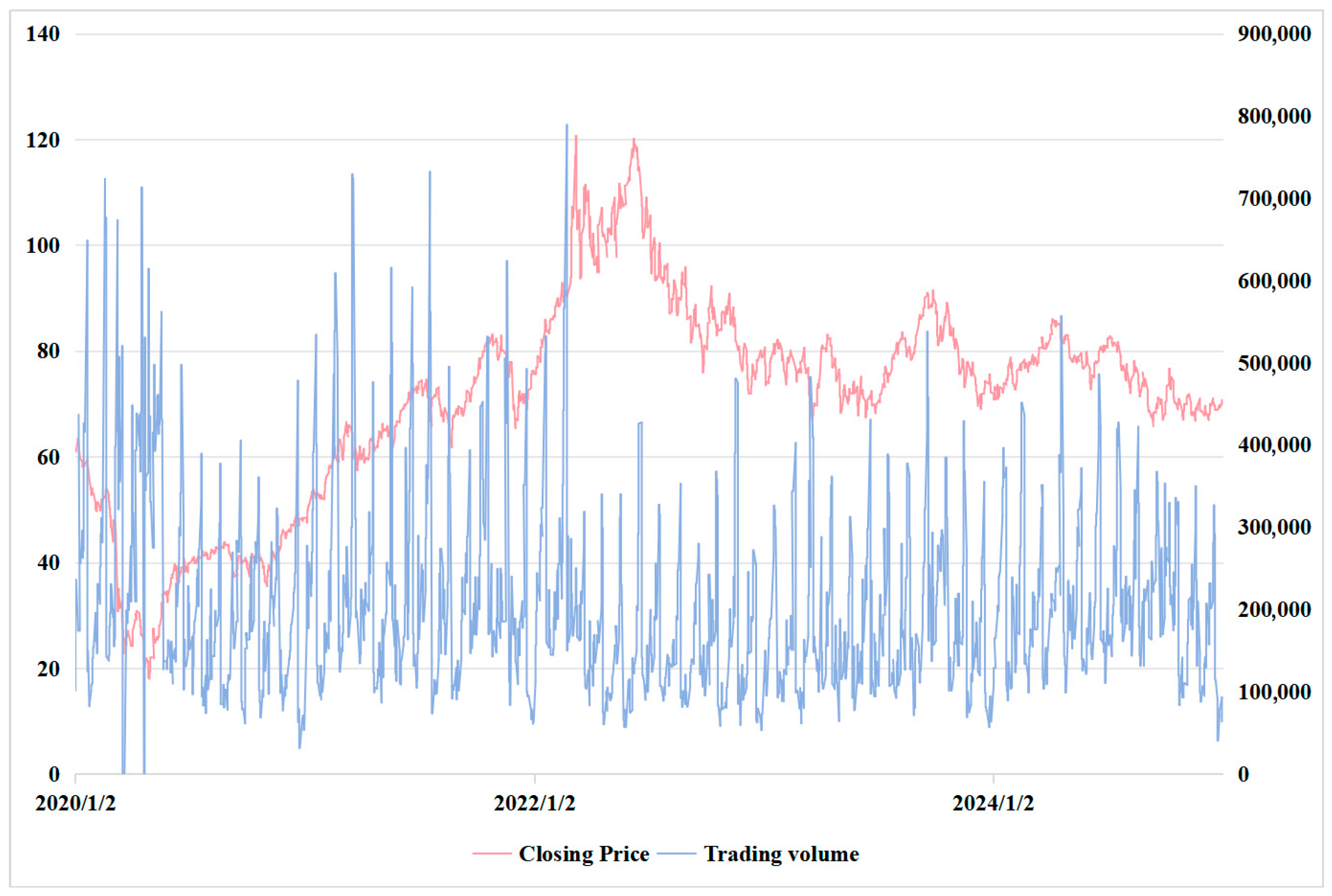
The sample period spans from 1 January 2020 to 31 December 2024 (Figure 2), based on the following considerations. First, this period captures significant economic events, including the sharp fluctuations in international oil prices caused by the COVID-19 pandemic, the subsequent price recovery during the post-pandemic economic rebound, and recent geopolitical disturbances affecting oil markets—making it highly representative in economic terms. Second, data completeness is ensured during this interval, which helps avoid estimation bias resulting from missing values or inconsistent frequency in historical datasets. Third, by using the most recent five full years of data, this study is able to reflect current market trends and provide a realistic basis for forecasting future developments. To systematically characterize the multidimensional drivers of crude oil futures prices, the external variables are categorized into three major groups, based on which the corresponding variable set is constructed. The detailed specification is presented in the subsequent section.

(1) Energy Futures Price Variables. Price fluctuations across different energy commodities often exhibit co-evolutionary characteristics, as crude oil is closely linked with other energy products in terms of production, consumption, storage, transportation, and financial attributes. To capture the interlinkages between crude oil and other energy markets, four representative indicators are selected as proxy variables in this study. Natural Gas Futures (NGN5): This reflects natural gas price trends in the United States and serves as a key indicator for industrial energy and heating markets. Fuel Oil Futures (NYFN5): Representing the prices of middle distillates, this variable is crucial for assessing the cost dynamics in the transportation and manufacturing sectors. Gasoline Futures (GPRN5): Based on the RBOB gasoline contract, it captures end-use energy consumption in the transportation sector. Carbon Emissions Futures (CFI2M5): Drawn from the EU Emissions Trading System (EU ETS), this variable reflects the carbon cost fluctuations under carbon pricing policies, thereby linking energy market pricing with environmental regulation.

(2) Macroeconomic Environment Variables. Crude oil futures prices are significantly influenced by the global macroeconomic climate. During periods of economic expansion, oil demand typically rises, while recessions tend to suppress price growth. To reflect macroeconomic conditions, four major stock indices are selected as proxy variables. S&P 500 Index (SPX): Comprising the 500 largest publicly traded companies in the U.S., it is one of the most widely used indicators of global economic performance. Dow Jones Industrial Average (DJI): Consisting of 30 leading industrial corporations, it serves as a barometer for traditional sector performance. NASDAQ Composite Index (IXIC): Focused on technology and innovation-driven firms, it provides insight into market risk sentiment. EURO STOXX 50 Index (STOXX50E): Composed of blue-chip stocks from leading eurozone economies, this index reflects the overall economic health of the euro area.

(3) Exchange Rates and Dollar-Related Variables. As crude oil is priced globally in U.S. dollars, fluctuations in the dollar exchange rate directly affect oil import costs for non-dollar economies and thus influence global demand. In addition, exchange rates indirectly impact oil prices via capital flows and portfolio adjustments. This study incorporates four exchange rate indicators. U.S. Dollar Index (DXY): A comprehensive measure of the dollar’s value relative to a basket of major currencies (including the euro, yen, pound sterling, Canadian dollar, Swedish krona, and Swiss franc), and one of the most commonly used gauges of dollar strength. USD/EUR and USD/JPY Exchange Rates: These represent the relative strength of the U.S. dollar against two of the world’s largest economies—the eurozone and Japan. CNY/USD Exchange Rate: This reflects the linkage between the Chinese economy and the global crude oil market, and also captures the impact of exchange rate volatility on the transaction costs of commodity trade.

All data are sourced from the Investing.com platform.

3.2. Methodology

This study develops a dynamic analytical framework based on the hypothesized interlinkages among the energy, financial, and foreign exchange markets to capture the multi-source driving characteristics of crude oil prices. Theoretically, oil prices are influenced not only by supply and demand fundamentals but also by financial market sentiment, risk premiums, and exchange rate fluctuations. Accordingly, the analytical approach employed in this paper—comprising the Augmented Dickey–Fuller (ADF) test, Granger causality test, cointegration analysis, and Johansen method—is designed to identify the dynamic dependence structures among the relevant variables from multiple dimensions and levels.

The construction of this framework is grounded in two theoretical rationales. First, drawing on the Efficient Market Hypothesis and Spillover Theory, this study utilizes correlation and causality analyses to trace the direction and lag structure of information transmission among key variables. Second, under the framework of Cointegration Theory, it further investigates whether a set of non-stationary variables exhibits an endogenous long-term equilibrium relationship, thus uncovering potential mechanisms of coordinated adjustment across markets.

3.2.1. Spearman Rank Correlation Method

While the correlation between variables can be visually observed through graphical methods such as scatter plots, a more rigorous approach involves calculating correlation coefficients. In this study, the Spearman rank correlation method is adopted because it does not require the assumption of normal distribution and is capable of capturing monotonic relationships between variables, whether linear or nonlinear. This makes it particularly suitable for analyzing economic and financial time series, which often exhibit nonlinearity and non-normality. The specific formula for the Spearman coefficient is presented in Equation (1).

$$\begin{array}{c}\rho =1-{\displaystyle \frac{6{\sum }_{i=1}^n{d}_i^2}{n\left(n^2-1\right)}}\end{array}$$

(1)

In the formula, $\rho$ represents the Spearman rank correlation coefficient, which ranges from −1 to 1. The term $d_i$ denotes the difference between the ranks of the $ith$ observation in the two variables. The variable $n$ refers to the total number of observations. When the ranks of the two variables are completely identical, $\rho =1$, indicating a perfect positive correlation. When the ranks are completely opposite, $\rho =-1$, indicating a perfect negative correlation. If there is no monotonic relationship between the variables, $\rho$ approaches 0.

3.2.2. Unit Root Inspection

The stationarity of time series was evaluated using the Augmented Dickey–Fuller (ADF) test [54]. The ADF test examines three regression specifications to accommodate different time series characteristics, as follows:

The model with trend and intercept is shown in Equation (2), which is suitable for series that show a deterministic trend.

$$\Delta y_t=c_0+c_{1}t+\gamma y_{t-1}+\sum _{j=1}^p{\varphi }_j\Delta y_{t-j}+{ϵ}_t$$

(2)

The model with intercept only is shown in Equation (3), which is suitable for series with non-zero mean but no trend.

$$\Delta y_t=c_0+\gamma y_{t-1}+\sum _{j=1}^p{\varphi }_j\Delta y_{t-j}+{ϵ}_t$$

(3)

The null hypothesis $H_0:\gamma =0$ (unit root present) is tested against $H_0:\gamma <0$ (stationary). If the ADF statistic falls below the critical value at the 5% significance level, $H_0$ is rejected, indicating stationarity $\left(I\right(0\left)\right)$. Non-stationary series are differenced until stationarity is achieved, with the integration order d determined as the minimum differencing required (denoted $I\left(d\right))$.

The optimal lag length $p$ was selected by minimizing the Akaike Information Criterion (AIC), as follows:

$$AIC=\mathit{ln}\left(2\pi \right)+\mathit{ln}{\sigma }^2+1+{\displaystyle \frac{2k}{n}}$$

(4)

where ${\sigma }^2$ is the residual variance, $k$ the number of estimated parameters, and $n$ the sample size.

3.2.3. Granger Causality Test

Sometimes, although a significant correlation exists between variables, such correlation does not necessarily imply a meaningful predictive relationship. Economic and financial time series often exhibit spurious correlations, where variables that are not substantively related may show high correlation coefficients due to shared trends or external shocks. These pseudo-correlations are misleading in the context of forecasting. Therefore, it is essential to examine dynamic causal relationships, for which the Granger causality test offers a widely accepted and theoretically grounded approach.

The Granger causality test is particularly suitable in this context, as it is designed to identify whether past values of one time series (X) contain information that helps predict another series (Y), beyond what is already explained by Y’s own history. This method involves two fundamental conditions: (1) changes in X must temporally precede changes in Y, and (2) the inclusion of lagged X values must significantly improve the predictive performance of the regression model for Y.

Compared with simple correlation analysis or contemporaneous regressions, Granger causality better captures the temporal structure of interactions between variables. It is especially useful for evaluating short-term predictive linkages in energy and financial markets, where volatility and interdependence are prominent. In this study, the Granger causality framework allows us to assess whether oil prices act as a leading indicator for downstream energy commodities, stock indices, and macroeconomic variables, or whether these variables in turn help forecast oil price fluctuations. By applying this method to first-differenced, stationary series, we ensure statistical rigor while extracting meaningful directional dependencies.

With reference to Ren et al. [55] and Raza and Alsulami [56], the standard test procedure for this paper includes the following steps:

Let $y_t$ and $x_t$ be two observed time series. First, estimate the unrestricted regression model, as follows:

$$y_t=c+\sum _{j=1}^m{\alpha }_j{y}_{\left\{t-j\right\}} +\sum _{i=1}^n{\beta }_i{x}_{\left\{t-i\right\}}+{\epsilon }_t$$

(5)

where $m$ and $n$ denote the optimal lag orders for $y_t$ and $x_t$, respectively, determined by criteria like AIC. The null hypothesis $H_0:{\beta }_1={\beta }_2=\cdots ={\beta }_{\mathrm{n}}=0$ asserts that $x_t$ does not Granger-cause $y_t$.

Let $S_0$ be the sum of squared residuals (SSR) from the restricted model (excluding $x_t$ terms), and $S_1$ the SSR from the unrestricted model. The F-test statistic is computed as follows:

$$F={\displaystyle \frac{ \left[\frac{S_{0 }-S_1}{n}\right]}{\left[\frac{S_1}{T-m-n-1}\right]}}$$

(6)

In Equation (6), $n$ denotes the number of lag terms of the explanatory variable $x_t$, which are excluded in the restricted model and tested for Granger causality. $m$ represents the number of lag terms of the dependent variable $y_t$, which are included in both the restricted and unrestricted models. The denominator degrees of freedom in the F-distribution, $T-m-n-1$, account for the number of observations $T$ minus the total number of parameters estimated in the unrestricted model, which includes $m$ lags of $y_t$, $n$ lags of $x_t$, and one intercept term.

To test for the reverse direction, i.e., whether $y_t$ Granger-causes $x_t$—the following unrestricted regression is estimated:

$$x_t=c+\sum _{j=1}^m{\gamma }_j{x}_{\left\{t-j\right\}}+\sum _{i=1}^n{\delta }_i{y}_{\left\{t-i\right\}}+{\nu }_t$$

(7)

The null hypothesis $H_0:{\beta }_1={\beta }_2=\cdots ={\beta }_{\mathrm{n}}=0$ implies that $y_t$ does not Granger-cause $x_t$. The F-statistic is constructed analogously to Equation (7), using the residual sum of squares from the restricted and unrestricted models.

To examine bidirectional causality, reverse the roles of $x_t$ and $y_t$ in the regression. If both directional tests reject their respective null hypotheses, we establish a feedback relationship between the variables.

3.2.4. Cointegration Analysis

Cointegration analysis aims to identify long-term equilibrium relationships among non-stationary time series. According to the seminal definition by Engle and Granger [57], if multiple variables are integrated of the same order) exhibit a linear combination ${\alpha }^{\prime }{y}_t$ (where $\mathsf{\alpha }={\left({\alpha }_1,{\alpha }_{2,}\dots ,{\alpha }_n\right)}^{\prime }$ is a cointegration vector) that reduces to a stationary series (i.e., ${\alpha }^{\prime }{y}_t\sim I\left(d-b\right)$), they are said to be cointegrated of order $\left(d,b\right)$, denoted as $y_t~CI\left(d,b\right)$.

For bivariate cases, the Engle–Granger two-step procedure verifies cointegration through the following workflow:

Confirm that both series share the same integration order. Estimate a regression model (Equation (8)) and test the stationarity of residuals (Equation (9)).

$$y_t=\alpha +\beta x_t+{ϵ}_t$$

(8)

$$\widehat{{ϵ}_t}=y_t-\widehat{\alpha }-\widehat{\beta }{x}_t$$

(9)

If the residuals are stationary ($I\left(0\right)$), cointegration is established, with ${(1, \widehat{\beta })}^{\prime }$ serving as the cointegration vector.

In multivariate systems, the Johansen cointegration test [58] transforms a $p$—order Vector Autoregressive (VAR) model (Equation (10)) into its error correction form (Equation (11)).

$$Y_t=A_1{Y}_{t-1}+\cdots +A_p{Y}_{t-p}+B{X}_t+{ϵ}_t$$

(10)

$$∆Y_t=\sum _{i=1}^{p-1}{\Gamma }_i∆Y_{i-i}+\prod Y_{t-1}+B{X}_t+{ϵ}_t$$

(11)

The cointegration rank $r$ (number of independent cointegration relationships) is determined via the trace statistic (Equation (12)).

$$Q_r=-T\sum _{i=r+1}^m\ln \left(1-{\lambda }_i\right)$$

(12)

where ${\lambda }_i$ are the eigenvalues of matrix $\Pi$ sorted in descending order, and $T$ is the sample size. The rejection of the null hypothesis $H_0$:at most $r$ cointegration relationships implies the system contains $m$ cointegration relationships.

4. Result

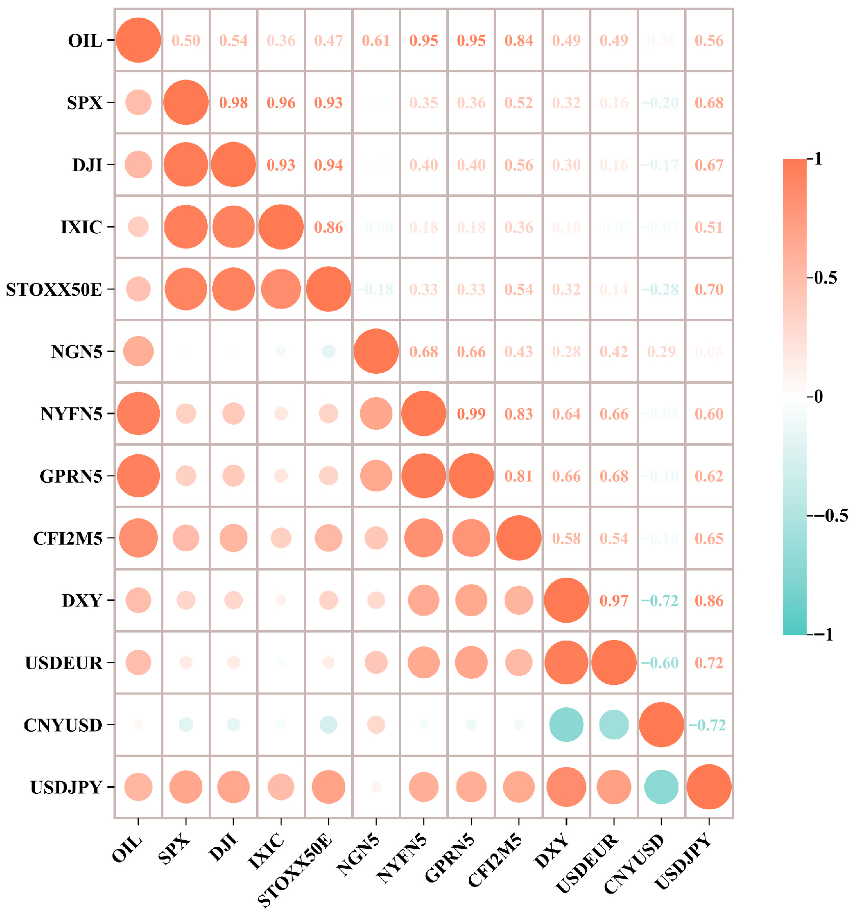
Figure 3 and

Table 1. Spearman correlation test results.

	OIL	SPX	DJI	IXIC	STOXX50E	NGN5	NYFN5	GPRN5	CFI2M5	DXY	USDEUR	CNYUSD	USDJPY
OIL	1
SPX	0.500 ***	1
DJI	0.539 ***	0.985 ***	1
IXIC	0.362 ***	0.963 ***	0.932 ***	1
STOXX50E	0.470 ***	0.929 ***	0.941 ***	0.865 ***	1
NGN5	0.615 ***	−0.015	0.01	−0.084 ***	−0.183 ***	1
NYFN5	0.949 ***	0.353 ***	0.402 ***	0.178 ***	0.329 ***	0.675 ***	1
GPRN5	0.946 ***	0.360 ***	0.400 ***	0.183 ***	0.328 ***	0.657 ***	0.994 ***	1
CFI2M5	0.838 ***	0.520 ***	0.558 ***	0.360 ***	0.541 ***	0.429 ***	0.832 ***	0.809 ***	1
DXY	0.493 ***	0.315 ***	0.305 ***	0.103 ***	0.318 ***	0.284 ***	0.640 ***	0.660 ***	0.577 ***	1
USDEUR	0.491 ***	0.161 ***	0.157 ***	−0.053 *	0.143 ***	0.422 ***	0.658 ***	0.678 ***	0.535 ***	0.968 ***	1
CNYUSD	0.062 **	−0.202 ***	−0.166 ***	−0.069 **	−0.282 ***	0.294 ***	−0.077 ***	−0.102 ***	−0.097 ***	−0.725 ***	−0.603 ***	1
USDJPY	0.561 ***	0.682 ***	0.670 ***	0.514 ***	0.698 ***	0.084 ***	0.605 ***	0.621 ***	0.649 ***	0.863 ***	0.724 ***	−0.716 ***	1

Note: *** means rejecting the null hypothesis of no causal relationship between sequences at the significance level of 1%, ** means rejecting the null hypothesis of no causal relationship between sequences at the significance level of 5%, * means rejecting the null hypothesis of no causal relationship between sequences at the significance level of 10%.

present the correlation results based on the Spearman method using the original data. The results indicate that OIL exhibits statistically significant nonparametric correlations with most macro-financial variables, with the strength and direction of the relationships varying by variable category. Regarding stock indices, OIL is positively and significantly correlated with the DJI, SPX, and STOXX50E, with Spearman correlation coefficients of 0.539, 0.500, and 0.470, respectively. This suggests a strong comovement between crude oil prices and major global equity markets, highlighting the systemic role of oil as a risk asset in portfolio allocation. In the energy market, OIL shows strong positive correlations with NYFN5 and GPRN5, both exceeding 0.94, and also with NGN5 (0.615), indicating close linkages in supply-demand structures and price co-movements between crude oil and downstream energy products. Additionally, the correlation coefficient between OIL and CFI2M5 is 0.838, suggesting that carbon prices may serve as a complementary indicator for oil price fluctuations. Among the exchange rate variables, OIL is positively correlated with the U.S. Dollar Index (DXY, 0.493) and with the USD/EUR exchange rate (0.491). In contrast, its correlation with the CNY/USD exchange rate is relatively weak (0.062), and only marginally significant at the 10% level, indicating a lower degree of linkage with emerging market currencies. Overall, these results demonstrate that OIL exhibits substantial cross-asset correlations, particularly with other energy commodities and dollar-denominated financial instruments.

Figure 4 and

Table 2. Results of the correlation test with one period lag for relevant variables.

	OIL	LSPX	LDJI	LIXIC	LSTOXX50E	LNGN5	LNYFN5	LGPRN5	LCFI2M5	LDXY	LUSDEUR	LCNYUSD	LUSDJPY
OIL	1
LSPX	0.506 ***	1
LDJI	0.545 ***	0.985 ***	1
LIXIC	0.369 ***	0.963 ***	0.932 ***	1
LSTOXX50E	0.472 ***	0.930 ***	0.942 ***	0.865 ***	1
LNGN5	0.617 ***	−0.016	0.008	−0.086 ***	−0.185 ***	1
LNYFN5	0.945 ***	0.356 ***	0.404 ***	0.180 ***	0.329 ***	0.675 ***	1
LGPRN5	0.941 ***	0.361 ***	0.400 ***	0.184 ***	0.327 ***	0.657 ***	0.993 ***	1
LCFI2M5	0.838 ***	0.521 ***	0.559 ***	0.360 ***	0.541 ***	0.430 ***	0.833 ***	0.808 ***	1
LDXY	0.491 ***	0.307 ***	0.297 ***	0.092 ***	0.312 ***	0.287 ***	0.643 ***	0.662 ***	0.577 ***	1
LUSDEUR	0.489 ***	0.152 ***	0.149 ***	−0.064 **	0.137 ***	0.425 ***	0.660 ***	0.679 ***	0.535 ***	0.968 ***	1
LCNYUSD	0.067 **	−0.193 ***	−0.158 ***	−0.059 *	−0.276 ***	0.295 ***	−0.076 **	−0.100 ***	−0.094 ***	−0.722 ***	−0.600 ***	1
LUSDJPY	0.561 ***	0.677 ***	0.665 ***	0.506 ***	0.694 ***	0.087 ***	0.610 ***	0.623 ***	0.650 ***	0.862 ***	0.723 ***	−0.714 ***	1

Note: LSPX refers to the first-order lag of SPX, and so on; *** means rejecting the null hypothesis of no causal relationship between sequences at the significance level of 1%, ** means rejecting the null hypothesis of no causal relationship between sequences at the significance level of 5%, * means rejecting the null hypothesis of no causal relationship between sequences at the significance level of 10%.

present the Spearman correlation results based on the one-period lagged variables. After incorporating one-period lagged variables, the Spearman correlation test results largely preserve the original correlation structure among variables, indicating that the crude oil market continues to exhibit a significant short-term lagged response to macro-financial factors. The correlations between OIL and energy-related variables—namely LNYFN5, LGPRN5, and LCFI2M5—remain particularly strong, with coefficients of 0.945, 0.941, and 0.838, respectively. This suggests a high degree of inertia in the price co-movements across energy commodities. The correlations between OIL and major stock indices such as LSPX, LDJI, and LIXIC remain moderate (approximately 0.5), indicating a stable dynamic coupling between crude oil prices and financial market fluctuations. In terms of exchange rates, OIL maintains positive correlations with LDXY and LUSDEUR (both around 0.49), suggesting that the dollar-based pricing mechanism continues to influence oil prices even with a temporal lag. The negative correlation with LCNYUSD slightly strengthens (−0.067), though it remains relatively weak, implying limited spillover from emerging market currencies. Notably, the correlation between OIL and LUSDJPY reaches 0.561, highlighting a potential indirect transmission channel from USD/JPY movements to oil prices, possibly through shifts in global risk appetite or currency arbitrage mechanisms.

4.1. Unit Root Inspection Results

To examine the stationarity of the OIL series, the Augmented Dickey–Fuller (ADF) unit root test is employed, with the results presented in

Table 3. Unit root test results of different lags.

Test Type	Lag	ADF Statistic	Critical Value (1%)	Critical Value (5%)	Critical Value (10%)	p-Value	Significance
Level	0	−3.446	−3.430	−2.860	−2.570	0.0095	***
Level	1	−2.786	−3.430	−2.860	−2.570	0.0603	*
Level	2	−1.843	−3.440	−2.872	−2.57-	0.3595
Level	3	−1.561	−3.470	−2.883	−2.573	0.5029

Note: *** means rejecting the null hypothesis of non-stationarity of the series at the significance level of 1%, * means rejecting the null hypothesis of no causal relationship between sequences at the significance level of 10%.

. The results indicate that the OIL series exhibits a certain degree of stationarity in its level form. When the lag order is set to zero, the ADF test statistic is −3.446, which is significantly lower than the 1% and 5% critical values (−3.430 and −2.860, respectively), with a corresponding p-value of 0.0095. This allows for the rejection of the null hypothesis, suggesting that the OIL series is stationary at this lag level. However, as the lag order increases, the statistical significance of the test results gradually weakens. At a lag of one, the ADF statistic is −2.786, which is close to the 5% critical value, but with a p-value of 0.0603, the null hypothesis can only be rejected at the 10% significance level. When the lag is increased to two and three, the ADF statistics decline to −1.843 and −1.561, respectively, failing to meet any conventional significance thresholds and thus providing insufficient evidence to reject the null hypothesis. These results suggest that while the OIL series demonstrates weak stationarity at lower lag orders, the presence of a unit root cannot be ruled out for the full sample. Consequently, the subsequent analysis will examine the stationarity of the differenced series to ensure the robustness and validity of the modeling process.

Apart from OIL, the stationarity of the remaining twelve variables requires further examination. The test results are presented in

Table 4. ADF test results for all variables.

Variable	Lag	ADF Statistic	Critical Value (1%)	Critical Value (5%)	Critical Value (10%)	p-Value	Significance
OIL	0	−3.446	−3.430	−2.860	−2.570	0.0094	***
SPX	3	−1.101	−3.474	−2.883	−2.573	0.715
DJI	0	−1.278	−3.430	−2.860	−2.570	0.639
IXIC	3	−1.733	−3.474	−2.883	−2.573	0.414
STOXX50E	0	−0.835	−3.430	−2.860	−2.570	0.809
NGN5	0	−0.979	−3.430	−2.860	−2.570	0.761
NYFN5	0	−1.491	−3.430	−2.860	−2.570	0.538
GPRN5	0	−2.604	−3.430	−2.860	−2.570	0.092	*
CFI2M5	0	−1.718	−3.430	−2.860	−2.570	0.422
DXY	3	−0.850	−3.474	−2.883	−2.573	0.804
USDEUR	0	−0.938	−3.430	−2.860	−2.570	0.775
CNYUSD	3	−1.512	−3.474	−2.883	−2.573	0.528
USDJPY	3	−1.876	−3.474	−2.883	−2.573	0.344

Note: *** means rejecting the null hypothesis of non-stationarity of the series at the significance level of 1%, * means rejecting the null hypothesis of no causal relationship between sequences at the significance level of 10%.

. Following unit root tests on OIL and the remaining financial variables, the results reveal that OIL is stationary at the level when no lag is included. Specifically, the ADF test statistic for OIL is −3.446, which is significantly lower than the 1% critical value (−3.430), with a corresponding p-value of 0.0094. This strongly rejects the null hypothesis of a unit root, indicating that the OIL series achieves stationarity at the level with no lag. In contrast, most of the other variables fail to pass the unit root test, demonstrating clear non-stationary behavior. For instance, at a lag order of zero, the ADF statistics for STOXX50E, NYFN5, NGN5, and CFI2M5 are −0.835, −1.491, −0.979, and −1.718, respectively, all with p-values well above 0.1. These results do not allow for the rejection of the null hypothesis, indicating the presence of unit roots. Notably, the ADF statistic for GPRN5 is −2.604, which is close to the 10% critical value (−2.570), with a p-value of 0.092. This suggests a tendency toward weak stationarity. Regarding exchange rate variables, USDEUR and CNYUSD report ADF statistics of −0.938 and −1.512, with corresponding p-values of 0.775 and 0.528, respectively—both failing to meet standard significance thresholds for stationarity. Additionally, when lagged three periods, DXY and USDJPY yield ADF statistics of −0.850 and −1.876, with p-values of 0.804 and 0.344, respectively. These results also support the conclusion that the series exhibits strong unit root characteristics.

Table 5. ADF test results for the first-order differences of relevant sequences.

Variable	Lag Order	ADF Statistic	p-Value
OIL	2	−12.074	0.000 ***
SPX	2	−8.305	0.000 ***
DJI	2	−8.760	0.000 ***
IXIC	2	−8.984	0.000 ***
STOXX50E	2	−6.190	0.000 ***
NGN5	2	−11.102	0.000 ***
NYFN5	2	−9.693	0.000 ***
GPRN5	2	−11.607	0.000 ***
CFI2M5	2	−9.552	0.000 ***
DXY	2	−5.020	0.000 ***
USDEUR	2	−5.00	0.000 ***
CNYUSD	2	−7.920	0.000 ***
USDJPY	2	−5.340	0.000 ***

Note: *** means rejecting the null hypothesis of non-stationarity of the series at the significance level of 1%.

presents the ADF test results for all variables after first-order differencing. Compared with the widespread non-stationarity observed in the original series, all variables exhibit significant stationarity after differencing. Specifically, the ADF test statistic for the first difference of OIL is −12.074, while those for SPX, DJI, and IXIC are −8.305, −8.760, and −8.984, respectively—all substantially below the 1% critical value threshold and associated with p-values of 0.000, indicating strong statistical significance. A similar pattern is observed among the energy-related variables; the ADF statistics for NGN5, NYFN5, GPRN5, and CFI2M5 are −11.102, −9.693, −11.607, and −9.552, respectively, all suggesting that these series become stationary after first differencing. For exchange rates and other macroeconomic indicators, the first-differenced ADF statistics for DXY, USDEUR, CNYUSD, and USDJPY are −5.020, −5.000, −7.920, and −5.340, respectively. These values are also significantly below their corresponding critical thresholds, further confirming the statistical stationarity of these series at the first-difference level. Overall, the results validate that all variables in the dataset are integrated of order one, i.e., I(1) processes. This finding provides the necessary prerequisite for subsequent cointegration testing and model development.

4.2. Granger Test Results

To ensure the validity of the Granger causality analysis, all variables were first tested for stationarity using the ADF unit root test. The results confirm that most variables are I(1) processes. Therefore, Granger causality tests were conducted on the first-differenced series to satisfy the stationarity requirement.

As can be seen from

Table 6. Granger test results of OIL and relevant economic variables.

Variable Pair		F-Statistic	p-Value
D_OIL	D_SPX	0.439	0.645
D_OIL	D_DJI	0.541	0.582
D_OIL	D_IXIC	0.139	0.870
D_OIL	D_STOXX50E	2.440	0.088
D_OIL	D_NGN5	3.055	0.048 *
D_OIL	D_NYFN5	7.879	0.000 **
D_OIL	D_GPRN5	7.393	0.001 **
D_OIL	D_CFI2M5	0.474	0.622
D_OIL	D_DXY	0.076	0.927
D_OIL	D_USDEUR	0.312	0.732
D_OIL	D_CNYUSD	2.972	0.052
D_OIL	D_USDJPY	1.292	0.275
D_SPX	D_OIL	5.266	0.005 **
D_DJI	D_OIL	2.741	0.065
D_IXIC	D_OIL	6.127	0.002 **
D_STOXX50E	D_OIL	1.874	0.154
D_NGN5	D_OIL	3.395	0.034 *
D_NYFN5	D_OIL	5.089	0.006 **
D_GPRN5	D_OIL	6.731	0.001 **
D_CFI2M5	D_OIL	2.759	0.064
D_DXY	D_OIL	0.606	0.546
D_USDEUR	D_OIL	1.137	0.321
D_CNYUSD	D_OIL	0.494	0.611
D_USDJPY	D_OIL	1.530	0.217

Note: ** means rejecting the null hypothesis of no causal relationship between sequences at the significance level of 5%; * means rejecting the null hypothesis of no causal relationship between sequences at the significance level of 10%.

, when OIL is specified as the dependent variable, NGN5 (p = 0.048), NYFN5 (p = 0.000), and GPRN5 (p = 0.001) exhibit statistically significant Granger causality, indicating that fluctuations in natural gas, fuel oil, and gasoline futures prices can effectively predict changes in crude oil prices. This finding reveals a strong interconnectedness between crude oil and downstream energy commodities and reflects the stage-wise transmission of price signals along the energy value chain. Conversely, when OIL is treated as an explanatory variable, it also Granger-causes NYFN5 (p = 0.006) and GPRN5 (p = 0.001), further underscoring crude oil’s role as a pricing anchor in global energy markets and its influence on downstream market expectations and trading behaviors.

Moreover, OIL demonstrates significant Granger causality toward SPX (p = 0.005) and IXIC (p = 0.002), suggesting that oil prices not only serve as key indicators within the energy sector but also exert broader influence on financial markets. Through channels such as corporate cost structures, inflation expectations, and investor risk sentiment, crude oil price dynamics can partially steer stock market movements. This linkage is particularly salient amid the current backdrop of global energy transitions and geopolitical tensions, where oil price shocks increasingly resonate across asset classes.

Notably, no significant Granger causality is observed between OIL and any of the exchange rate variables (DXY, USDEUR, CNYUSD, USDJPY), with bidirectional p-values exceeding conventional significance thresholds. While this may initially appear counterintuitive, it can be theoretically justified. On one hand, although crude oil is denominated in U.S. dollars, exchange rate movements primarily reflect a complex interplay of macroeconomic fundamentals and monetary policy expectations, which may respond to oil price fluctuations with a lag or be shaped by broader systemic risks. On the other hand, as a globally traded commodity, crude oil prices are highly market-oriented and often dominated by factors such as supply-demand expectations, geopolitical developments, and speculative behavior in futures markets, thereby diluting the direct impact of any single currency’s exchange rate.

4.3. Cointegration Test Results

Cointegration analysis is an important method to test whether there is a long-term equilibrium relationship between sequences. This paper uses the Engle–Granger two-step method to test the cointegration of crude oil futures prices and relevant economic time series. The results of the cointegration test between sequences are summarized in

Table 7. Co-integration test results of the EG method.

	Cointegration Coefficient	ADF Statistic	p-Value
OIL & SPX	0.013	−3.751	0.019
OIL & DJI	0.002	−3.861	0.014
OIL & IXIC	0.003	−3.712	0.022
OIL & STOXX50E	0.016	−3.862	0.014
OIL & NGN5	6.421	−4.670	0.000
OIL & NYFN5	23.436	−4.026	0.008
OIL & GPRN5	0.074	−4.959	0.000
OIL & CFI2M5	0.703	−4.413	0.002
OIL & DXY	1.637	−3.061	0.116
OIL & USDEUR	198.159	−3.220	0.081
OIL & CNYUSD	170.609	−3.785	0.017
OIL & USDJPY	0.583	−3.474	0.042

.

The results indicate that OIL and major stock indices—including SPX (p = 0.019), DJI (p = 0.014), IXIC (p = 0.022), and STOXX50E (p = 0.014)—all pass the unit root test at the 5% significance level, confirming the existence of significant cointegration relationships between crude oil prices and key capital market indicators. This finding further supports the results of the Granger causality analysis, suggesting that oil prices not only have short-term predictive power over financial markets but are also structurally linked to equity markets in the long run. It underscores the deep coupling between energy prices and broader macroeconomic fundamentals.

In the energy sector, OIL shows strong and stable long-term cointegration relationships with NGN5 (p = 0.000), NYFN5 (p = 0.008), GPRN5 (p = 0.000), and CFI2M5 (p = 0.002), with notably large coefficients. In particular, the coefficients for NYFN5 (23.436) and NGN5 (6.421) are highly significant, indicating a strong co-movement between crude oil and downstream energy products such as natural gas and fuel oil. These results are economically plausible and can be interpreted through the lenses of supply-demand structures, substitution effects, and interdependencies along the energy value chain.

For exchange rate variables, while some bivariate relationships—such as OIL with CNYUSD (p = 0.017) and USDJPY (p = 0.042)—exhibit significant cointegration, their overall stability is notably weaker than that of stock indices and energy prices. For instance, OIL’s relationships with DXY (p = 0.116) and USDEUR (p = 0.081) approach the 10% significance threshold but remain statistically insignificant. This is understandable given that exchange rate dynamics are shaped by a complex array of international financial factors, of which oil prices are only one component. Thus, although crude oil does not exert a significant short-term causal effect on exchange rates, its long-run equilibrium relationships with certain currencies suggest structural or expectation-driven linkages rather than direct, high-frequency transmission effects.

In addition, this study employs the Johansen method to examine the time series of crude oil futures prices and selected economic variables. Given the large number of relevant variables previously identified and the high degree of correlation among many of them, only a subset of variables is included in this test. Based on the criteria that only one variable from each group of similar explanatory variables is highly correlated with OIL or passes the Granger causality test, SPX, GPRN5, and USDEUR are ultimately selected. The cointegration test results are presented in

Table 8. Johansen Cointegration Test Results.

Null Hypothesis	Eigenvalue	Trace Statistic	Critical Values	Conclusion (5% Level)
No cointegration (r = 0)	0.26	790.336 ***	37.034 (10%)	Rejected (Strong cointegration)
			40.175 (5%)
			46.572 (1%)
At most 1 coint. (r ≤ 1)	0.248	391.147 ***	21.778 (10%)	Rejected (≥2 coint. vectors)
			24.276 (5%)
			29.515 (1%)
At most 2 coint. (r ≤ 2)	0.009	12.492 *	10.474 (10%)	Rejected at 10% (≥3 coint. vectors)
			12.321 (5%)
			16.364 (1%)
At most 3 coint. (r ≤ 3)	0	0.115	2.976 (10%)	Not rejected (Final rank: r = 3)
			4.130 (5%)
			6.941 (1%)

Note: *** means rejecting the null hypothesis of no causal relationship between sequences at the significance level of 1%, * means rejecting the null hypothesis of no causal relationship between sequences at the significance level of 10%.

.

The results show that under the null hypothesis of “no cointegration (r = 0),” the trace statistic is 790.336, which greatly exceeds the critical values at the 1 percent, 5 percent, and 10 percent levels. This leads to a significant rejection of the null hypothesis, indicating the presence of at least one cointegrating vector among the four variables, and thus a stable long-term equilibrium relationship. As the number of cointegrating vectors increases, the test continues to reject the null hypothesis of “at most one cointegration relationship (r ≤ 1),” with a corresponding trace statistic of 391.147, again well above the critical values. This suggests the existence of at least two cointegrating vectors, providing further statistical evidence of long-term interdependence among the variables.

When assuming “at most two cointegrating relationships (r ≤ 2),” the trace statistic is 12.492, slightly exceeding the 10 percent critical value of 10.474 and approaching the 5 percent critical value of 12.321. This indicates that the test marginally passes at the 10 percent significance level, suggesting the possible existence of a third cointegrating relationship within the system. Finally, under the assumption of “at most three cointegrating relationships (r ≤ 3),” the trace statistic is 0.115, which is significantly lower than all critical values, leading to a failure to reject the null hypothesis. This confirms that the cointegration rank is three.

Therefore, there exist three statistically significant cointegrating vectors among OIL, SPX, GPRN5, and USDEUR at the system level. This implies not only the presence of a stable long-term equilibrium relationship among these variables but also a multivariate structural feature that warrants deeper interpretation. Specifically, the inclusion of SPX suggests that oil price dynamics are intrinsically linked to equity market performance, potentially reflecting broader macroeconomic expectations and investor sentiment. Meanwhile, the cointegration between OIL and GPRN5 underscores the structural interdependence within the energy value chain, particularly the pricing transmission mechanisms between upstream crude oil and downstream refined products like gasoline. The involvement of USDEUR further highlights the role of currency markets in mediating global commodity pricing, suggesting that exchange rate movements may influence oil price equilibrium through trade, valuation, and liquidity channels.

4.4. Error Correction Model Estimation

Given that all-time series under investigation are integrated of order one [I(1)] and most exhibit statistically significant cointegration relationships with crude oil prices—confirmed by both the Engle–Granger and Johansen tests—the Error Correction Model (ECM) is employed to capture both the short-term dynamics and long-run equilibrium adjustments of the oil price system.

The estimation results are presented in

Table 9. Estimation Results of the Error Correction Model.

VARIABLES	ECM_Model
L.d_SPX	0.00443
	(0.00428)
L.d_IXIC	−0.000197
	(0.000868)
L.d_STOXX50E	0.00157
	(0.00191)
L.d_NGN5	1.146 ***
	(0.359)
L.d_NYFN5	3.466
	(2.138)
L.d_GPRN5	−0.00456
	(0.00536)
L.d_CFI2M5	−0.0797 **
	(0.0371)
L.d_DXY	0.0319
	(0.554)
L.d_USDEUR	46.17
	(48.45)
L.d_CNYUSD	348.0 *
	(190.3)
L.d_USDJPY	−0.191 *
	(0.115)
L.ecm_term	−0.0910 ***
	(0.0223)
Constant	−0.00259
	(0.0658)
Observations	715
R-squared	0.060

Note: *** means rejecting the null hypothesis of no causal relationship between sequences at the significance level of 1%; ** means rejecting the null hypothesis of no causal relationship between sequences at the significance level of 5%; * means rejecting the null hypothesis of no causal relationship between sequences at the significance level of 10%, Standard errors in parentheses.

. Among the short-run variables, L.d_NGN5 and L.d_CFI2M5 exhibit statistically significant effects on crude oil price changes at the 1% and 5% significance levels, respectively. Additionally, the L.d_CNYUSD and L.d_USDJPY also show marginal significance (p < 0.1), suggesting exchange rate fluctuations play a partial role in short-run oil price volatility. The error correction term (L.ecm_term) is significantly negative (−0.0910, p < 0.01), indicating that the crude oil market exhibits a stable adjustment mechanism toward its long-run equilibrium; approximately 9.1% of the disequilibrium from the previous period is corrected in each time step.

Despite the fact that several variables (e.g., stock indices and exchange rates) are not statistically significant in the short run, they are retained in the final model. This inclusion is supported by their cointegrating relationships with oil prices, as well as their theoretical and structural relevance in shaping expectations and market interactions. Such a specification enables the model to maintain both econometric completeness and interpretative consistency across time horizons.

The final ECM used to explain crude oil price dynamics can be expressed as follows:

$$\Delta OI{L}_t=\mathsf{\alpha }+\sum _{i=1}^k{\beta }_i\Delta X_{i,t-1}+\lambda \cdot EC{M}_{t-1}+{\epsilon }_t$$

where $\Delta OI{L}_t$ denotes the first difference of crude oil prices, $\Delta X_{i,t-1}$ represents the first differences of the macro-financial variables lagged by one period, $EC{M}_{t-1}$ is the error correction term constructed from cointegration residuals, reflecting the magnitude of deviation from the long-run equilibrium state, and $\lambda <0$ constitutes the adjustment coefficient. After incorporating the estimation results, the specific model takes the following form:

$$\begin{gathered} \Delta OI{L}_t=-0.00259+0.00443\cdot \Delta SP{X}_{t-1}-0.000197\cdot \Delta IXI{C}_{t-1}+0.00157\cdot \Delta STOXX50E_{t-1} \\ +{1.146}^{***}\Delta NGN{5}_{t-1}+3.466\cdot \Delta NYFN{5}_{t-1}-0.00456\cdot \Delta GPRN{5}_{t-1} \\ -{0.0797}^{**}\Delta CFI2M{5}_{t-1}+0.0319\cdot \Delta DX{Y}_{t-1}+46.17\cdot \Delta USDEU{R}_{t-1} \\ +{348.0}^{*}\Delta CNYUS{D}_{t-1}-{0.191}^{*}\cdot \Delta USDJP{Y}_{t-1}-{ 0.0910}^{***}\cdot EC{M}_{t-1}+{\epsilon }_t \end{gathered}$$

Overall, the final model not only depicts the short-term volatility path of crude oil prices (especially the immediate impact of energy futures and some exchange rate indicators), but also reflects the mechanism of adjustment toward a long-term equilibrium state. This “short-term-long-term” combined modeling approach enhances the explanatory power and predictive power of oil price dynamics in a highly volatile market environment.

5. Discussion

This study corroborates the findings of existing literature regarding the significant influence of macroeconomic fundamentals [59,60] and energy prices [3,8] on crude oil futures prices. However, it reveals discrepancies concerning the importance of exchange rate factors compared to some prior studies [61,62]. Empirical results indicate that although exchange rate variables exhibit long-term cointegration relationships with crude oil futures prices, their explanatory power in the short term remains relatively weak. This may be attributed to the high-frequency data employed herein and the increasingly decoupled dynamic structure between financial and energy markets.

Building on this, the present study further emphasizes the strategic significance of crude oil futures price forecasting amid the global energy transition. Diverging from traditional views that regard oil prices merely as financial assets [63], this research posits that their more critical role lies in providing forward-looking signals. Enhancing price forecast accuracy can aid policymakers and investors in proactively identifying risks associated with market volatility [5,64], thereby mitigating the likelihood of stranded assets, capital misallocation, and delays in infrastructure adjustments. This contributes to creating a more controllable external environment conducive to a low-carbon transition.

Although the proposed model demonstrates robust short-term forecasting performance, its applicability to medium- and long-term predictions warrants further validation. Moreover, despite employing a series of empirical tools to uncover the multifaceted linkages among crude oil prices, financial markets, exchange rates, and energy markets, this study—limited by scope and timeliness—has yet to integrate these findings into a unified dynamic forecasting framework. Future research could extend this work by developing linear or nonlinear vector error correction models (VECM), structural VAR models, or nonlinear causal network models to further investigate impulse response paths, asymmetric behaviors, and structural stability within multivariate systems, thereby enhancing the explanatory power and predictive accuracy of oil price dynamics.

6. Conclusions and Policy Implications

6.1. Conclusions and Limitations

Based on a review of the theoretical foundations of oil futures price composition, this paper identifies the core factors influencing oil futures price fluctuations. Under the current trading structure, which is predominantly based on cash-settled contracts, oil futures prices primarily reflect market participants’ expectations of future spot prices, rather than a direct aggregation of crude oil production costs, taxes, and distribution expenses. The anticipatory nature of the futures market and strategic interactions among traders play a dominant role in price formation. Recognizing this, the paper argues that improving the precision of oil futures forecasting is essential for enabling adaptive transition pathways—particularly under rising uncertainty and volatility in global energy markets. A more accurate representation of price expectations informs infrastructure investment cycles, reduces carbon lock-in risks, and assists in synchronizing fossil phase-out strategies with renewable scale-up plans. Drawing on an in-depth analysis of the oil futures market, this paper establishes an econometric approach, with the main conclusions summarized as follows:

(1) Empirical results indicate that oil futures prices are significantly correlated with other energy prices, macroeconomic variables, and exchange rate factors. Among these, the level of economic development serves as a key driver of oil futures price changes, while the impact of exchange rate factors appears to be insignificant based on the daily data utilized in this study.

(2) Further cointegration tests reveal the existence of long-term equilibrium relationships between oil futures prices and variables such as macroeconomic conditions, exchange rate levels, and energy prices, underscoring the complexity and multifactor-driven nature of the price formation mechanism.

(3) The ECM estimation results indicate that certain energy prices (e.g., natural gas and fuel oil) exert statistically significant short-run effects on crude oil futures, while the error correction term is both negative and highly significant, confirming the existence of a stable long-run relationship and a moderate speed of adjustment toward equilibrium.

(4) The forecasting method proposed in this paper accounts for the nonlinear and highly volatile characteristics of oil futures prices. It demonstrates good performance in short-term forecasting, enhancing the model’s ability to adapt to market noise and structural changes.

6.2. Policy Implications

Based on the findings of this study, the following policy recommendations are proposed to enhance the functional role of the oil futures market and stabilize price expectations:

(1) Strengthen market monitoring and information disclosure mechanisms. Governments should enhance real-time supervision of the futures market, improve price early warning systems, increase information transparency, and curb excessive speculation, thereby ensuring that futures prices reasonably reflect market fundamentals and macroeconomic expectations.

(2) Improve the system of energy price risk management tools. Enterprises—particularly those in high-carbon industries—should be encouraged to make rational use of financial instruments such as futures to manage the risks associated with energy price volatility. This would enhance the stability of green investment decisions and provide a risk buffer for advancing the transition to sustainable development.

(3) Promote the integrated development of green finance and the futures market. Efforts should be made to incorporate indicators such as carbon prices and green investment metrics into energy futures analysis models, thereby constructing a price discovery and risk pricing mechanism that serves the needs of a low-carbon economy and guides resource allocation toward the green energy sector.