Transient Stability Assessment of Power Systems Built upon Attention-Based Spatial–Temporal Graph Convolutional Networks

Abstract

Rapid and accurate transient stability assessment (TSA) is crucial for ensuring secure and stable operation in power systems. However, existing methods fail to adequately exploit the spatiotemporal characteristics in power grid transient data, which constrains the evaluation performance of models. This paper proposes a TSA method built upon an Attention-Based Spatial–Temporal Graph Convolutional Network (ASTGCN) model. First, a spatiotemporal attention module is used to aggregate and extract the spatiotemporal correlations of the transient process in the power system. A spatiotemporal convolution module is then employed to effectively capture the spatial features and temporal evolution patterns of transient stability data. In addition, an adaptive focal loss function is designed to enhance the fitting of unstable samples and increase the weight of misclassified samples, thereby improving global accuracy and reducing the occurrence of missed instability samples. Finally, the simulation results from the New England 10-machine 39-bus system and the NPCC 48-machine 140-bus system validate the effectiveness of the proposed methodology.

1. Introduction

The rapid and accurate perception of power system operational status, serving as a proactive safeguard, ensures the secure and stable operation of the grid. As the integration of power electronic devices and the penetration of renewable energy increase in the grid, the new power system, dominated by renewable energy, exhibits complex and dynamic structural and operational characteristics. As a result, the transient stability risks faced by the grid are becoming increasingly severe, leading to occasional collapses of the power system [1]. Therefore, it has become urgent to timely identify potential transient rotor angle stability risks to ensure the safe and stable operation of the grid under the new circumstances.

Traditional transient stability assessment (TSA) methods for power systems can be categorized into time-domain simulation methods [2] and direct methods [3]. Both approaches rely on stability mechanism-based analytical techniques to determine transient stability, and they are dependent on the accuracy of system modeling and computational resources. This makes it difficult to meet the demands of modern power system security assessment.

In recent years, with the deployment of wide-area measurement systems and digital intelligence technologies, data-driven approaches based on machine learning have provided new insights for the rapid and accurate perception of the complex and dynamic operational status of power systems [4]. In the early stages of machine learning development, scholars extensively explored the application of shallow machine learning methods, including Decision Tree (DT) [5], Support Vector Machine (SVM) [6], Random Forest (RF) [7], and k-Nearest Neighbors (KNN) [8], in TSA. The limited data mining capabilities of shallow machine learning methods impose constraints on their generalization ability, particularly when handling complex transient stability data [9]. With the rapid development of deep learning and its superior performance in feature extraction, several representative deep learning algorithms, including Convolutional Neural Networks (CNNs) [10], Deep Belief Networks (DBNs) [11], Stacked Autoencoders (SAEs) [12], and Long Short-Term Memory (LSTM) networks [13], have been applied by researchers in the field of power system TSA. In reference [14], electrical measurement data from various nodes shortly after fault occurrence is organized into two-dimensional matrices, and a CNN is employed to extract features for stability assessment. Reference [15] utilizes LSTM networks to analyze voltage waveforms after fault clearance for stability assessment. In reference [16], a one-dimensional CNN is used to extract temporal features from the data, thereby accurately characterizing the system’s stability states. Reference [17] proposes a DBN-based TSA method, which takes advantage of the feature extraction capabilities of deep architectures to achieve rapid and high-accuracy stability evaluation. To further enhance the feature extraction capability of deep learning models, some TSA studies have incorporated attention mechanisms. Reference [18] designed an LSTM network with an attention mechanism, which effectively captures the dynamic characteristics of time series during transient processes. Reference [19] integrated an excitation attention mechanism with a Convolutional Neural Network, contributing to the development of CNN models with higher predictive responsiveness in TSA. Building on these advances, reference [20] proposed a fusion architecture combining a dual attention mechanism and gated recurrent units, improving model interpretability while maintaining assessment accuracy.

However, while previous studies have made progress in accounting for the temporal correlations of transient stability data, they have neglected the spatial distribution patterns of post-fault transient data and failed to incorporate the grid topology as a critical input feature in power system TSA models [21]. In practical power system operations, the grid’s topological configuration indeed has a significant impact on the system’s dynamic behavior and transient stability. The rapidly advancing field of graph deep learning offers innovative solutions for embedding topological information into the feature extraction process. The most prominent graph deep learning models currently include Graph Neural Networks (GNNs), Graph Convolutional Networks (GCNs), and Graph Attention Networks (GATs). Reference [22] applies a GCN to power system TSA, utilizing its ability to mine spatial features from topological changes. Reference [23] proposes a GAT-based TSA method, which builds upon GCNs by incorporating an attention mechanism. Reference [24] proposed an intelligent grid system transient assessment technique based on an optimized Temporal Spectral Graph Neural Network (TSGNN), which can effectively evaluate the security and stability of power systems. Reference [25] introduced a global attention pooling mechanism into the traditional graph neural network architecture, enhancing the extraction capability of key node features and achieving accurate discrimination of transient stability states under small-sample conditions. This mechanism not only considers the adjacency relationships between nodes but also accounts for the correlations of node features within sample data during feature extraction, thus achieving superior performance in transient stability feature extraction. Collectively, these studies highlight the remarkable superiority of graph deep learning techniques in TSA. However, the existing deep learning network architectures mainly focus on modeling the electrical measurement data of the power system or the spatial topological characteristics of the power grid, with little attention given to modeling the spatiotemporal features of the transient process. If the model can fully extract the spatiotemporal characteristics of the network topology information and the time-series data of the transient process, a better-performing evaluation model can be obtained.

Furthermore, the balance of the dataset is crucial for training deep learning-based assessment models. However, in practical power system operations, the improved reliability of protective relay systems results in the infrequent occurrence of unstable conditions, leading to imbalanced datasets. Currently, effective solutions to address this issue are still lacking in both industry and academia.

To address this, this paper introduces an Attention-Based Spatial–Temporal Graph Convolutional Network (ASTGCN)-based TSA methodology, aimed at exploiting the spatiotemporal disturbance characteristics inherent in power system transient processes to improve stability evaluation. The primary contributions of this study are as follows:

• To tackle the issue of sample imbalance, we propose an improved adaptive focal loss function that mitigates the underfitting of unstable samples caused by imbalanced datasets while effectively identifying hard-to-classify samples that contribute to better parameter updates.
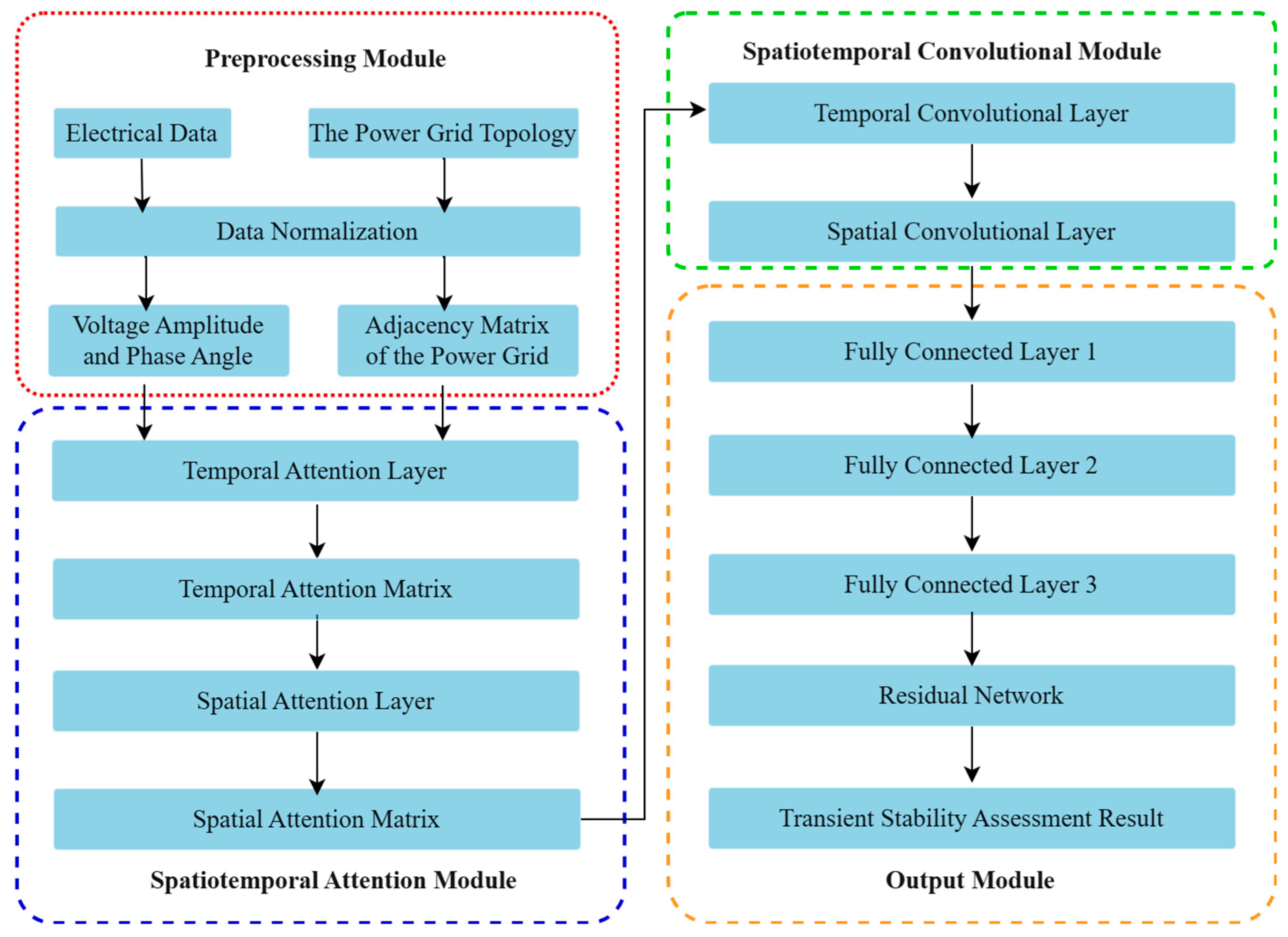
• To address the limitation of existing models in feature extraction, we introduce attention mechanisms in both temporal and spatial dimensions to accurately capture dynamic correlations across different times and locations. The spatiotemporal attention module enhances the model’s feature extraction capability, followed by spatial and temporal convolutional layers, which extract spatial features and capture temporal dependencies, respectively. Finally, the residual network and fully connected layers process these features to produce accurate TSA results. The proposed algorithm offers distinct advantages: The integration of spatiotemporal attention mechanisms significantly improves the model’s ability to focus on critical features, while the combination of convolutional layers and residual networks ensures efficient feature extraction and prevents overfitting, leading to better generalization performance. Additionally, the overall architecture is designed to handle complex spatiotemporal data effectively, making it highly adaptable to various power system scenarios.
• Comprehensive case studies performed on the New England 10-machine 39-bus system and the NPCC 48-machine 140-bus system validate the effectiveness of the proposed methodology.

The remainder of this paper is organized as follows: Section 1 provides a detailed exposition of the proposed ASTGCN. Section 2 outlines the systematic implementation workflow of the ASTGCN-based TSA method. Section 3 presents comprehensive case studies and the discussion. Finally, Section 4 concludes the whole paper.

2. Attention-Based Spatial–Temporal Graph Convolutional Network (ASTGCN)

The transient process in power systems is inherently a dynamic transition from a steady state to a new operational condition, during which physical quantities such as generator rotor angles, voltage magnitudes, and current phasors show significant time-varying characteristics. On the other hand, power systems are structured as graph-based networks, with generator units and substation bus nodes interconnected through transmission lines. This topological configuration fundamentally governs the system-wide distribution of energy and the pathways of energy transfer, thereby exerting a significant impact on transient stability. Therefore, this paper proposes an ASTGCN model, whose architectural framework is schematically depicted in Figure 1. The assessment model is primarily divided into two parts: (1) Spatiotemporal Attention Module: This module employs dual attention mechanisms—temporal attention and spatial attention—to effectively capture dynamic correlations within time-series data of transient processes. (2) Spatiotemporal Convolutional Module: The spatial features of the power network are extracted through a spatial convolutional layer, while the temporal characteristics during transient processes are captured by a temporal convolutional layer. The integrated spatiotemporal features are then fed into fully connected layers, culminating in a Softmax layer that generates the final transient stability classification results.

2.1. Spatiotemporal Attention Module

The attention mechanism originated in the 1980s and was later introduced into the field of deep learning in 2014, gradually becoming a research hotspot in areas such as image classification and machine translation. The core idea is to enable the model to dynamically assign appropriate weights to different parts of the input data, allowing the model to focus more effectively on the most relevant parts of the task, thus enhancing both performance and efficiency. Given the complex spatiotemporal characteristics of transient stability data, this section proposes a spatiotemporal attention module to capture the highly correlated features of spatiotemporal evolution patterns in transient stability data. The spatiotemporal attention module consists of two components: a spatial attention layer and a temporal attention layer.

• spatial attention layer

In the spatial dimension, this paper employs a spatial attention mechanism to describe the spatial dependencies between the features of different nodes in the power grid. The spatial attention mechanism is defined as

$$\mathit{S}={\mathit{V}}_s·\sigma \left(\right({\mathit{X}}_h^{t-1}{\mathit{Q}}_1){\mathit{Q}}_2{({\mathit{Q}}_3{\mathit{X}}_h^{t-1})}^{\mathrm{T}}+{\mathit{b}}_s)$$

(1)

$$S_{i,j}^{\prime }={\displaystyle \frac{exp\left(S_{i,j}\right)}{{\displaystyle {\sum }_{j=1}^{N}exp\left(S_{i,j}\right)}}}$$

(2)

where $\mathit{S}$ denotes the spatial attention matrix; ${\mathit{X}}_h^{t-1}$ denotes the input to the t-th spatiotemporal block; the parameters ${\mathit{V}}_s$, ${\mathit{b}}_s$, ${\mathit{Q}}_1$, ${\mathit{Q}}_2$, and ${\mathit{Q}}_3$ are all learnable network parameters; and $N$ is the total number of nodes. $\sigma$ is the activation function; the element $S_{i,j}$ quantifies the spatial correlation strength between node $i$ and node $j$; the matrix $S_{i,j}^{\prime }$ represents the normalized spatial correlation degrees of $S_{i,j}$.

• temporal attention layer

Since transient stability data exhibit certain correlations across different time segments, with varying degrees of correlation between these segments, this paper employs a temporal attention mechanism to capture the dynamic temporal correlations between transient stability data. The temporal attention mechanism is described as

$$\mathit{W}={\mathit{V}}_r·\sigma \left(\right({\mathit{X}}_h^{t-1}{\mathit{U}}_1){\mathit{U}}_2{({\mathit{U}}_3{\mathit{X}}_h^{t-1})}^{\mathrm{T}}+{\mathit{b}}_r)$$

(3)

$$W_{i,j}^{\prime }={\displaystyle \frac{exp\left(W_{i,j}\right)}{{\displaystyle {\sum }_{j=1}^{N}exp\left(W_{i,j}\right)}}}$$

(4)

where the matrix $\mathit{W}$ denotes the temporal correlation matrix; the parameters ${\mathit{V}}_r$, ${\mathit{b}}_r$, ${\mathit{U}}_1$, ${\mathit{U}}_2$, and ${\mathit{U}}_3$ are all learnable network parameters; the element $W_{i,j}$ quantifies the temporal correlation strength between time steps $i$ and $j$; and the matrix $W_{i,j}^{\prime }$ represents the temporal correlation degrees of $W_{i,j}$ after normalization.

2.2. Spatiotemporal Convolutional Module

After the feature extraction by the spatial and temporal attention layers, the valuable spatiotemporal data from the transient stability data are extracted and then input into the spatiotemporal convolution module, which is similarly divided into spatial and temporal convolution layers.

• Spatial Convolutional Layer

Traditional CNNs are primarily designed for processing Euclidean space data and excel at extracting features from two-dimensional tensor data. However, they struggle to model power network topology and fail to account for the impact of topological connectivity on system stability. To address this limitation, this paper employs spectral convolutional methods in the spatial dimension to exploit neighborhood information between nodes in power networks.

The power system network topology is abstracted as a graph structure, where the Laplacian matrix in the spectral domain is employed to characterize the structural features of the topological graph:

$$\mathit{L}=\mathit{D}-\mathit{A}$$

(5)

where $\mathit{D}$ represents the degree matrix of the power grid topology, and $\mathit{A}$ represents the adjacency matrix of the power grid topology.

By normalizing the Laplacian matrix, the structural characteristics of the power network topology can be redefined as follows:

$$\mathit{L}=\mathit{E}-{\mathit{D}}^{-\frac{1}{2}}\mathit{A}{\mathit{D}}^{-\frac{1}{2}}$$

(6)

where $\mathit{E}$ represents the identity matrix.

The eigenvalue decomposition of the Laplacian matrix is given by the following formula:

$$\mathit{L}=\mathit{U}\mathbf{\Lambda }{\mathit{U}}^{\mathit{T}}$$

(7)

where $\mathit{U}$ is the matrix formed by the unit eigenvectors and $\mathit{U}{\mathit{U}}^{\mathrm{T}}=E$; the diagonal matrix $\mathit{\Lambda }=\left[{\lambda }_1,{\lambda }_2,\dots ,{\lambda }_n\right]$ consists of the eigenvalues of the Laplacian matrix $\mathit{L}$; and $n$ denotes the total number of features.

Based on the Laplacian matrix $\mathit{L}$, the graph convolution formula is defined as follows:

$$(\mathit{X}\mathbf{\ast }\mathit{g})=\mathit{g}\left(\mathit{U}\mathbf{\Lambda }{\mathit{U}}^{\mathrm{T}}\right)\mathit{X}=\mathit{U}\mathit{g}\mathbf{\Lambda }{\mathit{U}}^{\mathrm{T}}\mathit{X}$$

(8)

where $\mathit{X}$ denotes the input feature vector; $\mathbf{\ast }$ represents the graph convolution computation; and $\mathit{g}$ is the filter.

However, the exact computation of $\mathit{g}\mathbf{\Lambda }$ incurs high computational complexity, which increases the time consumption of the model. To accelerate computation, Chebyshev polynomials are introduced to approximate the convolution kernel, leading to an improved convolution formula. The Chebyshev polynomial is defined as follows:

$${\mathit{g}}_{\mathit{\theta }}(\mathit{\Lambda })\mathbf{\approx }{\displaystyle \sum _{H=0}^{H-1}{\theta }_H{T}_H\left(\mathit{\Lambda }\right)}$$

(9)

where ${\theta }_H$ denotes the coefficients of the Chebyshev polynomial, and $T_H\left(x\right)$ represents the Chebyshev polynomial of order H, which is defined as follows:

$$T_H(x)=2x{T}_{H-1}(x)-T_{H-2}(x)$$

(10)

where $T_0\left(x\right)=1$, $T_1\left(x\right)=x$.

Since the Chebyshev polynomials are defined as

$$T_k\left(x\right)=\mathit{cos}\left[k\mathit{arccos}\right(x\left)\right]$$

(11)

The eigenvalue matrix $\mathit{\Lambda }$ needs to be normalized to [−1, 1], and then

$$\tilde{\mathit{\Lambda }}=(2/{\mathit{\lambda }}_{\max })\mathit{\Lambda }-\mathit{E}$$

(12)

where $\tilde{\mathit{\Lambda }}$ denotes the scaled eigenvector matrix, and ${\lambda }_{\max }$ represents the maximum eigenvalue of the Laplacian matrix $\mathit{L}$. By substituting the Chebyshev polynomial approximation for the convolution kernel, Equation (9) is incorporated into Equation (8), yielding the following expression:

$$(\mathit{X}\mathbf{\ast }\mathit{g})=\mathit{g}(\mathit{U}\mathit{\Lambda }{\mathit{\Lambda }}^{\mathrm{T}})\mathit{X}=\mathit{U}\left[{\displaystyle \sum _{H=0}^{H-1}{\theta }_H{T}_H\left(\tilde{\mathit{\Lambda }}\right)}\right]{\mathit{U}}^{\mathrm{T}}\mathit{X}$$

(13)

By leveraging the transformation technique, the matrix operations are embedded into the Chebyshev polynomials, allowing Equation (13) to be reformulated as follows:

$$(\mathit{X}\mathbf{\ast }\mathit{g})={\displaystyle \sum _{H=0}^{H-1}{\theta }_H{T}_H\left(\mathit{U}\tilde{\mathit{\Lambda }}{\mathit{U}}^{\mathrm{T}}\right)}\mathit{X}$$

(14)

$$(\mathit{X}\mathbf{\ast }\mathit{g})={\displaystyle \sum _{H=0}^{H-1}{\theta }_H{T}_H\left(\tilde{\mathit{L}}\right)}\mathit{X}$$

(15)

To dynamically adjust the correlations between nodes, the Chebyshev polynomials are integrated with the spatiotemporal correlation strength matrix $S^{\prime }$ (where each element is denoted as $S_{i,j}^{\prime }$). The final graph convolution formula is derived as follows:

$$\mathit{g}\ast x={\displaystyle \sum _{H=0}^{H-1}{\theta }_H\left(T_H\right(\tilde{\mathit{L}})\otimes S^{\prime })x}$$

(16)

where $\otimes$ denotes the Hadamard product.

• Temporal Convolutional Layer

The spatial convolutional layer has already captured the neighborhood information of each node in the power network topology along the spatial dimension. The temporal convolutional layer is applied to further aggregate information from adjacent time steps. The formula for the temporal convolutional layer is described as follows::

$${\mathit{X}}_h^t=RELU(\phi \ast (RELU(\mathit{g}\ast {\mathit{X}}_h^{t-1}\left)\right))$$

(17)

where $\phi$ denotes the parameters of the convolutional kernel along the temporal dimension, and $RELU(\cdot )$ represents the activation function.

3. The TSA Method Based on the ASTGCN

When the power system faces transient instability risks, it is essential to quickly and accurately identify the transient stability status, enabling timely and effective adjustments to operational strategies. To achieve this, electrical measurement data from various nodes and the topological connection relationships are required for real-time monitoring of the system’s operational state. Additionally, the spatiotemporal attention convolutional model developed in Section 1 is employed to transform the transient stability prediction task into a binary classification task, thereby determining the system’s stable operating condition post-fault.

3.1. Model Input and Output

The rationality of input feature construction critically impacts the model’s assessment performance. Power system transient processes exhibit dynamic characteristics in the temporal dimension and graph-domain topological properties in the spatial dimension. To improve the accuracy of TSA, it is necessary to comprehensively consider the spatiotemporal distribution characteristics of transients and construct input features for the TSA model from both temporal and spatial perspectives. In terms of temporal features, the variations in voltage magnitude and voltage phase angle during the transient process of the power system can intuitively reflect the system’s response characteristics and are closely related to transient stability. Therefore, the voltage magnitudes and phase angles of all nodes during pre-fault, during-fault, and post-fault periods are selected as the temporal input features. The total number of sampling points is denoted as $N_u$, the sampling interval as $T_{\mathrm{g}}$, and the sampling range as $[t_0-T_{\mathrm{g}},t_e-w{T}_{\mathrm{g}}]$. Here, $t_0$ represents the fault occurrence time, $t_{\mathrm{e}}$ is the fault clearance time, and $w$ is the number of sampling points after fault clearance. Therefore, the input data for the system voltage magnitude and phase angle $\theta$ are as follows:

$$U=\left[\begin{array}{cccc}{U}_{1,1}& U_{1,2}& \cdots & U_{1,N_u}\\ U_{2,1}& U_{2,2}& \cdots & U_{2,N_u}\\ ⋮& ⋮& & ⋮\\ U_{n,1}& U_{n,2}& \cdots & U_{n,N_u}\end{array}\right]$$

(18)

$$\theta =\left[\begin{array}{cccc}{\theta }_{1,1}& {\theta }_{1,2}& \cdots & {\theta }_{1,N_u}\\ {\theta }_{2,1}& {\theta }_{2,2}& \cdots & {\theta }_{2,N_u}\\ ⋮& ⋮& & ⋮\\ {\theta }_{n,1}& {\theta }_{n,2}& \cdots & {\theta }_{n,N_u}\end{array}\right]$$

(19)

where $U$ and $\theta$ represent the voltage magnitude and phase angle matrices, respectively, and $n$ denotes the number of nodes in the power system.

In terms of spatial features, to account for the influence of topological connectivity on power transmission paths and distribution, and to capture the spatial evolution patterns of the system, the adjacency matrix of the system topology is incorporated into the model input to consider the dynamic interactions between nodes.

The output is a set of labels corresponding one-to-one with the input samples. In this paper, the output of the TSA task includes two categories: stable or unstable, which can be represented as follows:

$${\widehat{y}}_i={\displaystyle \frac{exp\left(z_i\right)}{{\displaystyle {\sum }_{j=0}^1\mathit{exp}\left(z_j\right)}}}$$

(20)

where ${\widehat{y}}_i$ represents the output of the $i$-th predicted category, and $z_i$ denotes the input of the $i$-th predicted category. After normalization using the Softmax function in Equation (20), the result will be ${\widehat{y}}_i\in [0,1]$ and ${\displaystyle \sum {\widehat{y}}_i=1}$.

For the sample dataset obtained through time-domain simulation methods, this paper introduces the Transient Stability Index (TSI) to assess whether the system will experience rotor angle instability under large disturbances. The definition of TSI is as follows:

$$I_{\mathrm{TSI}}={\displaystyle \frac{\Theta -|\Delta {\delta }_{max}|}{\Theta +|\Delta {\delta }_{max}|}}$$

(21)

where $\Theta ={360}^{\circ }$, and $\Delta {\delta }_{\max }$ represents the maximum rotor angle difference among generators. When $I_{\mathrm{TSI}}>0$, the sample is stable and labeled as (1,0); otherwise, the sample is unstable and labeled as (0,1).

3.2. Adaptive Focal Loss Function

The loss function, also known as the cost function, is primarily used to evaluate the degree of discrepancy between the model’s predicted values and the actual values. In classification tasks, the cross-entropy loss function is typically chosen to guide model training, and its formula is

$$L_{CE}=-[y\mathit{log}\widehat{y}+(1-y\left)\mathit{log}\right(1-\widehat{y}\left)\right]$$

(22)

where $y$ represents the true target value, i.e., the transient stability label of the sample, and $\widehat{y}$ represents the predicted output from the model. It can be seen that the value $C_E$ decreases as $y$ and $\widehat{y}$ become closer.

In power system TSA, transient instability events are rare, leading to imbalanced datasets and increasing the risk of misclassifying instability. To address the issue of sample imbalance, the focal loss optimizes and improves the traditional cross-entropy loss function [26]. On one hand, a weight factor $\alpha$ ($\alpha \in [0,1]$) is introduced to balance the loss weights of stable and unstable samples. On the other hand, a focusing factor $\gamma$ ($\gamma \in \left[0,+\infty \right.)$) is introduced to adjust the loss weights of samples with different difficulty levels. Ultimately, the focal loss is defined as follows:

$$L_{FL}=-\alpha {(1-\widehat{y})}^{\gamma }\mathit{log}\widehat{y}$$

(23)

Although the function $L_{FL}$ can improve the performance of single-stage algorithms in the face of sample imbalance issues, it is inherently a static loss function, meaning both $\alpha$ and $\gamma$ are hyperparameters. However, during the training process of the model, both the inter-class imbalance of samples and the learning difficulty degree of samples may change, requiring extensive tuning of $\alpha$ and $\gamma$, which consumes excessive computational resources. To address the aforementioned issues, this paper proposes an adaptive focal loss function $L_{AFL}$, which introduces an adaptive weight factor ${\alpha }^{\prime }$ and an adaptive focusing factor ${\gamma }^{\prime }$ based on the focal loss function.

• Adaptive Weight Factor

To enable the loss function to dynamically balance inter-class samples by adjusting the loss weights of different categories across various datasets, an adaptive weight factor ${\alpha }^{\prime }$ is designed. This factor is determined using a heuristic method, which rescales the loss weights based on the number of samples in each category. The purpose is to assign a larger weight factor to classes with fewer samples and maintain a weight factor around 1 for classes with abundant samples. The adaptive weight factor ${\alpha }^{\prime }$ is defined as follows:

$${\alpha }^{\prime }=\left\{\begin{array}{cc}{\displaystyle \frac{{\alpha }_0(n_i+N)}{N}}\times (-\log ({\displaystyle \frac{n_i}{N}}\left)\right),\hfill & y=1\hfill \\ {\displaystyle \frac{(1-{\alpha }_0)N-{\alpha }_0{n}_i}{N}}\times (-\log ({\displaystyle \frac{n_i}{N}}),\hfill & y=0\hfill \end{array}\right.$$

(24)

where ${\alpha }^{\prime }$ is the initialization coefficient of the weight factor; $n_i$ is the number of samples in the $i$-th class; and $N$ is the total number of samples. The adaptive weight factor ${\alpha }^{\prime }$ can dynamically adjust the loss weights of inter-class samples based on the imbalanced sample quantities in different datasets.

• Adaptive Focusing Factor

Although the adaptive weight factor ${\alpha }^{\prime }$ is designed to address the issue of inter-class sample imbalance, it mitigates the negative impact of imbalanced samples to some extent. However, during the training process, the model’s feature extraction capability gradually improves, and the classification of easy and hard samples will change, meaning that the model gains better recognition ability for samples initially assessed as difficult. To address this, an adaptive focusing factor ${\gamma }^{\prime }$ is designed. It rebalances the loss weights of different samples based on their difficulty levels, thereby reducing the impact of samples with varying difficulty on the convergence process of the deep learning model. The adaptive focusing factor ${\gamma }^{\prime }$ is defined as follows:

$${\gamma }^{\prime }={\displaystyle \frac{{\gamma }_0}{log(E-1+e)}}$$

(25)

where ${\gamma }_0$ is the initial focusing factor, and $E$ is the total number of training iterations for the model.

• Adaptive Focal Loss Function

Based on the adaptive weight factor ${\alpha }^{\prime }$ and the adaptive focusing factor ${\gamma }^{\prime }$, the adaptive focal loss function $L_{AFL}$ is derived as follows:

$$L_{AFL}=-{\alpha }^{\prime }{(1-\widehat{y})}^{{\gamma }^{\prime }}\mathit{log}\widehat{y}$$

(26)

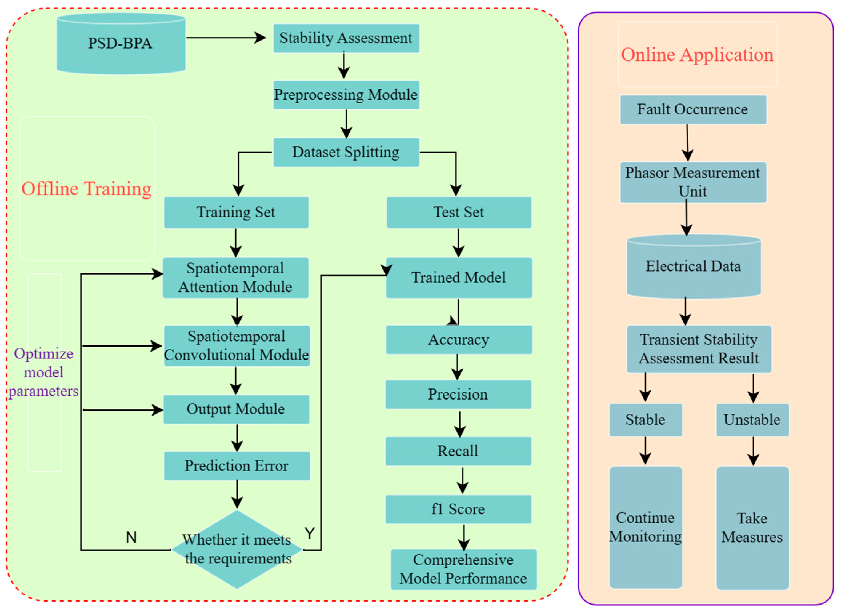
3.3. The TSA Process

The TSA process based on the ASTGCN is illustrated in Figure 2, which is divided into two phases: offline training and online application. The specific steps are as follows:

• Simulation Data Generation: A large amount of simulation data is generated using the PSD-BPA 4.5.3 time-domain simulation software, with the richness and diversity of the sample data improved by varying load levels, fault locations, and load compositions.
• Transient Stability Classification of Samples: Based on the transient stability evaluation criteria for power systems and combined with the simulation data, the transient stability status of the samples is classified.
• Input Feature Processing: Voltage magnitudes and phase angles of each node are extracted from the generated simulation data to construct the input features.
• Model Training: The ASTGCN model is trained in a forward manner using the training set, and its parameters are optimized in reverse based on the adaptive focal loss function.
• Model Testing: The test set is fed into the trained ASTGCN model for evaluation, and the model’s assessment performance is comprehensively evaluated based on the test results.
• Online Application: Online operational data is collected and processed, and by utilizing the trained ASTGCN model, fast and accurate assessment of transient stability is achieved. If the assessment indicates that the system is unstable, immediate emergency control measures must be taken to prevent further deterioration of the system. For instance, generator tripping can be implemented to rapidly reduce the system’s generation power, thereby balancing the power imbalance. Additionally, load shedding can be carried out to alleviate the system’s load pressure and swiftly restore system stability.

3.4. Evaluation Metrics

The performance of different models is comprehensively evaluated using four evaluation metrics: accuracy $A_{\mathrm{cc}}$, precision $P_{\mathrm{rec}}$, recall $R_{\mathrm{ec}}$, and ${\mathrm{f}}_1$-score. Their formulas are as follows:

$$A_{\mathrm{cc}}={\displaystyle \frac{T_{\mathrm{P}}+T_{\mathrm{N}}}{T_{\mathrm{P}}+T_{\mathrm{N}}+F_{\mathrm{P}}+F_{\mathrm{N}}}}$$

(27)

$$P_{\mathrm{rec}}={\displaystyle \frac{T_{\mathrm{P}}}{T_{\mathrm{P}}+F_{\mathrm{P}}}}$$

(28)

$$R_{\mathrm{ec}}={\displaystyle \frac{T_{\mathrm{P}}}{F_{\mathrm{N}}+T_{\mathrm{P}}}}$$

(29)

$${\mathrm{f}}_1=2\times {\displaystyle \frac{P_{\mathrm{rec}}\times R_{\mathrm{ec}}}{P_{\mathrm{rec}}+R_{\mathrm{ec}}}}$$

(30)

where $T_{\mathrm{P}}$ represents the number of samples predicted as positive by the model that are actually positive; $T_{\mathrm{N}}$ represents the number of samples predicted as negative that are actually negative; $F_{\mathrm{P}}$ represents the number of samples predicted as positive that are actually negative; and $F_{\mathrm{N}}$ represents the number of samples predicted as negative that are actually positive.

4. Case Study

To validate the effectiveness of the proposed method, the ASTGCN model is implemented in the PaddlePaddle environment using the Python 3.10 programming language.

4.1. The New England 10-Machine 39-Bus System

4.1.1. Sample Generation

The test system used is the New England 10-machine 39-node system, which consists of 10 generators, 39 buses, and 46 transmission lines. For this system, six different load levels—80%, 85%, 90%, 95%, 100%, and 105%—are considered, and the generator outputs are adjusted accordingly to ensure the convergence of the power flow calculation. Faults are set on transmission lines, where 12 out of 46 lines contain transformers. For the remaining 34 lines, faults are set at locations 0%, 15%, 30%, …, and 90% on each line, resulting in a total of seven different fault locations. The fault type is set to the most severe three-phase short-circuit fault in power systems. The fault clearing times are considered at the 1st cycle, 2nd cycle, …, and 16-th cycle after the fault occurrence, resulting in a total of 15 fault clearing times. The power system simulation software PSD-BPA is used to randomly generate 24,276 samples, including 15,030 stable samples and 9246 unstable samples. The stability state of each sample is determined based on Equation (21), which effectively discriminates between stable and unstable conditions of the system under various disturbances. The training set and test set are randomly divided at a ratio of 4:1. The classification of the sample set is shown in

Table 1. Sample set details.

Sample Set	Total Numbers	Stable Samples	Unstable Samples
Total Samples	24,276	15,030	9246
Training Set	19,420	12,024	7397
Test Set	4856	3006	1849

.

4.1.2. Performance Analysis of the Adaptive Focal Loss Function

The performance metrics of the ASTGCN model trained using the cross-entropy loss function $L_{CE}$, focal loss function $L_{FL}$, and adaptive focal loss function $L_{AFL}$ on the test set are shown in

Table 2. Test results of different loss functions.

Function	${\mathit{A}}_{\mathrm{cc}}$/%	${\mathit{P}}_{\mathrm{rec}}$/%	${\mathit{R}}_{\mathrm{ec}}$/%	${\mathbf{f}}_1$/%
$L_{CE}$	98.52	98.91	97.84	98.37
$L_{FL}$	99.10	99.45	98.65	99.05
$L_{AFL}$	99.38	99.73	98.94	99.32

. The accuracy of function $L_{AFL}$ increased by 0.28% and 0.86% compared to function $L_{FL}$ and function $L_{CE}$, respectively. The reason is that, compared to the traditional cross-entropy loss function, function $L_{AFL}$ effectively mitigates the adverse effects of imbalanced positive and negative samples on model training by introducing an adaptive class weight factor. Compared to function $L_{FL}$, function $L_{AFL}$ introduces dynamic parameters to adjust the model’s focus on hard samples, thereby utilizing data resources more efficiently during training and improving the overall performance of the model.

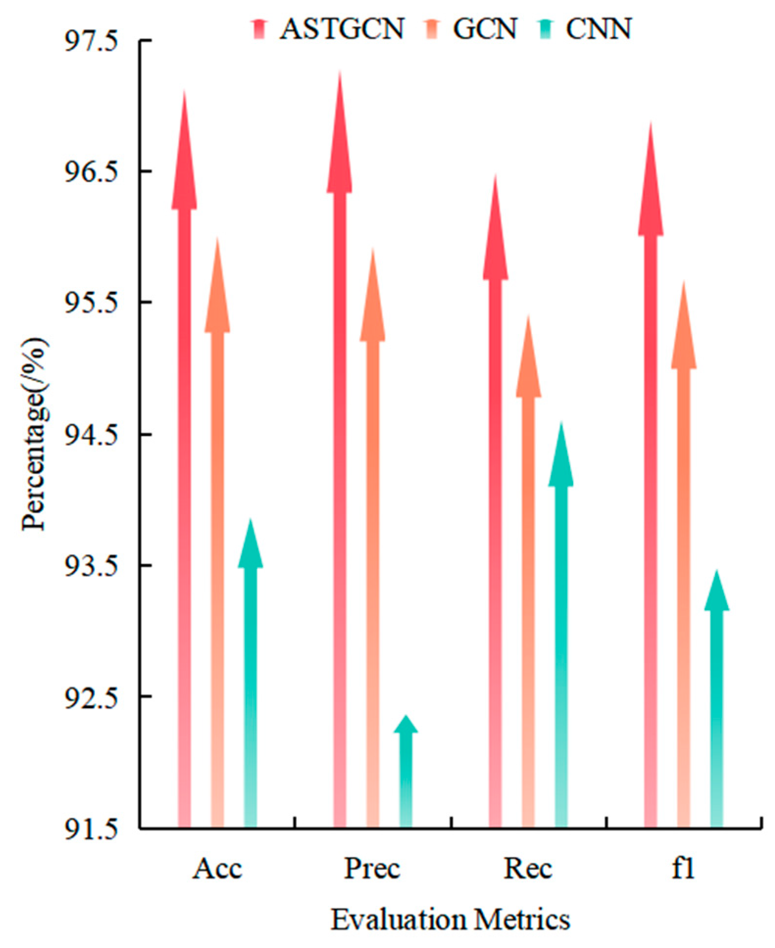
4.1.3. Comparative Evaluation of Model Performance

To validate the performance of the ASTGCN model when applied to TSA, its prediction results are compared to those of SVM, DT, KNN, RF, XGBoost, CNNs, and GCNs. The kernel function of the SVM adopts the radial basis function (RBF), and the DT employs the C 5.0 algorithm. The network structure adopted by the CNN is as follows: input layer, convolutional layer, pooling layer, convolutional layer, pooling layer, two fully connected layers, and the Softmax output layer. The network structure of LSTM consists of two stacked LSTM blocks, two fully connected layers, and a Softmax output layer. The structure of GCN consists of two stacked GCN layers, two fully connected layers, and a Softmax output layer. All the aforementioned deep models are trained using the Adam optimizer with an adaptive focal loss function $L_{AFL}$, where the learning rate is set to 0.001 and the batch size to 150. Additionally, the Chebyshev polynomial order in the ASTGCN is configured to 2. The classification prediction results of the ASTGCN model and other models are shown in

Table 3. Resulting metrics of 8 models.

Model	${\mathit{A}}_{\mathrm{cc}}$/%	${\mathit{P}}_{\mathrm{rec}}$/%	${\mathit{R}}_{\mathrm{ec}}$/%	${\mathbf{f}}_1$/%
ASTGCN	99.38	99.73	98.94	99.32
GCN	98.62	99.18	97.83	98.51
CNN	98.25	97.86	98.38	98.12
DT	95.62	97.45	92.99	95.17
KNN	95.04	97.69	91.37	94.43
XGBoost	94.62	95.15	94.47	94.81
SVM	93.12	97.13	88.71	93.06
RF	92.37	94.48	90.63	92.51

. To account for randomness, all experiments are repeated 15 times, and the average values are taken as the final evaluation results.

As shown in Table 3 and Figure 3, compared to the shallow learning methods such as SVM, DT, KNN, RF, XGBoost, and DT, the deep learning algorithms, the GCN, the CNN, and the proposed ASTGCN, significantly enhance model capacity through their deep architectures, leading to a notable improvement in model identification performance. The SVM and DT algorithms perform poorly due to the influence of dataset scale and high-dimensional features, with accuracy rates both below 96%. The GCN can learn the spatial features of the power grid, and its prediction performance is higher than that of the CNN. However, it fails to fully exploit the spatiotemporal characteristics in the data, resulting in lower prediction performance compared to the ASTGCN model.

4.1.4. Ablation Studies on ASTGCN

To assess the individual impact of spatial and temporal attention modules, ablation studies were conducted as follows:

Ablation Model 1: The spatial attention layer is removed from the model, while all other settings are kept consistent with the ASTGCN model.

Ablation Model 2: The temporal attention layer is removed from the model, while all other settings are kept consistent with the ASTGCN model.

The experimental results in

Table 4. Results of ablation studies.

Model	${\mathit{A}}_{\mathrm{cc}}$/%	${\mathit{P}}_{\mathrm{rec}}$/%	${\mathit{R}}_{\mathrm{ec}}$/%	${\mathbf{f}}_1$/%
Ablation Model 1	99.02	99.18	98.65	98.91
Ablation Model 2	99.13	99.45	98.64	99.05

demonstrate that removing either the spatial attention layer or the temporal attention layer leads to a degradation in model performance.

4.1.5. Analysis of the Impact of Sample Size on Model Performance

To analyze the impact of sample size on the performance of the evaluation model, the number of training set samples is set to 2000, 3000, 4000, and 5000, respectively, while the number of test set samples is fixed at 5000. The ASTGCN, GCN, and CNN models are trained, and the accuracy evaluation results on the test set are shown in Figure 4.

As shown in Figure 4, under training with the same number of samples, the ASTGCN model achieves higher accuracy than the GCN and CNN models. Moreover, for the same test accuracy, the ASTGCN model requires the fewest samples among the three models.

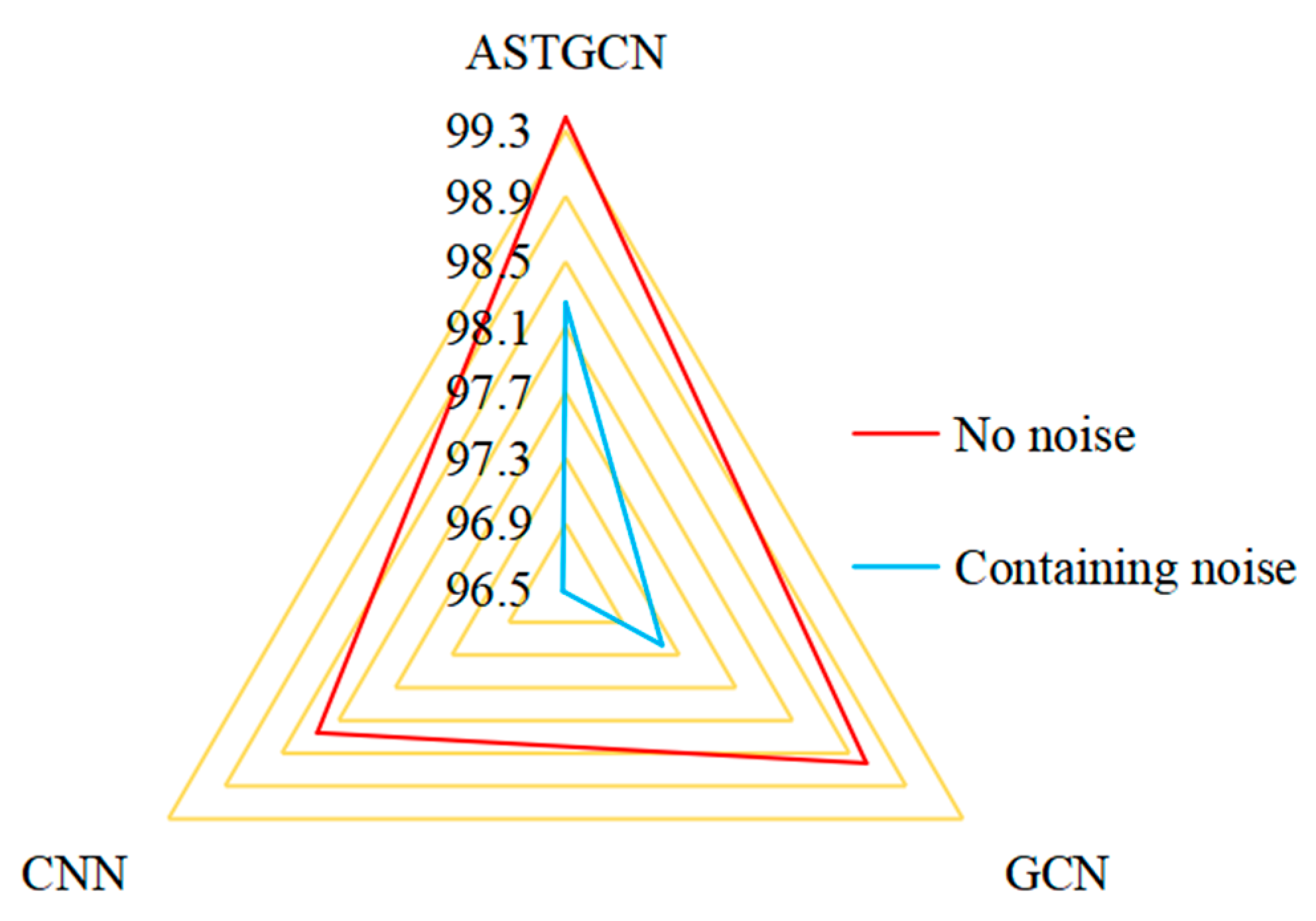
4.1.6. Robustness of the Model to Noise

In practice, errors and noise interference may occur when PMUs sample data from various nodes in the power system. According to the IEEE standard for synchronized phasor data transmission in power systems, the PMU’s phasor measurement error is less than 6.0%. To enhance the model’s robustness to noise, random errors ranging from 0% to 6% are added to all input data in the dataset during both training and testing. The evaluation results of the ASTGCN, GCN, and CNN models under noisy conditions are shown in Figure 5.

It can be observed that, compared to the noise-free scenario, the accuracy of each method is affected to some extent. However, the proposed ASTGCN model in this paper can predict transient stability states with an accuracy of 98.25%, outperforming other methods.

4.1.7. Generalization Performance Under Unknown Topologies

This section verifies the generalization performance of the proposed ASTGCN under topology changes by setting different topologies in the test set compared to the training set. The topology of the test set under the new topology scenario is the N-4 topology (randomly disconnecting four transmission lines and adjusting generator outputs accordingly to ensure the convergence of power flow calculations). This topology is designed to simulate extreme contingencies, such as cascading failures and islanding phenomena. The sample simulation method under each topology is consistent with Section 3.1. Under the above conditions, a large number of simulation samples are randomly generated, totaling 3500 samples, including 2225 unstable samples and 1275 stable samples. The evaluation results of the ASTGCN, GCN, and CNN models on the new dataset are shown in Figure 6.

It can be observed that, under topology changes, the ASTGCN model achieves higher test accuracy than the other two methods. Among them, the GCN model also demonstrates good prediction performance but is 1.12% lower than the ASTGCN model. This is because both the GCN and ASTGCN models extract the spatial characteristics of the power grid. When the system’s topology changes, it is reflected in the input adjacency matrix of the models. However, the ASTGCN model also extracts temporal characteristics, considering the spatiotemporal nature of the data, which is why its performance surpasses that of the GCN. On the other hand, the input of the CNN model does not include any explicit spatial information, making it unable to capture topological changes, leading to reduced evaluation performance on the new topology dataset. Therefore, the proposed ASTGCN model exhibits better generalization performance under new topologies.

4.2. Large-Scale Power Grid Testing

To further validate the effectiveness of the ASTGCN model, a larger-scale NPCC 48-machine, 140-bus system is employed for testing. This system comprises 48 generators, 233 transmission lines, and 140 buses. During the testing process, the load level is set to vary between 75% and 110% of the base load, with an adjustment step size of 5%. The fault type is specified as a three-phase short-circuit fault. The fault lines are selected from transmission lines without transformers. Four different fault clearance times are considered: the 5th, 8th, 11th, and 14th cycles after the fault occurrence. Based on these settings, a total of 15,075 samples are generated, including 7589 stable samples and 7486 unstable samples. The samples are randomly divided into a training set and a testing set, with 11,200 samples allocated to the training set and the remaining 3875 samples to the testing set.

In this study, the ASTGCN model is compared with several other deep learning methods, and the results are presented in

Table 5. Resulting metrics of 3 models.

Model	${\mathit{A}}_{\mathrm{cc}}$/%	${\mathit{P}}_{\mathrm{rec}}$/%	${\mathit{R}}_{\mathrm{ec}}$/%	${\mathbf{f}}_1$
ASTGCN	99.00	99.72	98.11	98.93
GCN	98.36	98.91	97.57	98.24
CNN	98.11	98.63	97.30	97.96

. It can be observed that the ASTGCN model demonstrates superior performance, maintaining high prediction accuracy even in large-scale system scenarios.

5. Conclusions

This paper proposes a novel TSA method based on the ASTGCN model. The contributions and innovations of this method are as follows.

Firstly, to address the issue of sample imbalance, an adaptive focal loss function is designed. By adaptively adjusting the weight coefficients of the loss function, the tendency of the model to classify too many samples as stable during training is mitigated. This allows the model to focus more on misclassified and difficult samples, improving the global accuracy and generalization capability of TSA. Compared with the cross-entropy loss function, the adaptive focal loss function has improved the accuracy by 0.86%

Secondly, to tackle the insufficient feature extraction capability of existing models, a spatiotemporal attention convolutional model is established. This model not only captures the temporal characteristics of transient processes but also incorporates the influence of topological relationships between nodes, effectively enhancing the prediction accuracy of the model. Compared to the GCN model, ASTGCN has improved the accuracy by 0.76%.

Additionally, the superiority of the proposed method is validated on the New England 10-machine 39-bus system and the NPCC 48-machine 140-bus system.

In summary, the ASTGCN model proposed in this paper is primarily designed for offline and online analysis scenarios based on simulation analysis. It demonstrates high accuracy, effectively shortens simulation time, and enhances the efficiency of analysis. In future research, we will focus on addressing the challenges of network topology maintenance and limited measurement information in certain online analysis scenarios. Moreover, we will further adapt and refine the ASTGCN model to improve its applicability across a broader range of online analysis contexts. Additionally, we plan to extend the application of this model to the assessment of voltage stability and frequency stability, broadening its utility in power system analysis.

References

1. Jiang, H.; Wang, K.; Wang, Y.; Gao, M.; Zhang, Y. Energy big data: A survey. IEEE Access 2016, 4, 3844–3861. [Google Scholar] [CrossRef]
2. Zadkhast, P.; Jatskevich, J.; Vaahedi, E. A Multi-Decomposition Approach for Accelerated Time-Domain Simulation of Transient Stability Problems. IEEE Trans. Power Syst. 2015, 30, 2301–2311. [Google Scholar] [CrossRef]
3. Vu, T.L.; Turitsyn, K. Lyapunov Functions Family Approach to Transient Stability Assessment. IEEE Trans. Power Syst. 2016, 31, 1269–1277. [Google Scholar] [CrossRef]
4. Ashraf, S.M.; Gupta, A.; Choudhary, D.K.; Chakrabarti, S. Voltage stability monitoring of power systems using reduced network and artificial neural network. Int. J. Electr. Power Energy Syst. 2017, 87, 43–51. [Google Scholar] [CrossRef]
5. Guo, T.; Milanović, J.V. Probabilistic Framework for Assessing the Accuracy of Data Mining Tool for Online Prediction of Transient Stability. IEEE Trans. Power Syst. 2014, 29, 377–385. [Google Scholar] [CrossRef]
6. Gomez, F.R.; Rajapakse, A.D.; Annakkage, U.D.; Fernando, I.T. Support Vector Machine-Based Algorithm for Post-Fault Transient Stability Status Prediction Using Synchronized Measurements. IEEE Trans. Power Syst. 2011, 26, 1474–1483. [Google Scholar] [CrossRef]
7. Kamwa, I.; Samantaray, S.R.; Joos, G. Catastrophe predictors from ensemble decision-tree learning of wide-area severity indices. IEEE Trans. Smart Grid 2010, 1, 144–158. [Google Scholar] [CrossRef]
8. Wang, L.; Lyu, F.; Su, Y.; Yue, J. Kernel Entropy-Based Classification Approach for Super buck Converter Circuit Fault Diagnosis. IEEE Access 2018, 6, 45504–45514. [Google Scholar] [CrossRef]
9. Pannell, Z.; Ramachandran, B.; Snider, D. Machine learning approach to solving the transient stability assessment problem. In Proceedings of the 2018 IEEE Texas Power and Energy Conference (TPEC), College Station, TX, USA, 14–17 January 2018; pp. 1–6. [Google Scholar]
10. Wang, N.; Ma, Z.; Huo, P.; Liu, X. Predicting Crop Yield Using 3D Convolutional Neural Network with Dimension Reduction and Metric Learning. In Proceedings of the 2023 IEEE 6th International Conference on Pattern Recognition and Artificial Intelligence (PRAI), Haikou, China, 18–20 August 2023; pp. 1004–1008. [Google Scholar]
11. Dong, Q.; Ge, F.; Ning, Q.; Zhao, Y.; Lv, J.; Huang, H.; Yuan, J.; Jiang, X.; Shen, D.; Liu, T. Modeling Hierarchical Brain Networks via Volumetric Sparse Deep Belief Network. IEEE Trans. Biomed. Eng. 2020, 67, 1739–1748. [Google Scholar] [CrossRef] [PubMed]
12. Bang, S.S.; Kwon, G.-Y. Anomaly Detection for HTS Cable Using Stacked Autoencoder and Reflectometry. IEEE Trans. Appl. Supercond. 2023, 33, 1–5. [Google Scholar] [CrossRef]
13. Quan, Z.; Zeng, W.; Li, X.; Liu, Y.; Yu, Y.; Yang, W. Recurrent Neural Networks with External Addressable Long-Term and Working Memory for Learning Long-Term Dependences. IEEE Trans. Neural Netw. Learn. Syst. 2020, 31, 813–826. [Google Scholar] [CrossRef] [PubMed]
14. Shi, Z.; Yao, W.; Zeng, L.; Wen, J.; Fang, J.; Ai, X.; Wen, J. Convolutional neural network-based power system transient stability assessment and instability mode prediction. Appl. Energy 2020, 263, 114586. [Google Scholar] [CrossRef]
15. Yu, J.J.Q.; Hill, D.J.; Lam, A.Y.S.; Gu, J.; Li, V.O.K. Intelligent time-adaptive transient stability assessment system. IEEE Trans. Power Syst. 2018, 33, 1049–1058. [Google Scholar] [CrossRef]
16. Lu, Z.; Shi, X.; He, C.; Wang, X.; Zhou, B. Transient Stability Assessment Based on Two-Step Improved One-Dimensional Convolutional Neural Networks with Long and Short Time-Series Input. In Proceedings of the 2023 International Conference on Power System Technology (PowerCon), Jinan, China, 21–22 September 2023; pp. 1–5. [Google Scholar]
17. Wu, S.; Zheng, L.; Hu, W.; Yu, R.; Liu, B. Improved Deep Belief Network and Model Interpretation Method for Power System Transient Stability Assessment. J. Mod. Power Syst. Clean Energy 2020, 8, 27–37. [Google Scholar] [CrossRef]
18. Wang, X.; Zhou, Q.; Huang, C.; Liao, S.; Jiang, Y.; Ge, Y. A Transient Stability Assessment Method Using LSTM Network with Attention Mechanism. In Proceedings of the 2019 IEEE 8th International Conference on Advanced Power System Automation and Protection (APAP), Xi’an, China, 21–24 October 2019; pp. 120–124. [Google Scholar]
19. Ramirez-Gonzalez, M.; Sevilla, F.R.S.; Korba, P.; Castellanos, R. CNN with squeeze and excitation attention module for power system transient stability assessment. In Proceedings of the 2024 12th International Conference on Smart Grid (icSmartGrid), Setubal, Portugal, 27–29 May 2024; pp. 475–479. [Google Scholar]
20. Hu, W.; Li, X.; Zhao, Y.; Zhang, Y.; Chen, L.; Wang, Z.; Zhou, H. An Updated Method of Transient Stability Assessment Rules for Power Systems in Variable Topology Scenarios Based on Double-Layer Heterogeneous Graph Attention Network. In Proceedings of the 2023 6th Asia Conference on Energy and Electrical Engineering (ACEEE), Chengdu, China, 21–23 July 2023; pp. 222–228. [Google Scholar]
21. Xia, S.; Zhang, C.; Li, Y.; Li, G.; Ma, L.; Zhou, N.; Zhu, Z.; Ma, H. GCN-LSTM Based Transient Angle Stability Assessment Method for Future Power Systems Considering Spatial-Temporal Disturbance Response Characteristics. Prot. Control Mod. Power Syst. 2024, 9, 108–121. [Google Scholar] [CrossRef]
22. Huang, J.; Guan, L.; Su, Y.; Yao, H.; Guo, M.; Zhong, Z. A topology adaptive high-speed transient stability assessment scheme based on multigraph attention network with residual structure. Int. J. Electr. Power Energy Syst. 2021, 130, 106948. [Google Scholar] [CrossRef]
23. Shao, C.; He, X.; Ma, L.; Wang, H.; Zhou, C.; Dong, H. Transient Assessment of Power Systems Based on Graph Attention Networks. In Proceedings of the 2024 IEEE 5th International Conference on Advanced Electrical and Energy Systems (AEES), Lanzhou, China, 29 November–1 December 2024; pp. 525–530. [Google Scholar]
24. Huangfu, H.; Wang, Y.; Lin, H. Power System Transient Stability Assessment Method Based on Optimized Time-Spectral Graphical Neural Network. In Proceedings of the 2024 Boao New Power System International Forum—Power System and New Energy Technology Innovation Forum (NPSIF), Qionghai, China, 8–10 December 2024; pp. 763–767. [Google Scholar]
25. Huang, J.; Guan, L.; Cai, Z.; Chen, L.; Chen, H.; Chen, Z. A Global Attention Pooling-Based Graph Learning Scheme for Generator-Level Transient Stability Assessment. In Proceedings of the 2023 IEEE Power & Energy Society General Meeting (PESGM), Orlando, FL, USA, 16–20 July 2023; pp. 1–5. [Google Scholar]
26. Lin, T.Y.; Goyal, P.; Girshick, R.; He, K.; Dollár, P. Focal Loss for Dense Object Detection. IEEE Trans. Pattern Anal. Mach. Intell. 2017, 42, 2999–3007. [Google Scholar]
Figure 1. The whole framework of the ASTGCN.
Energies 18 03824 g001
Figure 2. The TSA process.
Energies 18 03824 g002
Figure 3. Comparison of metrics of 8 models.
Energies 18 03824 g003
Figure 4. Accuracy results of 3 models under different training set sample sizes.
Energies 18 03824 g004
Figure 5. Accuracy of each model under noise conditions.
Energies 18 03824 g005
Figure 6. Generalization accuracy of each model under new topologies.
Energies 18 03824 g006