
A Method for Selecting the Appropriate Source Domain Buildings for Building Energy Prediction in Transfer Learning: Using the Euclidean Distance and Pearson Coefficient


Abstract
1. Introduction
2. Background
2.1. Pearson Correlation Coefficient and Euclidean Distance
2.2. Transfer Learning
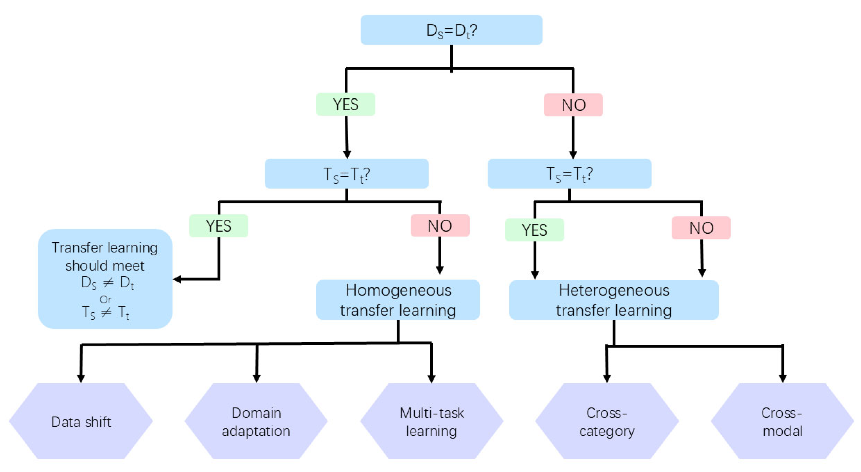
2.2.1. Classifications of Transfer Learning
- Task relationships
- Detailed implementation
- Technical application
2.2.2. Transfer Learning in Building Energy Prediction
2.2.3. Source Domain Selection Method
2.3. Black-Box (Data-Driven Method)
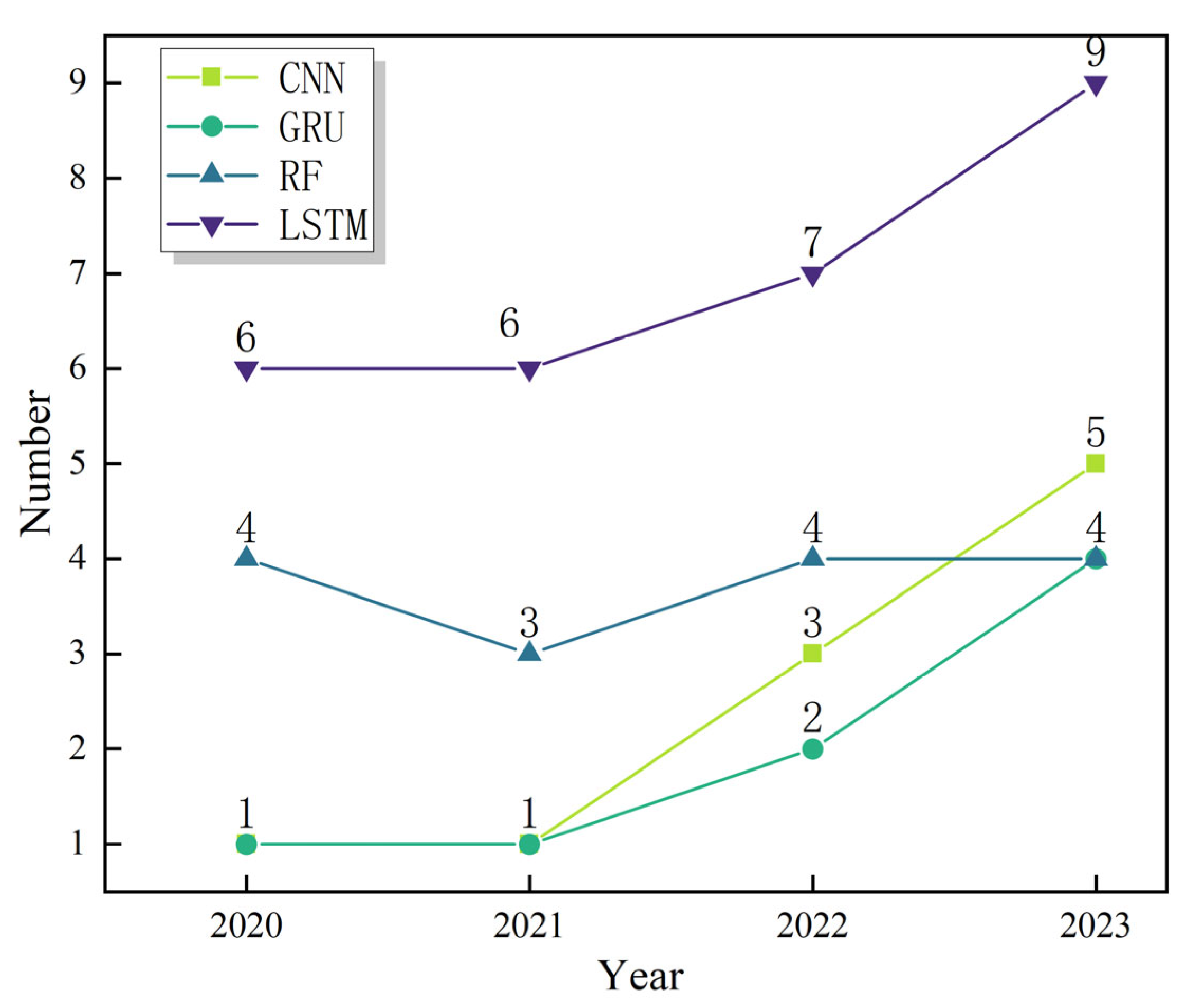
2.3.1. Data-Driven Method Applications for Building Energy Prediction: From Machine Learning to Deep Learning
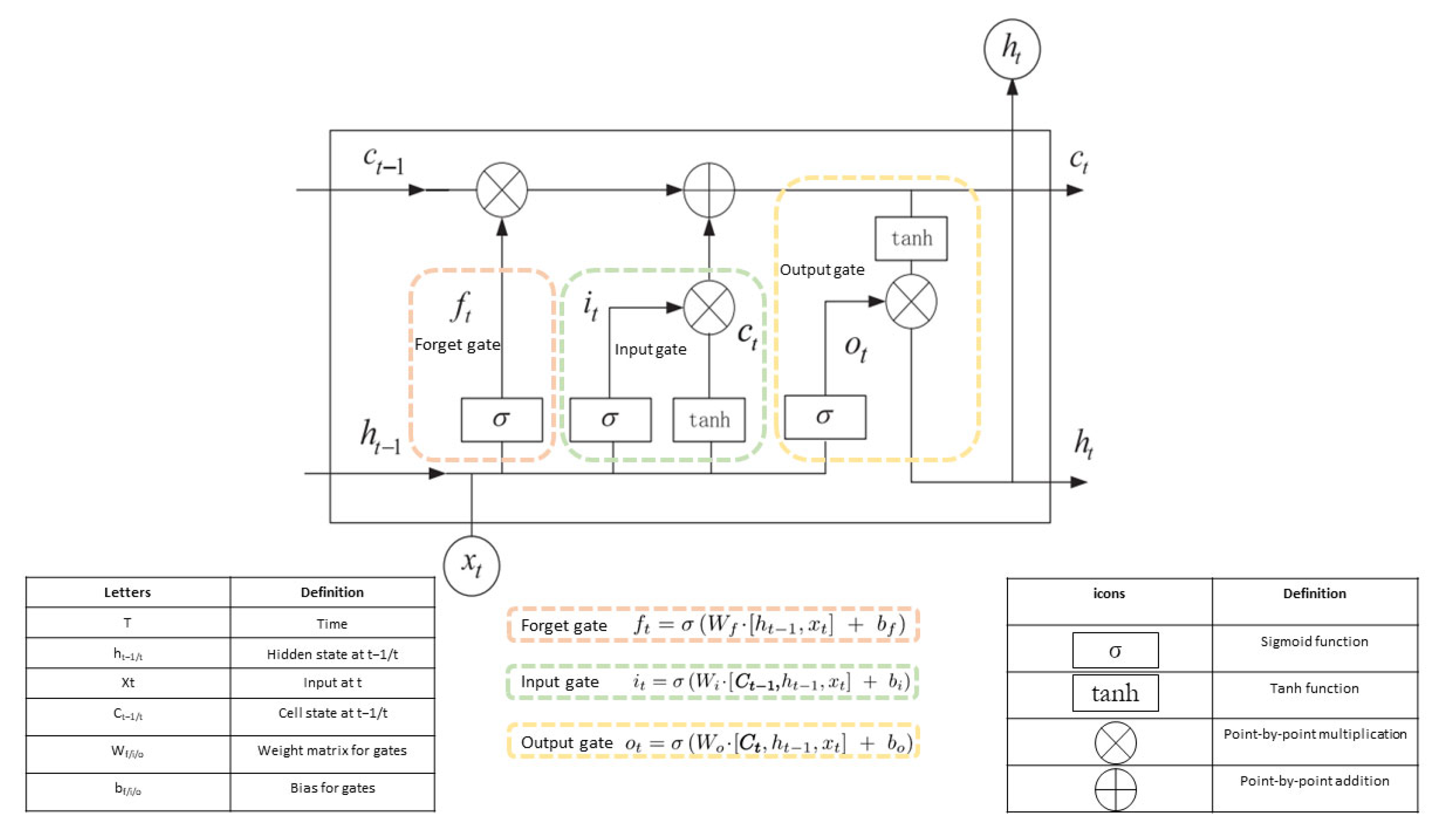
2.3.2. LSTM
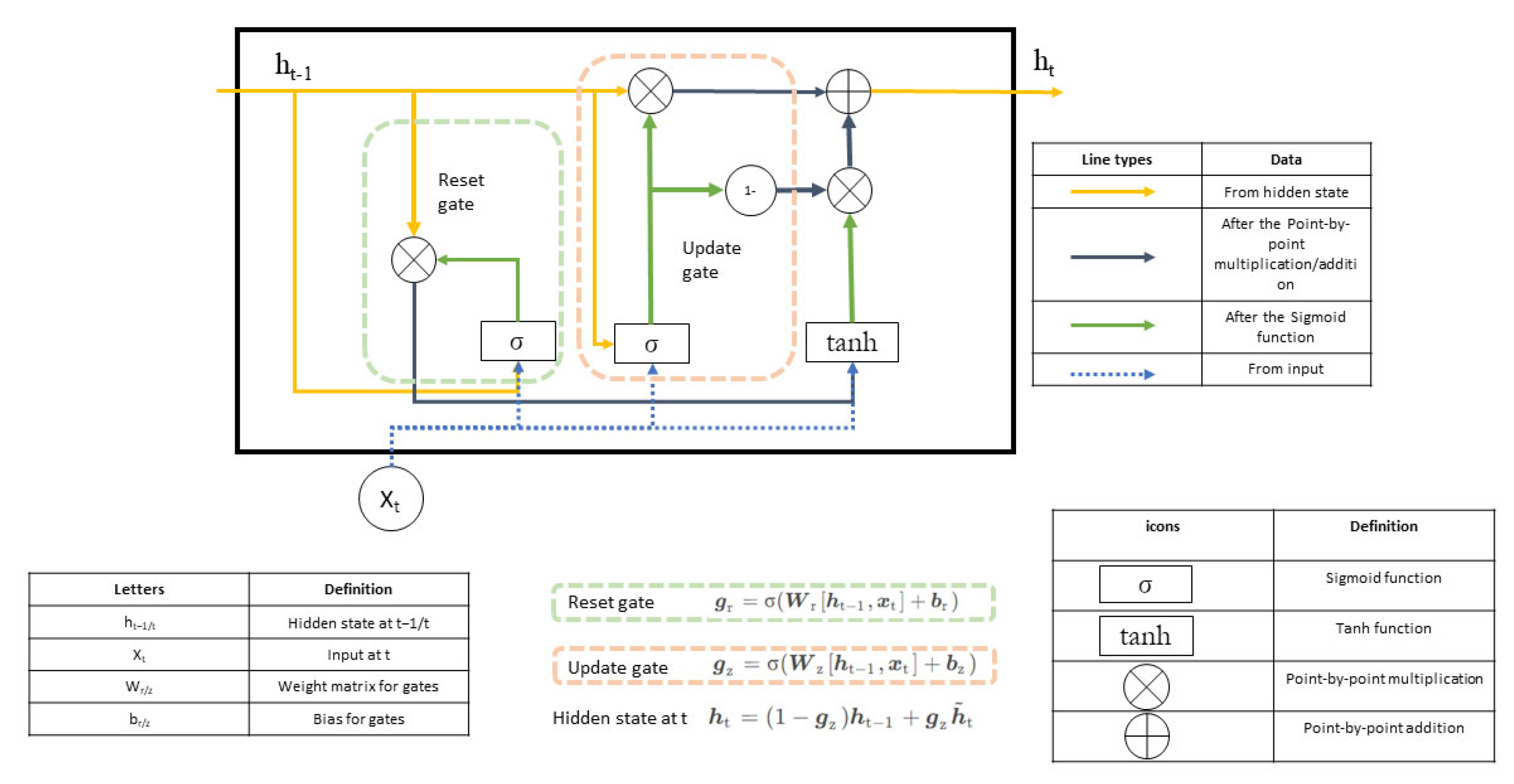
2.3.3. GRU
2.3.4. CNN
2.4. Evaluation Indicators
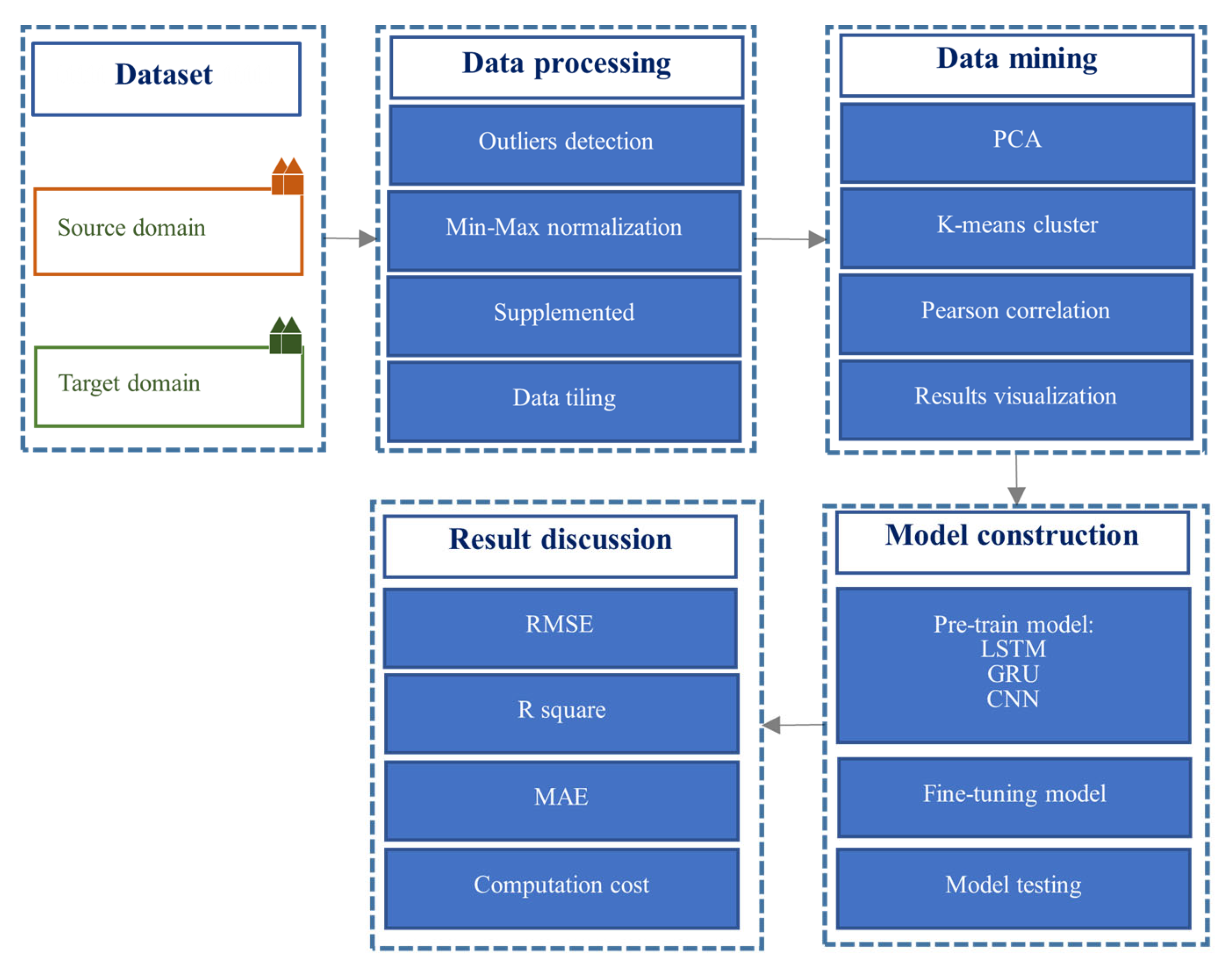
3. Methodology
3.1. Proposed Model
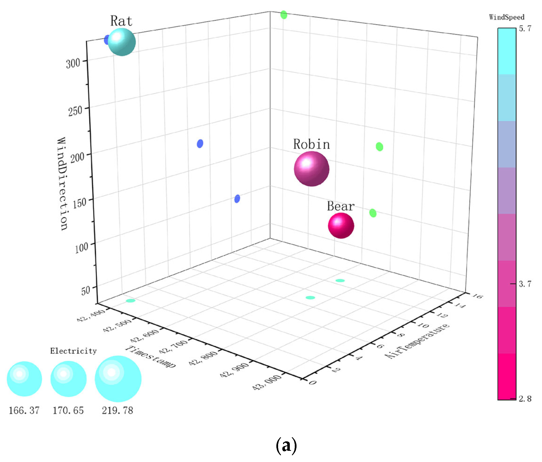
3.2. Dataset
3.3. Data Process
3.4. Data Mining
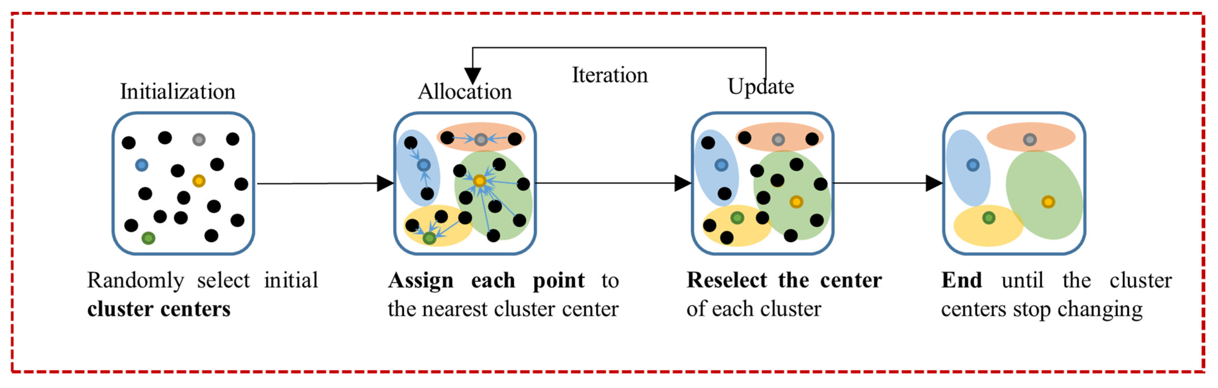
3.4.1. Component Analysis
3.4.2. Calculate Euclidean Distance
3.4.3. Calculate Pearson Coefficient
3.4.4. Combining Euclidean Distance and Pearson Coefficient
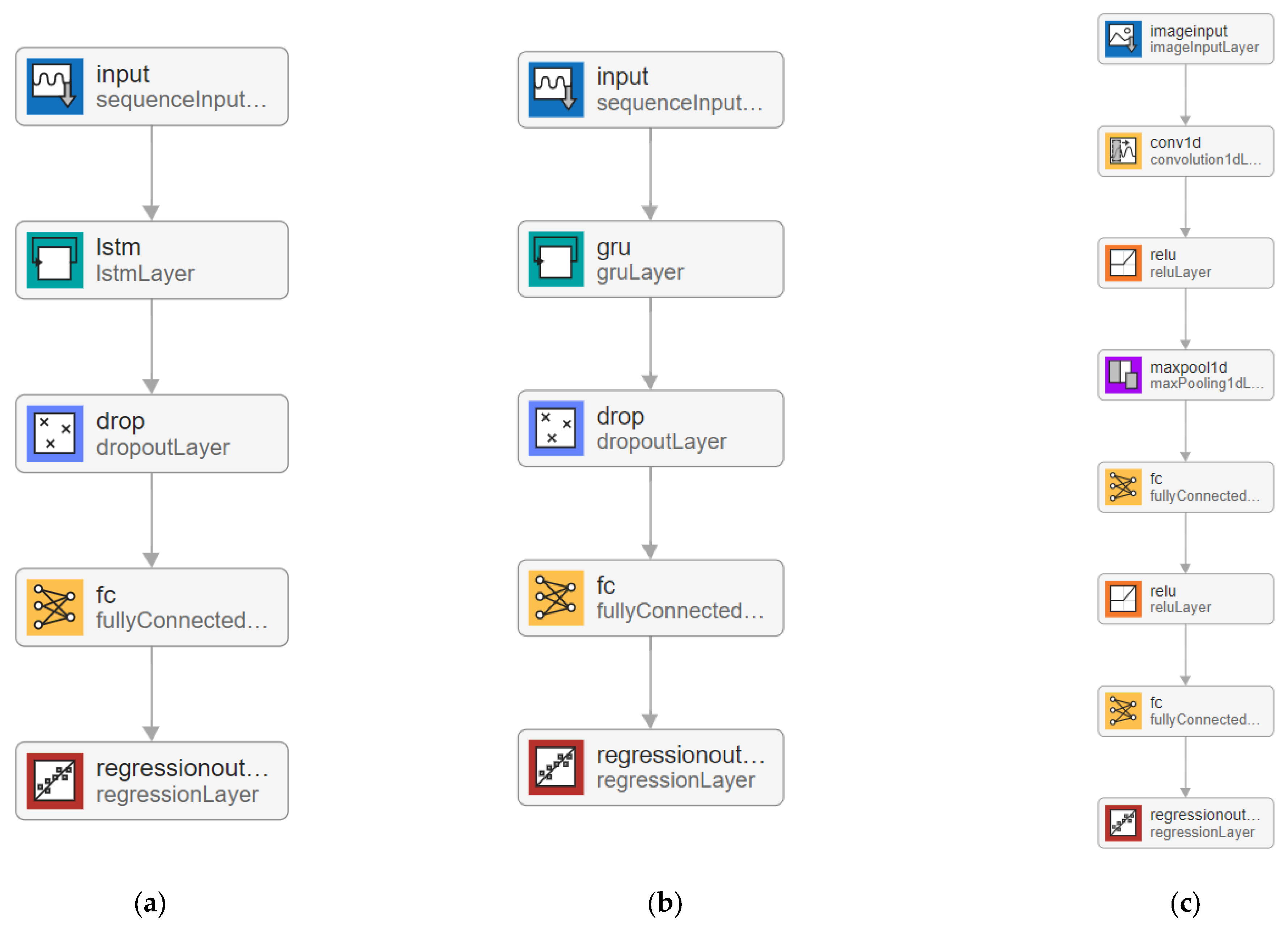
3.5. Data-Driven Model Construction
3.5.1. LSTM
3.5.2. GRU
3.5.3. CNN
3.5.4. Evaluation Indicators
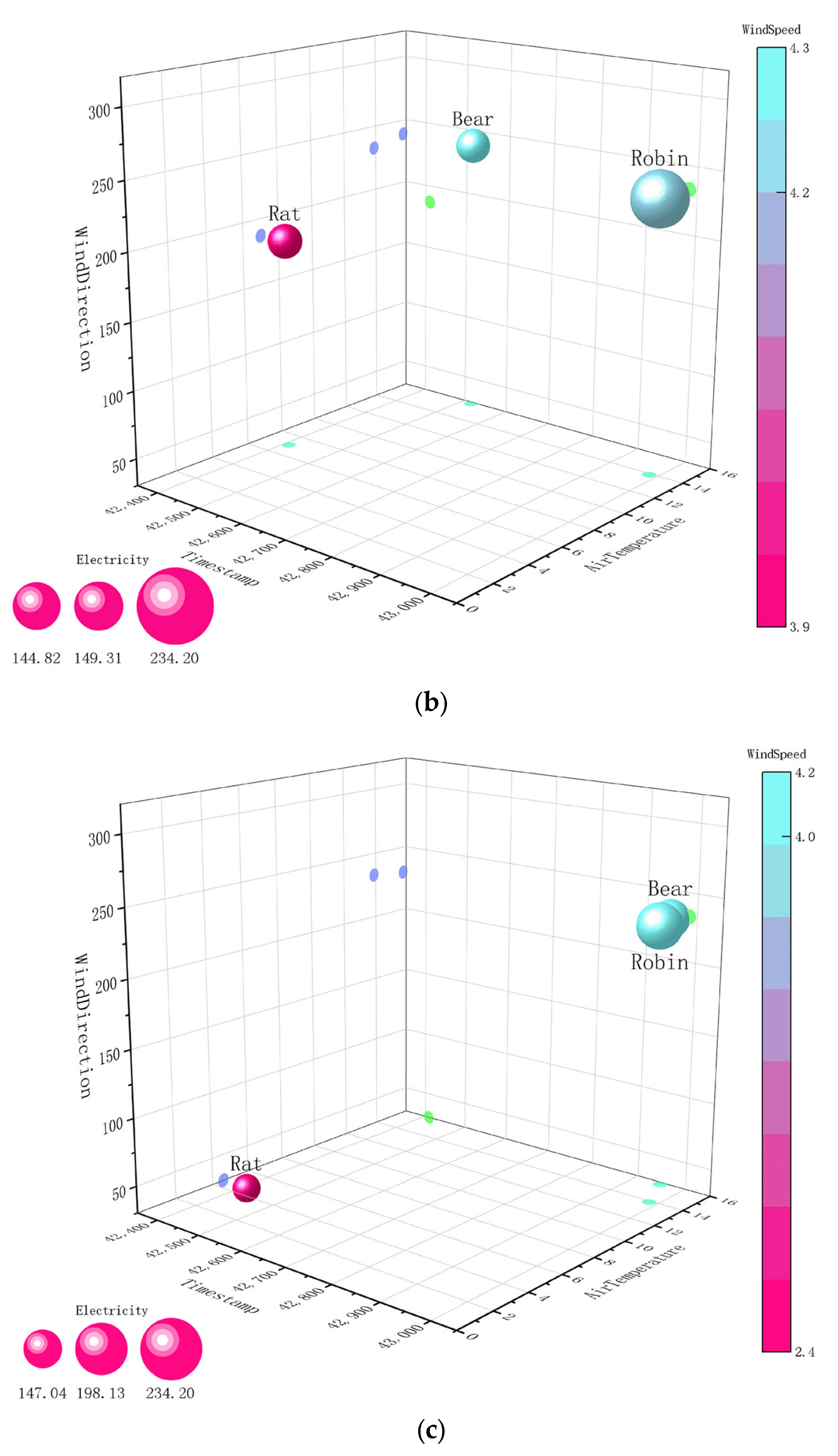
4. Results
4.1. Euclidean Distance and Pearson Correlation
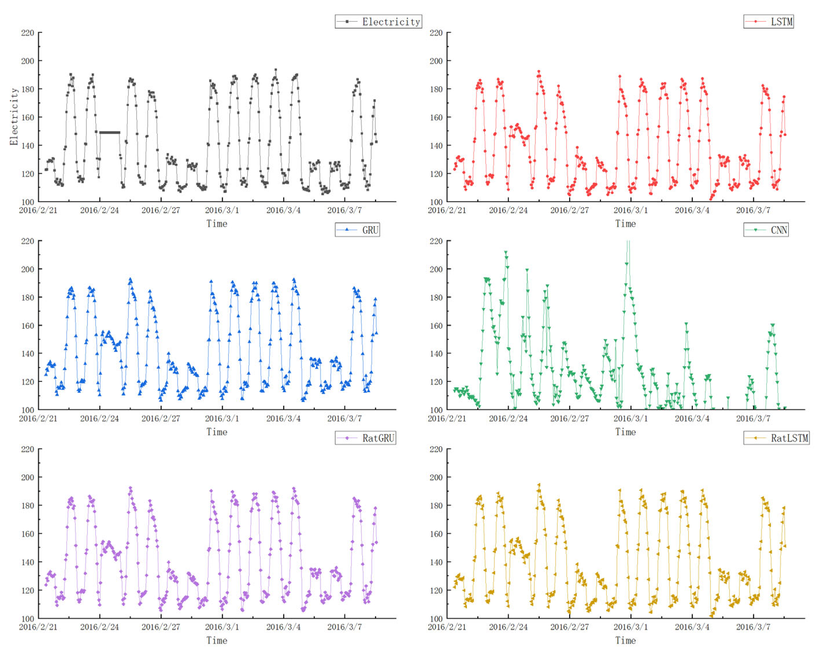
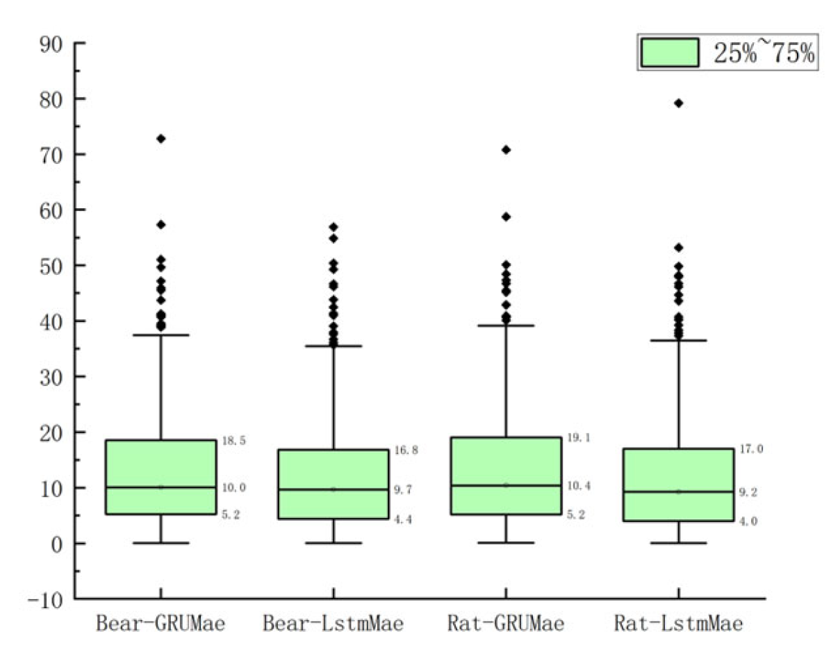
4.2. Transfer Learning Results
4.3. Negative Transfer
5. Discussion
5.1. Key Findings
5.2. Limitation
6. Conclusions
Author Contributions
Funding
Data Availability Statement
Acknowledgments
Conflicts of Interest
Abbreviations
| TL | Transfer Learning |
| LSTM | Long Short-Term Memory |
| GRU | Gated Recurrent Unit |
| CNN | Convolutional Neural Network |
| COP28 | United Nations Climate Change Conference 28 |
| AI | Artificial Intelligence |
| SVM | Support Vector Machine |
| DS | source domain |
| TS | source domain task |
| DT | target domain |
| TT | target task |
| RF | Random Forest |
| RMSE | root-mean-square error |
| MAE | Mean Absolute Error |
| R2 | coefficient of determination |
Appendix A

| Reference | Year | Main Algorithms | Input | Output | Accuracy and Key Findings | |
|---|---|---|---|---|---|---|
| [7] | 2021 | LSTM | 1 | LSTM weather data; energy consumption | LSTM weather data can provide more realistic simulations than meteorological stations and EMP files | |
| [8] | 2023 | LSTM and GRU | 8-month heating load | 24 h heating load | RMSE improved by 37.78% | |
| [9] | 2023 | CNN, GRU, LSTM | Time features, 1, solar radiation, and historical data | 1 h electricity load | RMSE value reduced by 13.64–34.55%; an integrated energy consumption prediction model considering spatial | |
| [10] | 2023 | Bidirectional gate, recurrent unit, CNN, and the residual connection | 1-year heating and cooling load | 1 h heating and cooling load | R2—90.74%; CVRMSE—19.24% | |
| [11] | 2020 | RF | Building material information, 1 | Heating and cooling loads | RMSE—6.97 | |
| [12] | 2023 | ANN, LSTM | Occupant characteristics, travel behavior variables, daily load distribution | Cooling, heating and electric load for different buildings considering EV charging load | R2—0.987 | |
| [13] | 2023 | LSTM, XGB | Cooling loads, meteorological data, and contextual information | Cooling loads of five building types | R2—35.68%, 25.36%, 32.44%, 73.91%, and 37.06%, | |
| [14] | 2023 | LightGBM, RF, and LSTM | 1, electric equipment power density, building material information | Building thermal load | CVRMSE, R2, and computation time are 22.06%, 0.9267, and 758.8 s | |
| [15] | 2023 | ANN, SVR, RF, XGB, LSTM model, hybrid CNN-LSTM model | History electricity load | Daily electricity load | For a building with a low dispersion level, the simple persistence model has satisfactory performance | |
| [16] | 2023 | LSTM, GRU | 24, 12, 6, and 2 h cooling and heating loads | 1 h and 1-day cooling and heating load forecasting of building district energy system | CV-RMSE—14.51% and 11.95% for the 1 h-ahead forecasting of cooling and heating loads | |
| [17] | 2023 | CNN, GRU, LSTM | Electricity demand | 5 min electricity load | RMSE—0.0212 | |
| [18] | 2023 | CNN, LSTM, SVM | Electricity consumption | 1-day electricity consumption | Relative error values—5.26 | Combines the CNN with LSTM to improve performance when weather information is lost |
| [19] | 2023 | SVR, LSTM | Building cooling demands, 1 | Building cooling demands | RMSE—4.33; MAPE—0.66 | |
| [20] | 2023 | CNN | Plug and light load, HVAC electric load, 1, timestamp | Building energy load | MAPE reduced by 7.52%, 4.96%, 6.59%, and 2.34% | An accuracy transfer model based on 1D-CNN |
| [21] | 2023 | BiLSTM, CNN | 1 h electricity consumption | 1-day and 2-day electricity consumption | MAE—9.20 × 10⁻⁴ (1-day) and 9.33 × 10⁻⁴ (2-day) | |
| [22] | 2023 | RF | 1, building cold load | 1-day building cold load | RMSE—7.84 | |
| [23] | 2022 | LSTM, GRU, BILSTM, BIGRU | Outdoor temperature, relative humidity, and load | 15 min building thermal load | MAPE—0.2% | |
| [24] | 2022 | CNN, LSTM, BILSTM | Cooling loads and heating loads | Cooling loads and heating loads | RMSE—0.00874 | |
| [25] | 2022 | CNN, ANN, RF, support vector regression, and gradient boosting tree | Building information | Cooling and heating loads | R2—0.92 | |
| [26] | 2022 | ANN, SVM, ELM, RVM, MLR, RF, and BLR | Whole building’s electric energy consumption; hourly from September 1989 to February 1990 | Whole building’s electric energy consumption | MAPE—1.06 | |
| [27] | 2022 | RF | 1, personnel flow, historical load | Monthly cooling load | RMSE—2.8735 | |
| [28] | 2022 | RF, light GBM | 1, hourly electricity consumption data for five years | Electricity consumption | CVRMSE—12.91 | |
| [29] | 2022 | GRU | Thermal load | Thermal load | Predict thermal load accurately when the meteorological parameters are missing; RMSE—14.63% | |
| [30] | 2022 | GRU, RNN, CNN | Electricity load | Electricity load | RMSE—17.282 | |
| [31] | 2021 | RNN, LSTM | Cooling electricity data | Short-term (1 hour ahead) and long-term (1 day ahead) cooling load | RMSE—37.45; R2—0.9431 | |
| [32] | 2021 | LSTM | Short-term heating load, building information | Short-term heating load | CVRMSE—18.53 | |
| [33] | 2021 | LSTM, RNN, CNN | 1, cooling load | Cooling load | CVRMSE—11.5 | |
| [34] | 2021 | LSTM, SVM, multilayer perceptron | Electric load | Day-ahead electric load | RMSE—10.66 | |
| [35] | 2021 | LSTM, RNN, RF | Electricity load | Short-term electricity load | MAE—4.80 | |
| [36] | 2021 | ANN, SVM, RF | 1, short-term heating load | Short-term heating load | R2—0.90 | |
| [37] | 2021 | ANN, RF, and SVM | 1, building cooling load | Building cooling load | MAE—9.83 | |
| [38] | 2020 | ANN, SVR, LSTM | 1, heating, cooling, lighting loads, and BIPV power production | Heating, cooling, lighting loads, and BIPV power production | MAPE—9.01 | |
| [39] | 2020 | ANN, LSTM, RF, SVM, XGBoost | 1, building information, daily electricity load | Daily electricity load | MAPE—10.69 | |
| [40] | 2020 | LSTM, GRU | Occupant data, plug load, time | Electric loads | RMSE—0.0741 | |
| [41] | 2020 | LSTM, CNN | 1, scheduled related parameters and historical loads | Short-term electrical load forecasting | RMSE—6.24 | |
| [42] | 2020 | RF, SVM, ANN | 1, hourly electricity consumption | Daily electricity load | MAPE—20 | |
References
- United Nations Environment Programme; Global Alliance for Buildings and Construction. 2023 Global Status Report for Buildings and Construction 2024. Available online: https://max.book118.com/html/2024/0704/7003042110006130.shtm (accessed on 14 March 2025).
- Wolf, J. 28 Countries Sign Buildings Breakthrough Agreement at COP28 2023. Available online: https://www.greenbuildingadvisor.com/article/28-countries-sign-buildings-breakthrough-agreement-at-cop28 (accessed on 14 March 2025).
- Ali, D.M.T.E.; Motuzienė, V.; Džiugaitė-Tumėnienė, R. AI-Driven Innovations in Building Energy Management Systems: A Review of Potential Applications and Energy Savings. Energies 2024, 17, 4277. [Google Scholar] [CrossRef]
- Olu-Ajayi, R.; Alaka, H. Building Energy Consumption Prediction Using Deep Learning. J. Build. Eng. 2022, 45, 103406. [Google Scholar] [CrossRef]
- Sun, Y.; Haghighat, F.; Fung, B.C.M. A Review of The-State-of-the-Art in Data-Driven Approaches for Building Energy Prediction. Energy Build. 2020, 221, 110022. [Google Scholar] [CrossRef]
- Janssen, M.; Van Der Voort, H.; Wahyudi, A. Factors Influencing Big Data Decision-Making Quality. J. Bus. Res. 2017, 70, 338–345. [Google Scholar] [CrossRef]
- Zhang, M.; Zhang, X.; Guo, S.; Xu, X.; Chen, J.; Wang, W. Urban micro-climate prediction through long short-term memory network with long-term monitoring for on-site building energy estimation. Sustain. Cities Soc. 2021, 74, 103227. [Google Scholar] [CrossRef]
- Zhou, Y.; Li, X.; Liu, Y.; Wei, R. Transfer learning-based adaptive recursive neural network for short-term non-stationary building heating load prediction. J. Build. Eng. 2023, 76, 107271. [Google Scholar] [CrossRef]
- Cao, W.; Yu, J.; Chao, M.; Wang, J.; Yang, S.; Zhou, M.; Wang, M. Short-term energy consumption prediction method for educational buildings based on model integration. Energy 2023, 283, 128580. [Google Scholar] [CrossRef]
- Wang, L.; Xie, D.; Zhou, L.; Zhang, Z. Application of the hybrid neural network model for energy consumption prediction of office buildings. J. Build. Eng. 2023, 72, 106503. [Google Scholar] [CrossRef]
- Seyedzadeh, S.; Rahimian, F.P.; Oliver, S.; Glesk, I.; Kumar, B. Data driven model improved by multi-objective optimisation for prediction of building energy loads. Autom. Constr. 2020, 116, 103188. [Google Scholar] [CrossRef]
- Zhang, X.; Kong, X.; Yan, R.; Liu, Y.; Xia, P.; Sun, X.; Zeng, R.; Li, H. Data-driven cooling, heating and electrical load prediction for building integrated with electric vehicles considering occupant travel behavior. Energy 2023, 264, 126274. [Google Scholar] [CrossRef]
- Lu, C.; Gu, J.; Lu, W. An improved attention-based deep learning approach for robust cooling load prediction: Public building cases under diverse occupancy schedules. Sustain. Cities Soc. 2023, 96, 104679. [Google Scholar] [CrossRef]
- Chen, Y.; Ye, Y.; Liu, J.; Zhang, L.; Li, W.; Mohtaram, S. Machine Learning Approach to Predict Building Thermal Load Considering Feature Variable Dimensions: An Office Building Case Study. Buildings 2023, 13, 312. [Google Scholar] [CrossRef]
- Hu, M.; Stephen, B.; Browell, J.; Haben, S.; Wallom, D.C.H. Impacts of building load dispersion level on its load forecasting accuracy: Data or algorithms? Importance of reliability and interpretability in machine learning. Energy Build. 2023, 285, 112896. [Google Scholar] [CrossRef]
- Yu, H.; Zhong, F.; Du, Y.; Xie, X.E.; Wang, Y.; Zhang, X.; Huang, S. Short-term cooling and heating loads forecasting of building district energy system based on data-driven models. Energy Build. 2023, 298, 113513. [Google Scholar] [CrossRef]
- Chiu, M.-C.; Hsu, H.-W.; Chen, K.-S.; Wen, C.-Y. A hybrid CNN-GRU based probabilistic model for load forecasting from individual household to commercial building. Energy Rep. 2023, 9, 94–105. [Google Scholar] [CrossRef]
- Chen, P.; Chen, L. Prediction method of intelligent building electricity consumption based on deep learning. Evol. Intell. 2023, 16, 1637–1644. [Google Scholar] [CrossRef]
- Liu, H.; Yu, J.; Dai, J.; Zhao, A.; Wang, M.; Zhou, M. Hybrid prediction model for cold load in large public buildings based on mean residual feedback and improved SVR. Energy Build. 2023, 294, 113229. [Google Scholar] [CrossRef]
- Zhang, Y.; Zhou, Z.; Du, Y.; Shen, J.; Li, Z.; Yuan, J. A data transfer method based on one dimensional convolutional neural network for cross-building load prediction. Energy 2023, 277, 127645. [Google Scholar] [CrossRef]
- Sekhar, C.; Dahiya, R. Robust framework based on hybrid deep learning approach for short term load forecasting of building electricity demand. Energy 2023, 268, 126660. [Google Scholar] [CrossRef]
- Zou, Q.; Wang, L.; Xue, H.; Feng, X.; Qiao, B.; Dong, Y. Random Forest Algorithm Based Dynamictraining Set for Cold Load Prediction. In Proceedings of the 2023 8th Asia Conference on Power and Electrical Engineering (ACPEE), Tianjin, China, 14–16 April 2023; pp. 165–172. [Google Scholar]
- Lv, R.; Yuan, Z.; Lei, B.; Zheng, J.; Luo, X. Building thermal load prediction using deep learning method considering time-shifting correlation in feature variables. J. Build. Eng. 2022, 61, 105316. [Google Scholar] [CrossRef]
- Kavitha, R.J.; Thiagarajan, C.; Priya, P.I.; Anand, A.V.; Al-Ammar, E.A.; Santhamoorthy, M.; Chandramohan, P. Improved Harris Hawks Optimization with Hybrid Deep Learning Based Heating and Cooling Load Prediction on residential buildings. Chemosphere 2022, 309, 136525. [Google Scholar] [CrossRef] [PubMed]
- Lu, J.; Zhang, C.; Li, J.; Zhao, Y.; Qiu, W.; Li, T.; Zhou, K.; He, J. Graph convolutional networks-based method for estimating design loads of complex buildings in the preliminary design stage. Appl. Energy 2022, 322, 119478. [Google Scholar] [CrossRef]
- Li, K.; Zhang, J.; Chen, X.; Xue, W. Building’s hourly electrical load prediction based on data clustering and ensemble learning strategy. Energy Build. 2022, 261, 111943. [Google Scholar] [CrossRef]
- Gao, Z.; Yu, J.; Zhao, A.; Hu, Q.; Yang, S. A hybrid method of cooling load forecasting for large commercial building based on extreme learning machine. Energy 2022, 238, 122073. [Google Scholar] [CrossRef]
- Moon, J.; Rho, S.; Baik, S.W. Toward explainable electrical load forecasting of buildings: A comparative study of tree-based ensemble methods with Shapley values. Sustain. Energy Technol. Assess. 2022, 54, 102888. [Google Scholar] [CrossRef]
- Ma, Z.; Wang, J.; Dong, F.; Wang, R.; Deng, H.; Feng, Y. A decomposition-ensemble prediction method of building thermal load with enhanced electrical load information. J. Build. Eng. 2022, 61, 105330. [Google Scholar] [CrossRef]
- Liu, R.; Chen, T.; Sun, G.; Muyeen, S.M.; Lin, S.; Mi, Y. Short-term probabilistic building load forecasting based on feature integrated artificial intelligent approach. Electr. Power Syst. Res. 2022, 206, 107802. [Google Scholar] [CrossRef]
- Chalapathy, R.; Khoa, N.L.D.; Sethuvenkatraman, S. Comparing multi-step ahead building cooling load prediction using shallow machine learning and deep learning models. Sustain. Energy Grids Netw. 2021, 28, 100543. [Google Scholar] [CrossRef]
- Lu, Y.; Tian, Z.; Zhang, Q.; Zhou, R.; Chu, C. Data augmentation strategy for short-term heating load prediction model of residential building. Energy 2021, 235, 121328. [Google Scholar] [CrossRef]
- Sha, H.; Moujahed, M.; Qi, D. Machine learning-based cooling load prediction and optimal control for mechanical ventilative cooling in high-rise buildings. Energy Build. 2021, 242, 110980. [Google Scholar] [CrossRef]
- Jeong, D.; Park, C.; Ko, Y.M. Short-term electric load forecasting for buildings using logistic mixture vector autoregressive model with curve registration. Appl. Energy 2021, 282, 116249. [Google Scholar] [CrossRef]
- Bellahsen, A.; Dagdougui, H. Aggregated short-term load forecasting for heterogeneous buildings using machine learning with peak estimation. Energy Build. 2021, 237, 110742. [Google Scholar] [CrossRef]
- Zhou, Y.; Liu, Y.; Wang, D.; Liu, X. Comparison of machine-learning models for predicting short-term building heating load using operational parameters. Energy Build. 2021, 253, 111505. [Google Scholar] [CrossRef]
- Zhang, C.; Li, J.; Zhao, Y.; Li, T.; Chen, Q.; Zhang, X.; Qiu, W. Problem of data imbalance in building energy load prediction: Concept, influence, and solution. Appl. Energy 2021, 297, 117139. [Google Scholar] [CrossRef]
- Luo, X.J.; Oyedele, L.O.; Ajayi, A.O.; Akinade, O.O. Comparative study of machine learning-based multi-objective prediction framework for multiple building energy loads. Sustain. Cities Soc. 2020, 61, 102283. [Google Scholar] [CrossRef]
- Cao, L.; Li, Y.; Zhang, J.; Jiang, Y.; Han, Y.; Wei, J. Electrical load prediction of healthcare buildings through single and ensemble learning. Energy Rep. 2020, 6, 2751–2767. [Google Scholar] [CrossRef]
- Das, A.; Annaqeeb, M.K.; Azar, E.; Novakovic, V.; Kjærgaard, M.B. Occupant-centric miscellaneous electric loads prediction in buildings using state-of-the-art deep learning methods. Appl. Energy 2020, 269, 115135. [Google Scholar] [CrossRef]
- Chitalia, G.; Pipattanasomporn, M.; Garg, V.; Rahman, S. Robust short-term electrical load forecasting framework for commercial buildings using deep recurrent neural networks. Appl. Energy 2020, 278, 115410. [Google Scholar] [CrossRef]
- Walker, S.; Khan, W.; Katic, K.; Maassen, W.; Zeiler, W. Accuracy of different machine learning algorithms and added-value of predicting aggregated-level energy performance of commercial buildings. Energy Build. 2020, 209, 109705. [Google Scholar] [CrossRef]
- Yuan, Y.; Chen, Z.; Wang, Z.; Sun, Y.; Chen, Y. Attention mechanism-based transfer learning model for day-ahead energy demand forecasting of shopping mall buildings. Energy 2023, 270, 126878. [Google Scholar] [CrossRef]
- Wang, Z.; Hong, T.; Piette, M.A. Building thermal load prediction through shallow machine learning and deep learning. Appl. Energy 2020, 263, 114683. [Google Scholar] [CrossRef]
- Jebli, I.; Belouadha, F.-Z.; Kabbaj, M.I.; Tilioua, A. Prediction of Solar Energy Guided by Pearson Correlation Using Machine Learning. Energy 2021, 224, 120109. [Google Scholar] [CrossRef]
- Jung, S.-M.; Park, S.; Jung, S.-W.; Hwang, E. Monthly Electric Load Forecasting Using Transfer Learning for Smart Cities. Sustainability 2020, 12, 6364. [Google Scholar] [CrossRef]
- Peng, C.; Tao, Y.; Chen, Z.; Zhang, Y.; Sun, X. Multi-source transfer learning guided ensemble LSTM for building multi-load forecasting. Expert Syst. Appl. 2022, 202. [Google Scholar] [CrossRef]
- Iglesias, F.; Kastner, W. Analysis of Similarity Measures in Times Series Clustering for the Discovery of Building Energy Patterns. Energies 2013, 6, 579–597. [Google Scholar] [CrossRef]
- Bozinovski, S. Reminder of the first paper on transfer learning in neural networks, 1976. Informatica 2020, 44. [Google Scholar] [CrossRef]
- Wu, X.; Khorshidi, H.A.; Aickelin, U.; Edib, Z.; Peate, M. Transfer Learning to Enhance Amenorrhea Status Prediction in Cancer and Fertility Data with Missing Values. In Artificial Intelligence; Productivity Press: New York, NY, USA, 2020; pp. 233–260. ISBN 978-0-429-31741-5. [Google Scholar]
- Pan, S.J.; Yang, Q. A Survey on Transfer Learning. IEEE Trans. Knowl. Data Eng. 2010, 22, 1345–1359. [Google Scholar] [CrossRef]
- Weiss, K.; Khoshgoftaar, T.M.; Wang, D. A survey of transfer learning. J. Big Data 2016, 3, 1345–1459. [Google Scholar] [CrossRef]
- Wu, Q.; Wu, H.; Zhou, X.; Tan, M.; Xu, Y.; Yan, Y.; Hao, T. Online Transfer Learning with Multiple Homogeneous or Heterogeneous Sources. IEEE Trans. Knowl. Data Eng. 2017, 29, 1494–1507. [Google Scholar] [CrossRef]
- Santosh, T.; Ichim, O.; Grabmair, M. Zero-shot transfer of article-aware legal outcome classification for European Court of human rights cases. arXiv 2023, arXiv:2302.00609. [Google Scholar]
- Gao, Y.; Ruan, Y.; Fang, C.; Yin, S. Deep learning and transfer learning models of energy consumption forecasting for a building with poor information data. Energy Build. 2020, 223, 110156. [Google Scholar] [CrossRef]
- Zhang, L.; Wen, J.; Li, Y.; Chen, J.; Ye, Y.; Fu, Y.; Livingood, W. A review of machine learning in building load prediction. Appl. Energy 2021, 285, 116452. [Google Scholar] [CrossRef]
- Ali, S.; Abuhmed, T.; El-Sappagh, S.; Muhammad, K.; Alonso-Moral, J.M.; Confalonieri, R.; Guidotti, R.; Del Ser, J.; Díaz-Rodríguez, N.; Herrera, F. Explainable Artificial Intelligence (XAI): What we know and what is left to attain Trustworthy Artificial Intelligence. Inf. Fusion 2023, 99, 101805. [Google Scholar] [CrossRef]
- Li, L.; Su, X.; Bi, X.; Lu, Y.; Sun, X. A novel Transformer-based network forecasting method for building cooling loads. Energy Build. 2023, 296, 113409. [Google Scholar] [CrossRef]
- Thilker, C.A.; Bacher, P.; Bergsteinsson, H.G.; Junker, R.G.; Cali, D.; Madsen, H. Non-linear grey-box modelling for heat dynamics of buildings. Energy Build. 2021, 252, 111457. [Google Scholar] [CrossRef]
- Harb, H.; Boyanov, N.; Hernandez, L.; Streblow, R.; Müller, D. Development and validation of grey-box models for forecasting the thermal response of occupied buildings. Energy Build. 2016, 117, 199–207. [Google Scholar] [CrossRef]
- Cho, K. Learning phrase representations using RNN encoder-decoder for statistical machine translation. arXiv 2014, arXiv:1406.1078. [Google Scholar]
- Kiranyaz, S.; Avci, O.; Abdeljaber, O.; Ince, T.; Gabbouj, M.; Inman, D.J. 1D convolutional neural networks and applications: A survey. Mech. Syst. Signal Process. 2021, 151, 107398. [Google Scholar] [CrossRef]
| Feature Extraction | Fine-Tuning | |
|---|---|---|
| Definition | Keeping the feature extraction layer of the pre-trained model unchanged and only training the newly added output layer. This approach leverages the generic features learned by the pre-trained model on large-scale datasets while customizing the model through the new output layer. Usually, this involves freezing the weights and extracting useful features. | Using the entire pre-trained model as the initial model and then training the entire model using the new dataset. This means that all parameters of the model, including the weights of the pre-trained model and the new output layer, will be relearned. Usually, this involves freezing the earlier layers. |
| Workflow | 1. Load the pre-trained model. 2. Freeze the feature extraction layer. 3. Add a new output layer. 4. Train only the newly added output layer. | 1. Load the pre-trained model. 2. Modify the output layer to suit the new task. 3. Load the new dataset. 4. Train the entire model. |
| Advantages | Usually requires less data and computing resources. | Enables the model to fully adapt to the data distribution of the new task. |
| Disadvantages | Prone to overfitting. | Requires a significant amount of new data and computational costs. |
| Building_Id | Spaceusage | Sqm | Location | Electricity |
|---|---|---|---|---|
| Rat_education_Lynn | Education-K-12 School | 7785.3 | US/Eastern | 29–260 |
| Bear_education_Pattie | Education | 8032.9 | US/Pacific | 92–329 |
| Robin_education_Zenia (Target) | Education-College Laboratory | 6337.0 | Europe/London | 52–466 |
| timestamp | airTemperature | seaLvlPressure | windDirection | windSpeed | Electricity |
|---|---|---|---|---|---|
| Serial value | °C | kPa | ° | m/s | kWh |
| Component | |||
|---|---|---|---|
| 1 | 2 | 3 | |
| timestamp | 0.200 | −0.101 | 0.949 |
| airTemperature | 0.916 | 0.148 | 0.010 |
| Dewtemperature | 0.962 | 0.034 | −0.023 |
| seaLvlPressure | −0.439 | −0.596 | 0.204 |
| windDirection | −0.306 | 0.719 | 0.233 |
| windSpeed | −0.241 | 0.789 | 0.063 |
| Slover | Learning Rate Initial | Batch Size | Epoch | Momentum |
|---|---|---|---|---|
| Adam | 1 × 10⁻³ | 128 | 30 | 0.9 |
| LearnRateSchedule | LearnRateDropFactor | LearnRateDropPeriod | Hidden Unit | |
| piecewise | 0.1 | 400 | 8 | |
| Slover | Learning Rate Initial | Batch Size | Epoch | Verbose |
|---|---|---|---|---|
| Adam | 1 × 10⁻³ | 128 | 30 | False |
| LearnRateSchedule | LearnRateDropFactor | LearnRateDropPeriod | Hidden Unit | |
| piecewise | 0.1 | 400 | 32 | |
| Slover | Learning Rate Initial | Batch Size |
|---|---|---|
| Adam | 0.005 | 128 |
| Epoch | Verbose | Kernel |
| 30 | False | [57] |
| Building | Group | timestamp | airTemperature | seaLvlPressure | windDirection | windSpeed | Electricity |
| Rat_ Edu_ Lynn | 1 | 42,402.25 | 1.6 | 1018.7 | 318 | 5.7 | 166.37 |
| 2 | 42,409.84 | 7 | 1016.7 | 187 | 3.9 | 144.82 | |
| 3 | 42,408.71 | 4.6 | 1019.8 | 30 | 2.4 | 147.04 | |
| Building | Group | timestamp | airTemperature | seaLvlPressure | windDirection | windSpeed | Electricity |
| Bear_ Edu_ Pattie | 1 | 42,735.66 | 12.6 | 1017.4 | 97 | 2.8 | 170.6491 |
| 2 | 42,520.93 | 15.8 | 1016.6 | 239 | 4.3 | 149.309 | |
| 3 | 42,952.07 | 15.8 | 1016.3 | 230 | 4 | 198.1281 | |
| Building | Group | timestamp | airTemperature | seaLvlPressure | windDirection | windSpeed | Electricity |
| Rob_ Edu_ Zenia | 1 | 42,752.38 | 9.1 | 1019.4 | 179 | 3.7 | 219.7798 |
| 2 | 42,502.41 | 12.5 | 1014.1 | 204 | 4.2 | 155.1575 | |
| 3 | 42,984.45 | 13.9 | 1015.3 | 233 | 4.2 | 234.195 |
| Robin-timestamp | Robin-airTemperature | Robin-seaLvlPressure | Robin-windDirection | Robin-windSpeed | ||
|---|---|---|---|---|---|---|
| Robin_education_Zenia | Pearson correlation | 0.600 ** | 0.329 ** | 0.085 ** | 0.035 ** | 0.072 ** |
| Sig. (2-tailed) | <0.001 | <0.001 | <0.001 | <0.001 | <0.001 | |
| N | 17,544 | 17,544 | 17,544 | 17,544 | 17,544 | |
| Robin-timestamp | Robin-airTemperature | Robin-timestamp | Robin-airTemperature | ||||
|---|---|---|---|---|---|---|---|
| Rat-airTemperature | Pearson correlation | 0.113 ** | 0.754 ** | Bear-airTemperature | Pearson correlation | 0.01 | 0.619 ** |
| Sig. (2-tailed) | <0.001 | <0.001 | Sig. (2-tailed) | 0.06 | <0.001 | ||
| Rat-seaLvlPressure | Pearson correlation | 0.039 ** | −0.114 ** | Bear-seaLvlPressure | Pearson correlation | −0.045 ** | −0.346 ** |
| Sig. (2-tailed) | <0.001 | <0.001 | Sig. (2-tailed) | <0.001 | <0.001 | ||
| Rat-windDirection | Pearson correlation | (0.01) | −0.055 ** | Bear-windDirection | Pearson correlation | −0.028 ** | 0.392 ** |
| Sig. (2-tailed) | 0.47 | 0.00 | Sig. (2-tailed) | <0.001 | <0.001 | ||
| Rat-windSpeed | Pearson correlation | −0.060 ** | (0.01) | Bear-windSpeed | Pearson correlation | −0.077 ** | 0.305 ** |
| Sig. (2-tailed) | <0.001 | 0.32 | Sig. (2-tailed) | <0.001 | <0.001 | ||
| Group 1 | Group 2 | Group 3 | |||
|---|---|---|---|---|---|
| Rat | 380.559 | Rat | 583.382 | Rat | 616.758 |
| Bear | 97.131 | Bear | 471.277 | Bear | 48.610 |
| Bear-GRU | Bear-LSTM | Rat-GRU | Rat-LSTM | Bear-CNN | |
|---|---|---|---|---|---|
| RMSE | 6.50 | 6.21 | 6.47 | 6.19 | 33.21 |
| R2 | 0.926 | 0.922 | 0.928 | 0.923 | 0.7 |
| Computation cost(s) | 29 | 24 | 83 | 71 | 8 |
| GRU | LSTM | Base-GRU | Base-LSTM | |
|---|---|---|---|---|
| RMSE | 6.75 | 7.73 | <6.75 | <7.73 |
| R2 | 0.91 | 0.90 | >0.91 | >0.90 |
| Computation cost(s) | 82 | 69 | - | - |
Disclaimer/Publisher’s Note: The statements, opinions and data contained in all publications are solely those of the individual author(s) and contributor(s) and not of MDPI and/or the editor(s). MDPI and/or the editor(s) disclaim responsibility for any injury to people or property resulting from any ideas, methods, instructions or products referred to in the content. |
© 2025 by the authors. Licensee MDPI, Basel, Switzerland. This article is an open access article distributed under the terms and conditions of the Creative Commons Attribution (CC BY) license (https://creativecommons.org/licenses/by/4.0/).
Share and Cite
Luo, C.; Xia, L.; Hong, S.-H. A Method for Selecting the Appropriate Source Domain Buildings for Building Energy Prediction in Transfer Learning: Using the Euclidean Distance and Pearson Coefficient. Energies 2025, 18, 3706. https://doi.org/10.3390/en18143706
Luo C, Xia L, Hong S-H. A Method for Selecting the Appropriate Source Domain Buildings for Building Energy Prediction in Transfer Learning: Using the Euclidean Distance and Pearson Coefficient. Energies. 2025; 18(14):3706. https://doi.org/10.3390/en18143706
Chicago/Turabian StyleLuo, Chuyi, Liang Xia, and Sung-Hugh Hong. 2025. "A Method for Selecting the Appropriate Source Domain Buildings for Building Energy Prediction in Transfer Learning: Using the Euclidean Distance and Pearson Coefficient" Energies 18, no. 14: 3706. https://doi.org/10.3390/en18143706
APA StyleLuo, C., Xia, L., & Hong, S.-H. (2025). A Method for Selecting the Appropriate Source Domain Buildings for Building Energy Prediction in Transfer Learning: Using the Euclidean Distance and Pearson Coefficient. Energies, 18(14), 3706. https://doi.org/10.3390/en18143706