A CNN-SA-GRU Model with Focal Loss for Fault Diagnosis of Wind Turbine Gearboxes

Abstract

Gearbox failures are a major cause of unplanned downtime and increased maintenance costs, making accurate diagnosis crucial in ensuring wind turbine reliability and cost-efficiency. However, most existing diagnostic methods fail to fully extract the spatiotemporal features in SCADA data and neglect the impact of class imbalance, thereby limiting diagnostic accuracy. To address these challenges, this paper proposes a fault diagnosis model for wind turbine gearboxes based on CNN-SA-GRU and Focal Loss. Specifically, a CNN-SA-GRU network is constructed to extract both spatial and temporal features, in which CNN is employed to extract local spatial features from SCADA data, Shuffle Attention is integrated to efficiently fuse channel and spatial information and enhance spatial representation, and GRU is utilized to capture long-term spatiotemporal dependencies. To mitigate the adverse effects of class imbalance, the conventional cross-entropy loss is replaced with Focal Loss, which assigns higher weights to hard-to-classify fault samples. Finally, the model is validated using real wind farm data. The results show that, compared with the cross-entropy loss, using Focal Loss improves the accuracy and F1 score by an average of 0.24% and 1.03%, respectively. Furthermore, the proposed model outperforms other baseline models with average gains of 0.703% in accuracy and 4.65% in F1 score.

1. Introduction

As a green and renewable energy source, wind power has experienced rapid development worldwide. However, due to the harsh environmental conditions and highly variable operating states of wind turbines, their reliability remains relatively low, with a persistently high failure rate. Statistics show that the operation and maintenance (O&M) costs of onshore wind turbines account for approximately 10–15% of the total power generation cost, while for offshore wind turbines, this proportion increases to around 20–25% [1]. The substantial O&M expenses impose a significant burden on wind farm operators. Therefore, there is an urgent need to develop an efficient and accurate fault diagnosis model that can promptly detect failures and identify fault types, thereby reducing downtime and lowering O&M costs.

Currently, fault diagnosis methods for wind turbines can be broadly categorized into two main approaches: model-based methods [2,3,4] and data-driven methods [5,6,7]. Model-based methods establish physical or mathematical models to represent turbine components and monitor their conditions by comparing measured values with theoretical predictions. However, such methods are often difficult to implement, costly, and highly dependent on accurate data and generally lack adaptability across different systems. In contrast, data-driven methods rely on advanced artificial intelligence algorithms and do not require the construction of complex theoretical models, meaning that they are widely applied in wind turbine fault diagnosis. Based on the type of data used, data-driven methods can be further divided into four categories: vibration signals [8,9,10], acoustic emission signals [11], oil analysis signals [12], and SCADA data [13,14,15].

Fault diagnosis methods based on vibration signals typically involve installing vibration sensors to analyze high-frequency signals for fault identification. For instance, Jiang et al. [16] designed a novel multi-scale convolutional neural network (MSCNN) to extract multi-scale features from raw vibration signals, enabling end-to-end intelligent fault diagnosis in wind turbine gearboxes. However, such methods are costly, susceptible to noise interference, challenging in terms of feature extraction, and heavily reliant on expert knowledge, which limits their accuracy and timeliness in practical applications. Acoustic emission technology utilizes high-frequency, non-contact signal acquisition and serves as a high-frequency, non-destructive testing technique. For example, Chen et al. [17] proposed a yaw system acoustic damage detection method based on Bayesian networks, achieving the accurate characterization of the yaw system’s condition and damage detection. Oil analysis methods primarily assess gearbox operating conditions by analyzing the physical and chemical properties of the lubricating oil, such as the viscosity, temperature, and impurity content. For example, Kerman et al. [18] monitored the particle count in the gearbox lubricant using an optical debris sensor and evaluated gearbox health by analyzing the rate of change in particle quantity. Nevertheless, diagnostic methods based on acoustic emission and oil analysis also suffer from poor anti-interference capability, high dependence on expert knowledge, and the need for on-site data acquisition. These limitations result in low efficiency and hinder their applicability in real-world wind turbine operations.

At present, most wind turbines are equipped with SCADA systems to continuously monitor their operational status and performance. SCADA systems typically record large volumes of sensor data at intervals ranging from a few seconds to several minutes. As wind turbines operate over extended periods, these systems accumulate vast amounts of monitoring data without the need for additional sensors or data acquisition devices. Embedded within this data are valuable monitoring and diagnostic insights that reflect the health condition of the wind turbines. Therefore, research on fault diagnosis using SCADA data has received increasing attention in the wind power field.

Liu et al. [19] proposed a condition monitoring model based on spatiotemporal graph neural networks, which constructs a graph structure among multivariate variables using a Top-k nearest neighbor strategy and extracts features from SCADA data by stacking multiple spatiotemporal blocks for prediction. Pang et al. [20] developed a Spatiotemporal Fusion Neural Network (STFNN), which utilizes multi-kernel convolutional neural networks to extract spatial features from multivariate SCADA data and incorporates an LSTM network to model temporal dependencies, enabling end-to-end fault diagnosis for wind turbines. Feng et al. [21] innovatively integrated five types of explicit rule-based knowledge into data-driven implicit knowledge. They employed an attention mechanism to generate a fused adjacency matrix and constructed a prediction model using a multivariate temporal graph neural network, achieving accurate fault localization through explicit–implicit knowledge fusion. Wang et al. [22] proposed an enhanced model, SLFormer, which combines LSTM networks with Transformer encoders for early fault detection in wind turbine gearboxes. Lei et al. [23] introduced a novel fault diagnosis framework based on an end-to-end LSTM model that directly learns features from multivariate time series data, enabling multi-class fault diagnosis for wind turbines.

In summary, the aforementioned studies have achieved promising results in condition monitoring and diagnosis in wind turbines using SCADA data. However, due to the complex dynamic spatiotemporal correlations inherent in SCADA data, several limitations remain in existing fault diagnosis models: (1) These methods exhibit limitations in extracting spatiotemporal features, particularly in capturing localized spatial dependencies. (2) They often fail to adequately address the scarcity of fault samples within SCADA datasets, especially the severe class imbalance among different fault categories. (3) Most approaches focus on single-variable warning analysis, neglecting the strong inter-variable coupling caused by thermal conduction effects within turbine components, which compromises the model’s ability to accurately locate faults. To address these issues, this paper proposes a fault diagnosis model for wind turbine gearboxes based on CNN-SA-GRU and Focal Loss. The main contributions of this work are as follows:

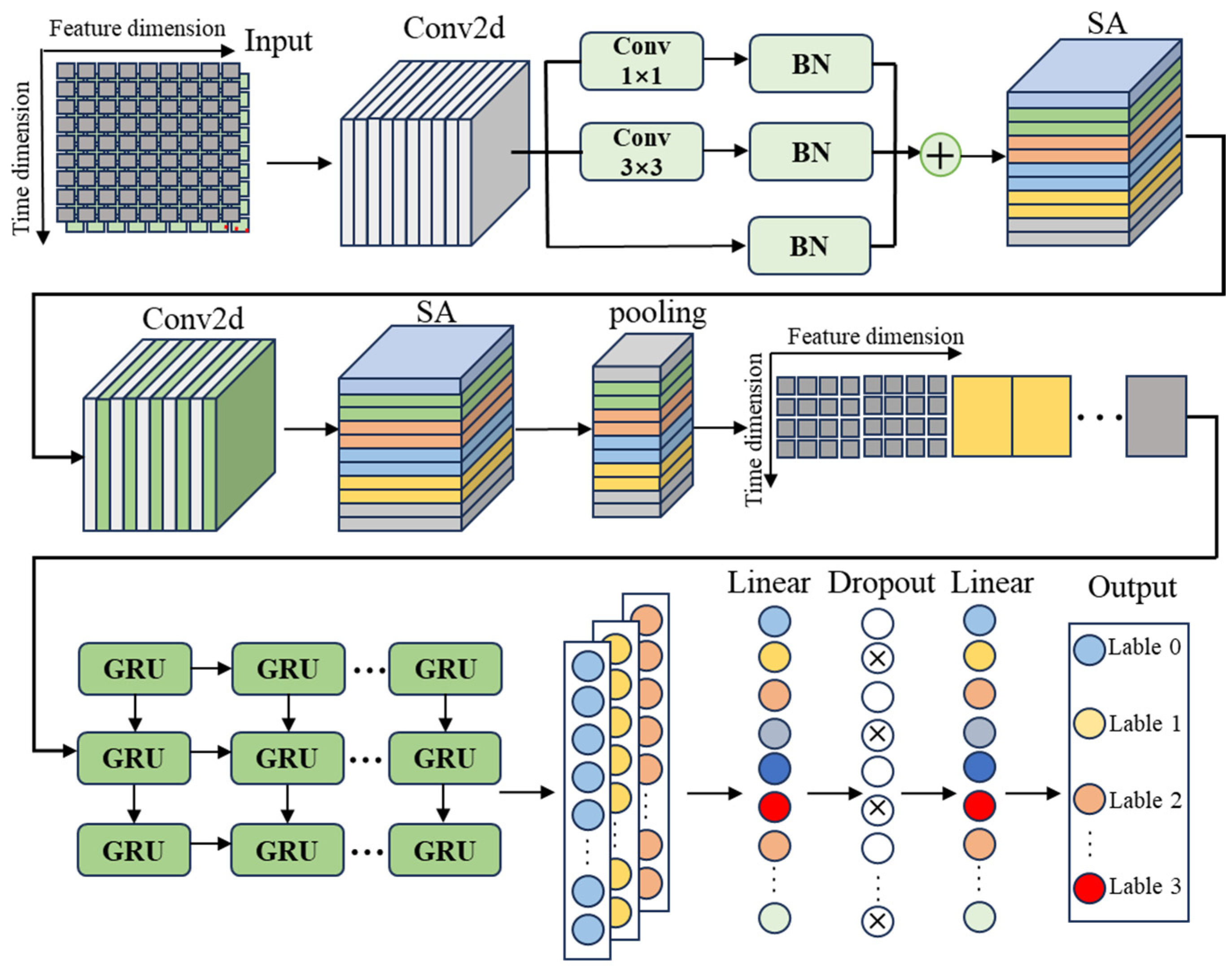
• To capture the spatiotemporal dependencies in SCADA data, a novel CNN-SA-GRU model is proposed. This model enables the deep mining of multi-scale spatiotemporal features embedded in SCADA data, thereby enhancing fault classification accuracy.
• To mitigate the negative impact of fault sample scarcity and class imbalance on diagnostic performance, Focal Loss is employed in place of traditional cross-entropy loss. By assigning higher weights to hard-to-classify samples, the model’s diagnostic capability is significantly improved.

The structure of the remaining parts of this paper is as follows: Section 2 outlines the fault diagnosis process for wind turbine gearboxes. Section 3 presents the structure and working principles of the proposed CNN-SA-GRU model. Section 4 presents a case study using real-world wind farm data. Section 5 concludes the paper.

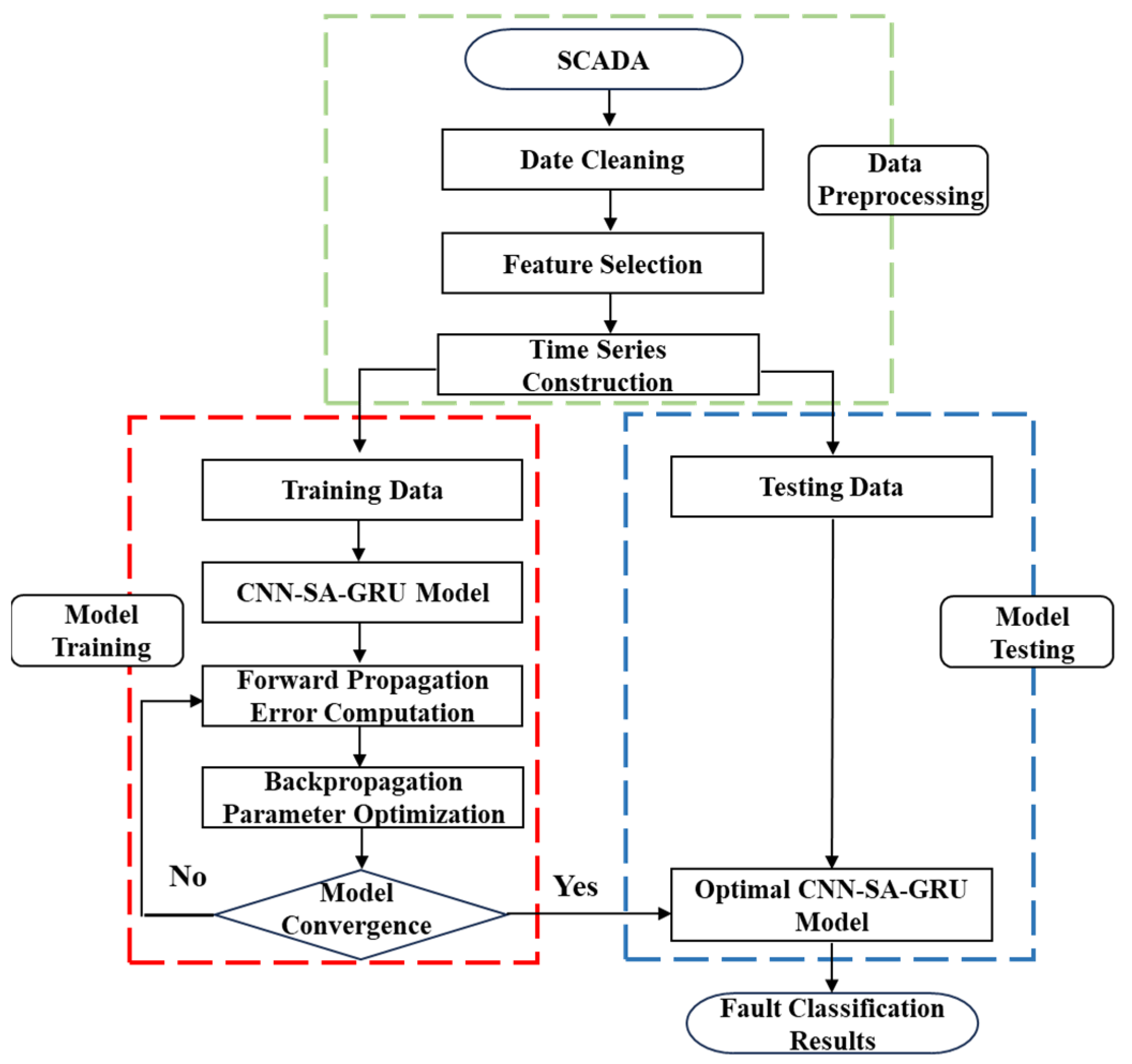
2. Fault Diagnosis Process for Wind Turbine Gearboxes

Figure 1 illustrates the process of fault diagnosis in wind turbine gearboxes. As shown, the proposed method primarily consists of three modules: data preprocessing, offline model training, and online diagnosis. During the data preprocessing stage, data cleaning is first performed to remove invalid or abnormal data caused by factors such as turbine shutdowns due to faults, wind speeds below the cut-in threshold, or wind speeds exceeding the cut-out threshold. Next, Pearson correlation analysis is employed to evaluate the relationships among input variables, and features that exhibit high correlation with the target variable are selected as model inputs. This step helps reduce data redundancy and improve model performance. Subsequently, a sliding window approach is used to segment the continuous SCADA data into two-dimensional temporal subsequences. These are further expanded into three-dimensional input data to meet the training requirements of the subsequent deep learning model. During the offline training stage, a multi-class fault classifier is trained using a large amount of labeled SCADA data collected from wind farms. The classifier is based on the proposed CNN-SA-GRU model and is capable of distinguishing between normal operation and various fault conditions. In the online diagnosis stage, preprocessed samples are directly fed into the trained and optimized CNN-SA-GRU model to obtain fault classification results, i.e., the corresponding fault labels.

2.1. Data Normalization

In this study, the data preprocessing stage includes outlier removal and normalization. During the training process, only SCADA data collected under the normal operating condition of the wind turbine is used. To minimize the impact of differing units across parameters, the input data is normalized using the following equation:

$$x^{\prime }={\displaystyle \frac{x-\min (x)}{\max (x)-\min (x)}}$$

(1)

where x’ is the normalized value of the raw data x, and max(x) and min(x) denote the maximum and minimum values of the dataset, respectively.

2.2. Feature Selection Feature Extraction

The SCADA system continuously records a large number of operational parameters of wind turbines in real time. Selecting appropriate input variables contributes to improving the model’s accuracy and convergence speed. The Pearson Correlation Coefficient (PCC) is a method used to measure the linear correlation between two variables and is particularly suitable for time series data analysis. Therefore, this study employs the Pearson Correlation Coefficient (PCC) to evaluate the correlation between each input variable and the target variable, and selects those variables highly correlated with the target as model inputs. The calculation formula for the PCC is as follows:

$$PCC(X,Y)={\displaystyle \frac{\mathrm{cov}(X,Y)}{{{\displaystyle \sigma }}_X{{\displaystyle \sigma }}_y}}={\displaystyle \frac{{\displaystyle \sum _{i=1}^n(X_i-\overline{X})}(Y_i-\overline{Y})}{\sqrt{{\displaystyle \sum _{i=1}^n{(X_i-\overline{X})}^2}}\sqrt{{\displaystyle \sum _{i=1}^n{(Y_i-\overline{Y})}^2}}}}$$

(2)

In the formula, $X$ and $Y$ denote the operational parameters recorded by the wind turbine’s SCADA system. Here, $\overline{X}$ and $\overline{Y}$ represent the mean values of $X$ and $Y$, respectively, while ${{\displaystyle \sigma }}_X$ and ${{\displaystyle \sigma }}_y$ correspond to their variances.

2.3. Evaluation Metrics

Fault diagnosis of wind turbines is a multi-class classification problem. To evaluate the performance of different models, four metrics are commonly used: Precision, Recall, Accuracy, and F1 score [24]. In the experiments, macro-averaging was applied to recall, precision, and F1 scores to mitigate the impact of class imbalance on the evaluation results. The calculation methods are as follows:

$$Accuracy={\displaystyle \frac{T{P}_i+T{N}_i}{T{P}_i+F{P}_i+T{N}_i+F{N}_i}}$$

(3)

$$Precision={\displaystyle \frac{1}{k}}\times {\displaystyle {\sum }_{i=1}^k\frac{T{P}_i}{T{P}_i+F{P}_i}}$$

(4)

$$R\mathrm{e}call={\displaystyle \frac{1}{k}}\times {\displaystyle {\sum }_{i=1}^k\frac{T{P}_i}{T{P}_i+F{P}_i}}$$

(5)

$$F1score={\displaystyle \frac{1}{k}}\times {\displaystyle {\sum }_{i=1}^{k}2\times \frac{Precisio{n}_i\times Recal{l}_i}{Precisio{n}_i+Recal{l}_i}}$$

(6)

3. Model Architecture and Principles

SCADA data-driven fault diagnosis tasks for wind turbines are characterized by high dimensionality, strong temporal dependencies, and significant class imbalance. Traditional machine learning methods face limitations in terms of deep feature extraction and spatiotemporal modeling, making it difficult to meet the demands of such complex diagnostic tasks. To address these challenges, this paper proposes a fault diagnosis model for wind turbine gearboxes based on CNN-SA-GRU and Focal Loss. Specifically, the CNN module is used to extract local spatial features from multivariate SCADA data and is suitable for modeling spatial dependencies; the Shuffle Attention mechanism further enhances the interaction between channel and spatial dimensions, improving the model’s representation capability; the GRU network is employed to model long-term temporal dependencies and effectively capture dynamic features in the operational process; and the Focal Loss function helps to mitigate the impact of class imbalance in the dataset, enhancing the model’s ability to identify minority fault types. The structure of the proposed model is illustrated in Figure 2 and mainly includes convolutional layers, multi-scale convolution modules, an attention mechanism, pooling layers, gated recurrent unit (GRU) layers, and fully connected layers. The model first employs convolutional layers to extract local spatial features from the input images. A subsequent multi-scale convolution module with residual connections is used to extract spatial information at multiple scales by applying convolutional kernels of different sizes. The residual connections facilitate the fusion of features from different scales, enhancing the model’s ability to adapt to input data with varying patterns and structures. A Shuffle Attention (SA) module is then applied to further capture pixel-level dependencies across both spatial and channel dimensions. By introducing “channel shuffling,” the model enables effective information exchange between different feature channels. Average pooling is used to uniformly aggregate local information and reduce feature dimensionality. Next, a GRU network is used to extract temporal features from the sequence data. After sufficient spatiotemporal feature extraction, the output is passed through a dropout layer and a fully connected output layer to perform fault classification.

3.1. Convolutional Neural Network

The modern architecture of convolutional neural networks (CNNs) was first proposed by LeCun et al. [25] in 1998. The core idea is to automatically extract spatial features from input data through convolution operations with local receptive fields and shared weights. Pooling layers are then employed to progressively downsample the feature maps, which preserves key information while reducing the computational complexity, thereby alleviating the demand for storage and processing resources. CNNs have been widely applied in various fields such as computer vision, speech recognition, and natural language processing. As a typical feedforward neural network, a CNN is generally composed of multiple convolutional and pooling layers, activation functions, and fully connected layers.

The convolutional layer is the core component of a convolutional neural network (CNN). It performs local computations by sliding convolutional kernels over the input feature maps to extract key features. Through the mechanisms of weight sharing and local connectivity, the convolutional layer not only effectively captures local information but also reduces the computational complexity and enhances the model’s generalization capability. The computation of the convolutional layer can be expressed by the following formula:

$$x_k^l=f\left({\displaystyle \sum _{i\in M_k}{x}_i^{l-1}\ast w_{ik}^l+b_k^l}\right)$$

(7)

In the equation, $x_k^l$ denotes the k-th feature map of the convolution operation in the l-th layer, $M_k$ represents the number of feature maps in the d-th convolutional layer, $w$ is the weight matrix of the convolutional kernel, $b$ is the bias term, and $f$ denotes the activation function.

The pooling layer is a dimensionality reduction operation commonly used in CNNs. Its primary purpose is to reduce the size of feature maps while preserving essential information, thereby decreasing the computational complexity, improving the training efficiency, and enhancing the robustness of the model. The most common pooling operations are Max Pooling and Average Pooling. The calculation method is described as follows:

$$x_k^l=g\left(d(x_i^{l-1})+b_k^l\right)$$

(8)

In the equation, $g$ represents the pooling function, and $d$ represents the downsampling function.

3.2. Shuffle Attention

Shuffle Attention (SA) [26] is an efficient and lightweight attention mechanism designed for deep convolutional neural networks. It enhances the network performance while maintaining a low model complexity. The SA module primarily consists of a channel attention module and a spatial attention module. The channel attention module is responsible for capturing inter-channel dependencies, whereas the spatial attention module focuses on pixel-level dependencies in the spatial dimension. The structure of the SA module is illustrated in Figure 3.

Given a feature map $X\in R^{C\times H\times W}$, where H, W, and C represent the height, width, and number of channels of the feature map, respectively, Shuffle Attention first divides X evenly into G groups along the channel dimension, resulting in new feature maps $X=[X_1,X_2\cdots X_k,\cdots X_G]$, $X_k\in R^{{\displaystyle \frac{C}{G}}\times H\times W}$. During the model training process, specific semantic features are extracted from each sub-feature map $X_k$. Then, $X_k$ is further split evenly along the channel dimension into two parts, denoted as $X_{k1}$ and $X_{k2}$, $X_{k1},X_{k2}\in R^{{\displaystyle \frac{C}{2G}}\times H\times W}$. $X_{k1}$ and $X_{k2}$, are fed into two separate branches to learn their respective weight coefficients. The calculation method is described as follows:

$$s=F_{gp}(X_{k1})={\displaystyle \frac{1}{H\times W}}{\displaystyle {\sum }_{i=1}^H{\displaystyle {\sum }_{j=1}^W{X}_{k1}(i,j)}}$$

(9)

$$X_{k1}^{\prime }=\sigma (F_c(s))\cdot X_{k1}=\sigma (W_{1}s+b_1)\cdot X_{k1}$$

(10)

$$X_{k2}^{\prime }=\sigma (W_2\cdot GN(X_{k2})+b_2)\cdot X_{k2}$$

(11)

The output features from the channel attention and spatial attention modules are concatenated along the channel dimension to form new feature submaps. All feature submaps are then aggregated, and a channel shuffling operation—similar to that used in ShuffleNet V2—is applied to reorder the channel indices. This operation introduces diversity and strengthens inter-channel dependencies, thereby facilitating information fusion across different feature channels and enhancing the model’s representation capability.

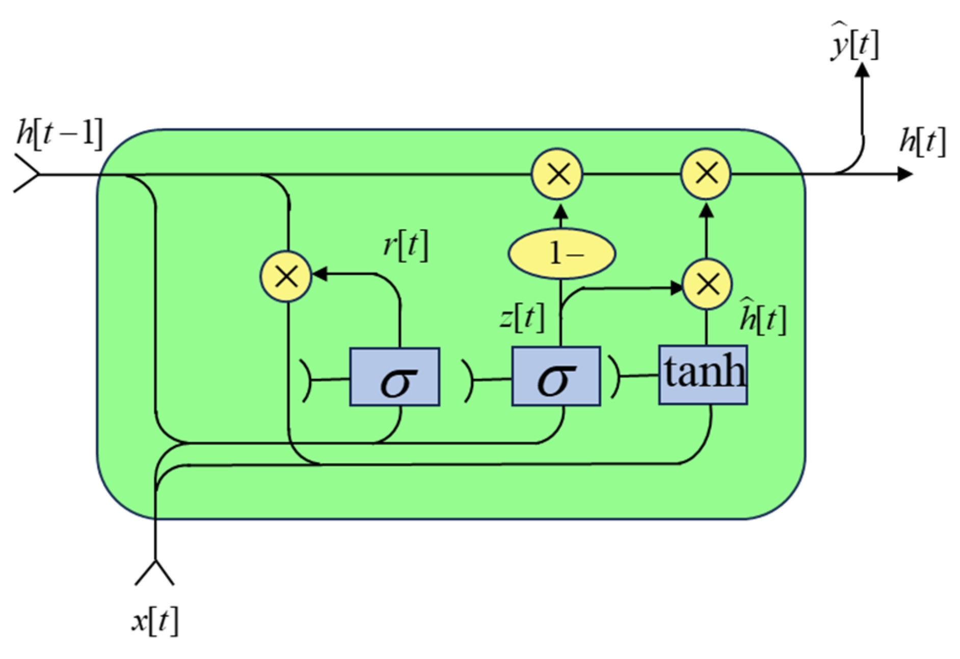
3.3. Gated Recurrent Unit

The Gated Recurrent Unit (GRU) is an RNN variant used to process and model sequential data [27]. Compared to the LSTM network, which has a more complex structure and more internal parameters, the GRU introduces a simplified architecture. By incorporating an update gate and a reset gate, the GRU maintains the ability to capture long-term dependencies in time series data while reducing the computational complexity. The detailed structure of the GRU is illustrated in Figure 4.

The update gate determines how much of the previous hidden state should be retained in the current hidden state. When its value is close to 1, more historical information is preserved; when it is close to 0, the model relies more on the current input. The reset gate controls the extent to which historical information influences the generation of the candidate hidden state; smaller values result in less influence from the past states. Together, these two gates effectively regulate the balance between memory retention and information forgetting, thereby enhancing the sequence modeling capability of the network. The computation process is as follows:

$$z_t=\sigma (W_z\cdot [h_{t-1},x_t])$$

(12)

$$r_t=\sigma (W_r\cdot [h_{t-1},x_t])$$

(13)

$${\tilde{h}}_t=\tanh (W\cdot [r_t\ast h_{t-1},x_t])$$

(14)

$$h_t=(1-z_t)\ast h_{t-1}+z_t\ast {\tilde{h}}_t$$

(15)

In the equation, $z_t$ and $r_t$ represent the update gate and reset gate, respectively; $\sigma$ is a nonlinear activation function. $W_z$, $W_r$, and $W$ are trainable weight parameters learned during the training process. ${\tilde{h}}_t$ denotes the candidate hidden state, and $h_t$ represents the output vector at time step t.

3.4. Focal Loss

Focal Loss [28] is a loss function designed to address the problem of class imbalance. It aims to mitigate the tendency of traditional cross-entropy loss to bias the model toward majority classes when dealing with imbalanced data. By introducing a tunable focusing factor, Focal Loss dynamically adjusts the weighting of each sample based on the difficulty of its prediction: it down-weights the loss contribution of easily classified majority-class samples and up-weights that of hard-to-classify minority-class samples. This mechanism reduces the influence of well-classified examples on the overall loss, thereby guiding the model to focus more on challenging and informative samples. As a result, it significantly improves the model’s learning capability and classification performance on imbalanced datasets. The formulation is as follows:

$$FL(p_t)=-{\alpha }_t{(1-p_t)}^{\gamma }\log (p_t)$$

(16)

In the equation, $p_t$ represents the predicted probability of the sample, $\alpha$ is the class weight coefficient used to balance the importance of samples, and $\gamma$ is the modulation factor that adjusts the weighting between easy and hard samples.

4. Experimental Validation

4.1. Dataset Introduction

The SCADA data used in this study were collected from a wind farm located in a northern province of China. The data pertain to grid-connected wind turbines of the same model, each with a rated capacity of 1.5 MW and employing a doubly fed induction generator (DFIG) configuration. The operational data and maintenance logs were recorded over the period from November 2016 to October 2017. The SCADA dataset includes 21 feature variables: the wind speed, active power on the grid side, generator speed, rotor speed, phase voltages (A, B, and C), phase currents (A, B, and C), power factor, grid frequency, yaw angle, blade pitch angle, nacelle temperature, gearbox oil temperature, stator winding temperature, low-speed shaft bearing temperature, high-speed shaft bearing temperature, and generator bearing temperatures (A and B). All variables have a temporal resolution of one minute. This study focuses on gearbox faults in wind turbines, with detailed fault information presented in

Table 1. Statistics for gearbox fault information.

No. WT	Fault Type	Fault Code
#32	/	0
#15, #14	High-Speed Shaft Temperature Exceeds Limit	1
#26, #7	Gearbox Lubricating Oil Overtemperature	2

.

4.2. Feature Selection

To balance model performance and computational efficiency, feature variable selection was conducted using the Pearson correlation coefficient, as described in Section 2.2. Since the generator speed is proportional to the rotor speed and the A, B, and C phase currents and voltages of the generator are essentially the same, only one from each group was selected as input. According to Table 1, the gearbox faults are categorized into two types: high-speed shaft anomaly and lubrication oil anomaly. As the directly monitored variables for these two fault types are the gearbox oil temperature and the high-speed shaft bearing temperature, other monitoring variables with a correlation coefficient greater than 0.2 with these two were selected as input features for the model. The selected feature variables used in this study are listed in

Table 2. SCADA feature variables used for model training.

/	Correlation Coefficient
Feature	Gearbox Oil Temperature	Gearbox High-Speed Shaft Bearing Temperature
Wind Speed	0.586	0.759
Active Power on Grid Side	0.557	0.722
Rotor Speed	0.582	0.771
Phase A Current	0.556	0.722
Nacelle Temperature	0.487	0.257
Gearbox Oil Temperature	1.000	0.936
Stator Winding Temperature	0.519	0.494
Gearbox Low-Speed Shaft Bearing Temperature	0.849	0.969
Gearbox High-Speed Shaft Bearing Temperature	0.936	1.000
Generator Bearing A Temperature	0.440	0.281
Generator Bearing B Temperature	0.797	0.682

.

During the dataset construction phase, the sliding window method was applied to process the SCADA data, with the window width set to 20. To construct labeled fault samples, this study first applied a sliding window approach to segment the SCADA data into continuous time slices. Early warning samples were identified using a preliminary rule-based detection model based on the lubricant oil temperature and high-speed shaft temperature. Gaps of up to 5 min between continuous warning signals were interpolated using mean values of all monitored parameters to preserve temporal continuity, and these segments were labeled as anomalous. To confirm the fault types, we cross-validated the early warning segments with the wind farm’s official maintenance logs. These logs recorded the time, scope, and cause of each maintenance activity, which enabled us to assign fault labels such as “gearbox lubricant over-temperature” or “high-speed shaft over-temperature.” Normal samples were selected from periods during which no faults were reported, based on maintenance records, and were also segmented using a sliding window method.

To ensure data consistency and avoid data leakage, all sample segments were normalized using the data from Turbine No. 32 as a unified baseline. Data from Turbines No. 26 and No. 15 were used for training, comprising 3537 normal samples, 190 lubrication oil fault samples, and 937 high-speed shaft fault samples, which were split into training and validation sets in a 7:3 ratio. Data from Turbines No. 14 and No. 7 were used as the test set, containing 5212 normal samples, 151 lubrication oil fault samples, and 950 high-speed shaft fault samples.

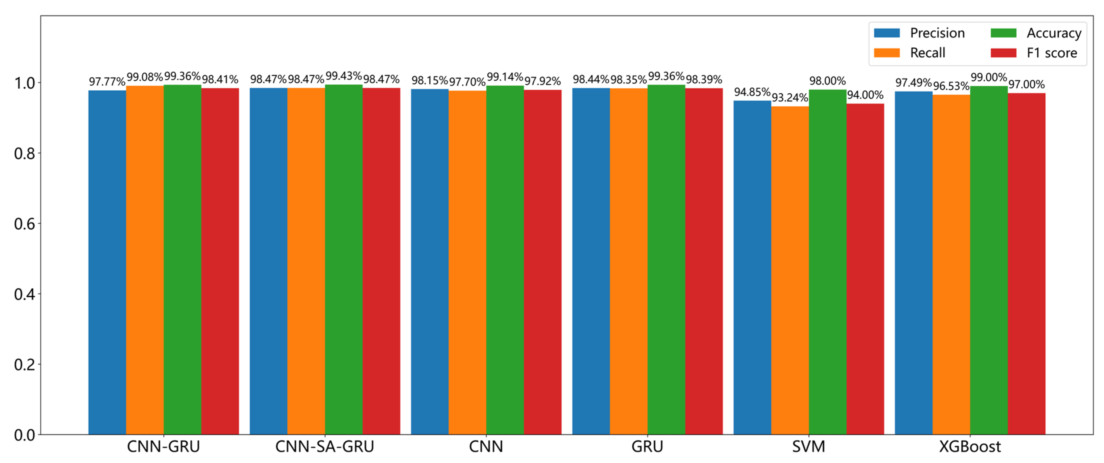
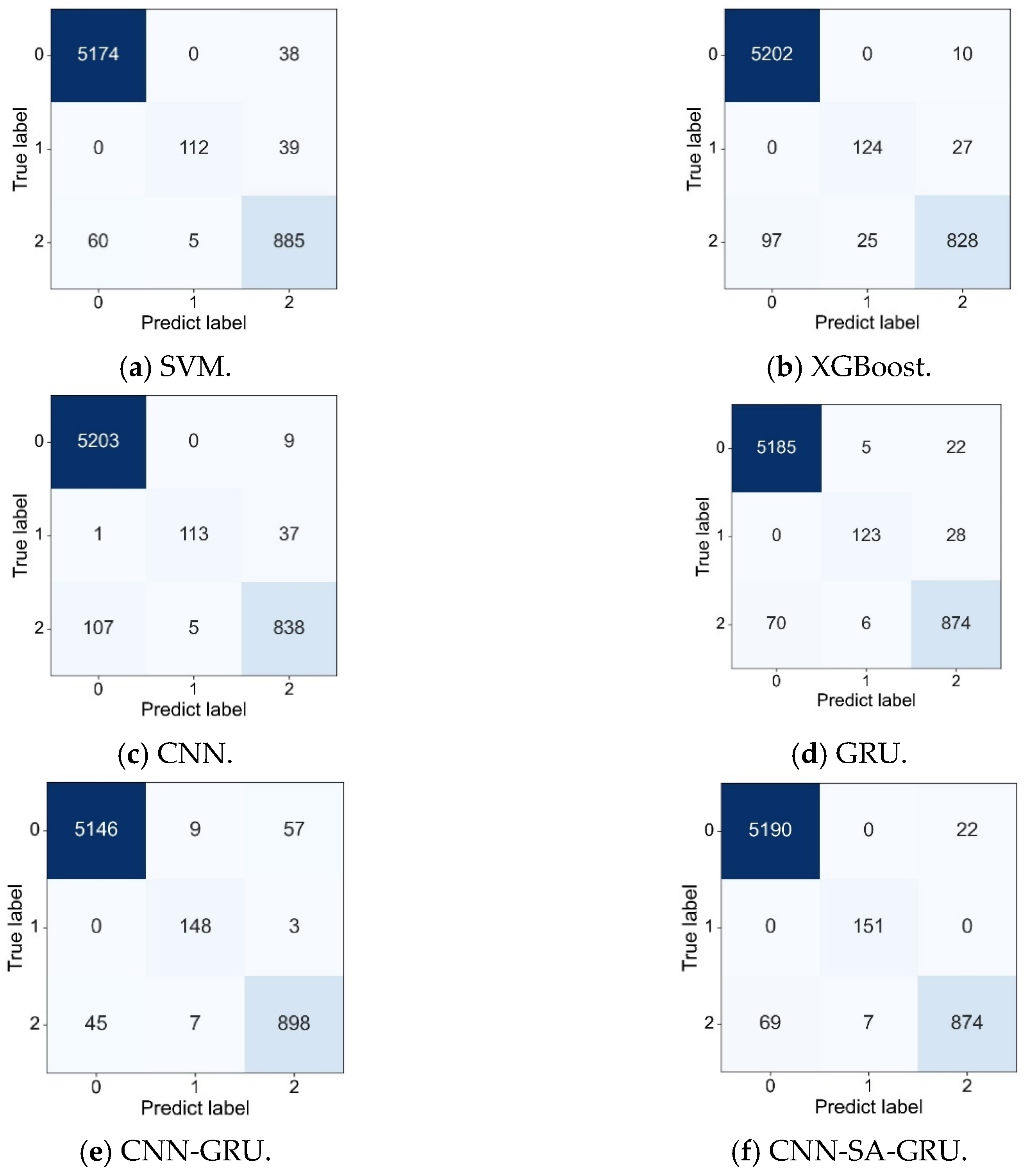
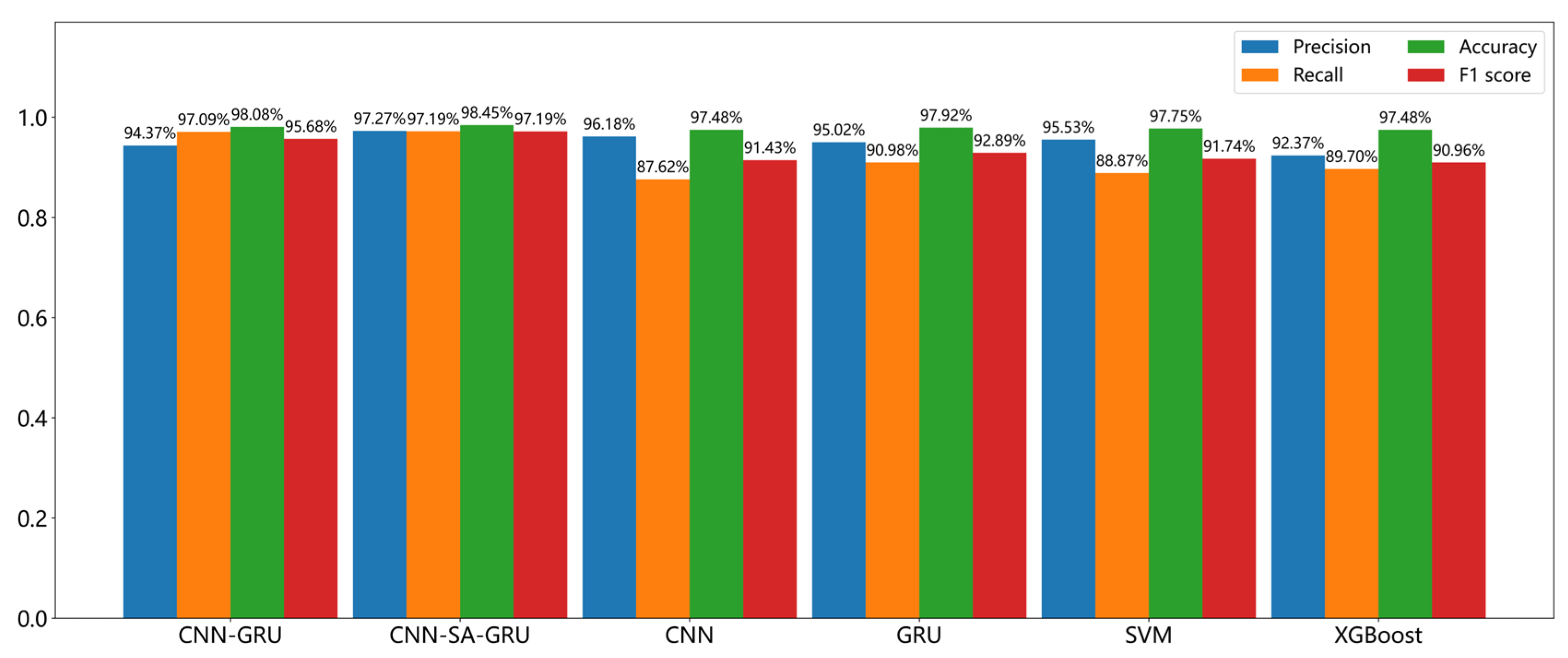
4.3. Comparison of Diagnostic Models

To further validate the effectiveness of the proposed model, six fault diagnosis models—CNN-SA-GRU, SVM, XGBoost, CNN, CNN-GRU, and LSTM—were constructed using the same dataset for comparative experiments. The hyperparameters of the proposed model are listed in

Table 3. Model hyperparameters.

CNN-SA-GRU	Kernel Size	Channels	Activation Function	Padding
Conv2d	3 × 3	128	Relu	1
MSConv2d	1 × 1,3 × 3	64,64	Relu	0,1
SA	/	64	/	/
Conv2d	3 × 3	64	Relu	1
BN	/	64	/	/
SA	/	64	/	/
Avg Pooling	2 × 2	/	/	0
GRU	/	128	Relu	/
GRU	/	128	Relu	/
Linear	/	64	Relu	/
Linear	/	3	Relu	/

. During training, the learning rate was set to 0.001, the number of training epochs was set to 200, the loss function used was Focal Loss, the optimizer was Adam, and the batch size was set to 128. The fault diagnosis results for different models on the validation set are shown in Figure 5.

The experimental results demonstrate that the proposed CNN-SA-GRU model outperforms the other models across four key metrics, precision, recall, accuracy, and F1 scores, exhibiting significant advantages. Specifically, in terms of precision, CNN-SA-GRU achieved 98.47%, representing an improvement of 0.32% to 3.62% over the baseline models. For recall, CNN-SA-GRU also achieved a leading performance of 98.47%, which, while slightly lower than that of the GRU model, still outperformed the other models by 0.12% to 5.23%. Regarding accuracy, CNN-SA-GRU achieved an outstanding result of 99.43%, surpassing the other models by 0.071% to 1.43%, demonstrating its high classification reliability. Notably, in the comprehensive evaluation metric F1 score, CNN-SA-GRU achieved the highest score of 98.47%, outperforming the second-best CNN-GRU model by 0.054% and surpassing the traditional machine learning methods SVM and XGBoost by 4.47% and 1.47%, respectively. These results clearly indicate that the CNN-SA-GRU model shows superior classification performance and stability in the task of wind turbine fault diagnosis, effectively balancing precision and recall.

To further verify the generalization ability and robustness of the proposed model, the trained model was transferred to Turbines No. 14 and No. 7 for cross-turbine performance testing, in order to evaluate its adaptability and reliability under different operating environments and conditions. The confusion matrices of different models for fault diagnosis are shown in Figure 6, and the evaluation metrics for each model are presented in Figure 7.

Based on the results of cross-turbine testing, the proposed CNN-SA-GRU model achieved precision and F1 scores of 98.45% and 97.19%, respectively. Compared with its performance on the validation set, the model experienced only slight decreases of 0.98% in precision and 1.28% in F1 score, significantly outperforming other models and demonstrating excellent generalization ability and stability.

In a horizontal comparison of different models on the test set, the CNN-SA-GRU model consistently delivered the best performance across all key metrics, including precision, recall, accuracy, and F1 scores. Compared with traditional machine learning methods, the proposed model showed a marked advantage: it improved in accuracy by 0.697% and 0.966% over SVM and XGBoost, respectively, and improved the F1 score by 5.45% and 6.22%. In terms of spatiotemporal feature extraction, the proposed model outperformed CNN and GRU, with improvements of 0.97% and 5.75% in accuracy and 0.52% and 4.297% in the F1 score, respectively. Although CNN-GRU combines the strengths of both CNN and GRU, its performance still fell short of the proposed model, with the accuracy and F1 score lower by 0.36% and 1.51%, respectively. These comparative results indicate that the proposed model, by introducing the Shuffle Attention mechanism, effectively integrates key information across channel and spatial dimensions in the feature maps, enabling fine-grained spatial feature extraction and significantly enhancing the model’s feature representation capacity. Overall, in terms of accuracy, the proposed model outperformed other baseline models by 0.36% to 0.97%, with an average improvement of 0.703%. In terms of F1 scores, the improvement ranged from 1.51% to 6.22%, with an average increase of 4.65%.

The experimental results confirm that the CNN-SA-GRU model exhibits strong adaptability and stability in cross-turbine testing. Its unique attention mechanism and hybrid network architecture effectively enhance the model’s capability in extracting spatiotemporal features and improving generalization performance. Compared with traditional methods and single-model approaches, the proposed model maintains high accuracy while reducing dependence on specific data sources, thereby validating its effectiveness.

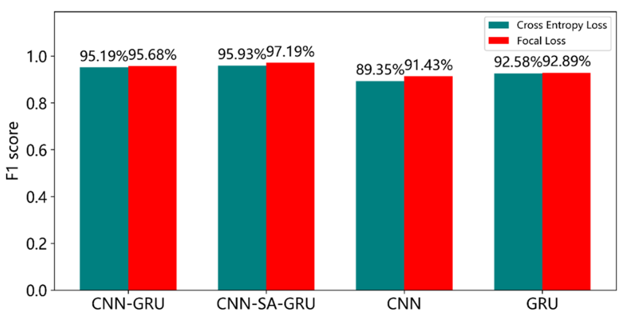
4.4. Performance Evaluation of Focal Loss

To further verify the effectiveness of the proposed Focal Loss in addressing class imbalance in wind turbine fault diagnosis, a comparative analysis was conducted on the diagnostic performance of four neural network models—CNN-GRU, CNN-SA-GRU, CNN, and GRU—under both the traditional cross-entropy loss function and Focal Loss. The evaluation focused on two key metrics: the accuracy and F1 score. The results are illustrated in Figure 8 and Figure 9.

After adopting Focal Loss as the loss function, improvements in accuracy were observed across the CNN-SA-GRU, CNN, and GRU models to varying degrees. Among them, the CNN model showed the largest increase, with a 0.71% improvement in accuracy, while the CNN-SA-GRU model achieved a 0.22% increase. On average, the four models experienced an accuracy improvement of 0.24%. Regarding the F1 score, all four models demonstrated significant gains. The CNN model achieved the highest improvement, with an increase of 2.08% in harmonic mean, followed by a 1.25% improvement in the CNN-SA-GRU model. The GRU model showed the smallest gain, with an increase of 0.31%. The average improvement across the four models in F1 score reached 1.03%. These results indicate that the proposed Focal Loss is well suited for addressing class imbalance in wind turbine fault diagnosis tasks.

5. Conclusions

This paper proposes a fault diagnosis model for wind turbine gearboxes based on CNN-SA-GRU and Focal Loss. First, a CNN-SA-GRU network was constructed: the CNN module was employed to extract local spatial features from SCADA data, while the Shuffle Attention mechanism effectively fused key information across channel and spatial dimensions, enabling fine-grained spatial feature extraction. The GRU module was then used to capture temporal dependencies in the data. Second, the Focal Loss function was introduced to address the class imbalance problem commonly found in fault samples. Finally, the model was validated using SCADA data collected from a wind farm located in a certain province in China. The proposed model was compared with five other baseline models. Experimental results demonstrate that the proposed method achieves superior diagnostic accuracy, generalization capability, and robustness. The main conclusions are as follows:

(1)

The proposed CNN-SA-GRU model effectively captures the spatiotemporal features in SCADA data. It achieved an accuracy of 98.45% and an F1 score of 97.19%, representing average improvements of 0.703% and 4.65%, respectively, over the baseline models. These results validate the model’s superiority in feature extraction and fault classification.

(2)

Neural network models based on Focal Loss can effectively mitigate the performance degradation caused by class imbalance in wind turbine gearbox fault samples. Compared with the traditional cross-entropy loss function, models using Focal Loss achieved an average improvement of 0.24% in accuracy and 1.03% in F1 score, demonstrating the effectiveness of Focal Loss in handling imbalanced classification problems.

Nevertheless, this method still has certain limitations and room for improvement:

(1)

Due to the limited types and quantities of fault samples, the proposed method was validated using only two types of fault data. Future research should explore a wider range of fault scenarios to enhance the robustness of the approach.

(2)

The hyperparameters of the proposed model were selected empirically without systematic optimization or sensitivity analysis. Future work could investigate the use of automated hyperparameter optimization methods to further improve model performance.

References

1. Bertling, L.; Ribrant, J. Survey of Failures in Wind Power Systems with Focus on Swedish Wind Power Plants 1997-2005. IEEE Trans. Energy Convers. 2007, 22, 167–173. [Google Scholar] [CrossRef]
2. Qiu, Y.; Feng, Y.; Sun, J.; Zhang, W.; Infield, D. Applying Thermophysics for Wind Turbine Drivetrain Fault Diagnosis Using SCADA Data. IET Renew. Power Gen. 2016, 10, 661–668. [Google Scholar] [CrossRef]
3. Corley, B.; Koukoura, S.; Carroll, J.; McDonald, A. Combination of Thermal Modelling and Machine Learning Approaches for Fault Detection in Wind Turbine Gearboxes. Energies 2021, 14, 1375. [Google Scholar] [CrossRef]
4. Shao, H.; Gao, Z.; Liu, X.; Busawon, K. Parameter-Varying Modelling and Fault Reconstruction for Wind Turbine Systems. Renew. Energy 2018, 116, 145–152. [Google Scholar] [CrossRef]
5. Zhang, C.; Hu, D.; Yang, T. Anomaly Detection and Diagnosis for Wind Turbines Using Long Short-Term Memory-Based Stacked Denoising Autoencoders and XGBoost. Reliability Engineering & System Safety 2022, 222, 108445. [Google Scholar] [CrossRef]
6. Wang, D.; Cao, C.; Chen, N.; Pan, W.; Li, H.; Wang, X. A Correlation-Graph-CNN Method for Fault Diagnosis of Wind Turbine Based on State Tracking and Data Driving Model. Sustain. Energy Technol. Assess. 2023, 56, 102995. [Google Scholar] [CrossRef]
7. Xiang, L.; Wang, P.; Yang, X.; Hu, A.; Su, H. Fault Detection of Wind Turbine Based on SCADA Data Analysis Using CNN and LSTM with Attention Mechanism. Measurement 2021, 175, 109094. [Google Scholar] [CrossRef]
8. Zhang, J.; Xu, B.; Wang, Z.; Zhang, J. An FSK-MBCNN Based Method for Compound Fault Diagnosis in Wind Turbine Gearboxes. Measurement 2021, 172, 108933. [Google Scholar] [CrossRef]
9. Zhang, K.; Tang, B.; Deng, L.; Liu, X. A Hybrid Attention Improved ResNet Based Fault Diagnosis Method of Wind Turbines Gearbox. Measurement 2021, 179, 109491. [Google Scholar] [CrossRef]
10. Zhang, Y.; Lv, Y.; Ge, M. Time–Frequency Analysis via Complementary Ensemble Adaptive Local Iterative Filtering and Enhanced Maximum Correlation Kurtosis Deconvolution for Wind Turbine Fault Diagnosis. Energy Rep. 2021, 7, 2418–2435. [Google Scholar] [CrossRef]
11. Ma, Z.; Zhao, M.; Luo, M.; Gou, C.; Xu, G. An Integrated Monitoring Scheme for Wind Turbine Main Bearing Using Acoustic Emission. Signal Process. 2023, 205, 108867. [Google Scholar] [CrossRef]
12. Schlechtingen, M.; Ferreira Santos, I. Comparative Analysis of Neural Network and Regression Based Condition Monitoring Approaches for Wind Turbine Fault Detection. Mech. Syst. Signal Process. 2011, 25, 1849–1875. [Google Scholar] [CrossRef]
13. Liu, J.; Yang, G.; Li, X.; Hao, S.; Guan, Y.; Li, Y. A Deep Generative Model Based on CNN-CVAE for Wind Turbine Condition Monitoring. Meas. Sci. Technol. 2023, 34, 035902. [Google Scholar] [CrossRef]
14. Zhang, G.; Li, Y.; Zhao, Y. A Novel Fault Diagnosis Method for Wind Turbine Based on Adaptive Multivariate Time-Series Convolutional Network Using SCADA Data. Adv. Eng. Inform. 2023, 57, 102031. [Google Scholar] [CrossRef]
15. Xiang, L.; Yang, X.; Hu, A.; Su, H.; Wang, P. Condition Monitoring and Anomaly Detection of Wind Turbine Based on Cascaded and Bidirectional Deep Learning Networks. Appl. Energy 2022, 305, 117925. [Google Scholar] [CrossRef]
16. Jiang, G.; He, H.; Yan, J.; Xie, P. Multiscale Convolutional Neural Networks for Fault Diagnosis of Wind Turbine Gearbox. IEEE Trans. Ind. Electron. 2019, 66, 3196–3207. [Google Scholar] [CrossRef]
17. Chen, B.; Xie, L.; Li, Y.; Gao, B. Acoustical Damage Detection of Wind Turbine Yaw System Using Bayesian Network. Renew. Energy 2020, 160, 1364–1372. [Google Scholar] [CrossRef]
18. López De Calle, K.; Ferreiro, S.; Roldán-Paraponiaris, C.; Ulazia, A. A Context-Aware Oil Debris-Based Health Indicator for Wind Turbine Gearbox Condition Monitoring. Energies 2019, 12, 3373. [Google Scholar] [CrossRef]
19. Liu, J.; Wang, X.; Xie, F.; Wu, S.; Li, D. Condition Monitoring of Wind Turbines with the Implementation of Spatio-Temporal Graph Neural Network. Eng. Appl. Artif. Intell. 2023, 121, 106000. [Google Scholar] [CrossRef]
20. Pang, Y.; He, Q.; Jiang, G.; Xie, P. Spatio-Temporal Fusion Neural Network for Multi-Class Fault Diagnosis of Wind Turbines Based on SCADA Data. Renew. Energy 2020, 161, 510–524. [Google Scholar] [CrossRef]
21. Feng, C.; Liu, C.; Jiang, D. Root Cause Localization for Wind Turbines Using Physics Guided Multivariate Graphical Modeling and Fault Propagation Analysis. Knowl.-Based Syst. 2024, 295, 111838. [Google Scholar] [CrossRef]
22. Wang, Z.; Jiang, X.; Xu, Z.; Cai, C.; Wang, X.; Xu, J.; Zhong, X.; Yang, W.; Li, Q. An Early Anomaly Detection of Wind Turbine Gearbox Based on SLFormer Neural Network. Ocean Eng. 2024, 311, 118925. [Google Scholar] [CrossRef]
23. Lei, J.; Liu, C.; Jiang, D. Fault Diagnosis of Wind Turbine Based on Long Short-Term Memory Networks. Renew. Energy 2019, 133, 422–432. [Google Scholar] [CrossRef]
24. Wang, T.; Yin, L. A Hybrid 3DSE-CNN-2DLSTM Model for Compound Fault Detection of Wind Turbines. Expert Syst. Appl. 2024, 242, 122776. [Google Scholar] [CrossRef]
25. Lecun, Y.; Bottou, L.; Bengio, Y.; Haffner, P. Gradient-Based Learning Applied to Document Recognition. Proc. IEEE 1998, 86, 2278–2324. [Google Scholar] [CrossRef]
26. Zhang, Q.-L.; Yang, Y.-B. SA-Net: Shuffle Attention for Deep Convolutional Neural Networks. In Proceedings of the ICASSP 2021–2021 IEEE International Conference on Acoustics, Speech and Signal Processing (ICASSP), Toronto, ON, Canada, 6–11 June 2021; pp. 2235–2239. [Google Scholar]
27. Tao, C.; Tao, T.; Bai, X.; Liu, Y. Wind Turbine Blade Icing Prediction Using Focal Loss Function and CNN-Attention-GRU Algorithm. Energies 2023, 16, 5621. [Google Scholar] [CrossRef]
28. Cai, J.; Wang, S.; Xu, C.; Guo, W. Unsupervised Deep Clustering via Contractive Feature Representation and Focal Loss. Pattern Recognit. 2022, 123, 108386. [Google Scholar] [CrossRef]
Figure 1. Flowchart of wind turbine gearbox fault diagnosis.
Energies 18 03696 g001
Figure 2. Model architecture of the CNN-SA-GRU network.
Energies 18 03696 g002
Figure 3. Shuffle Attention module.
Energies 18 03696 g003
Figure 4. The structure of the GRU.
Energies 18 03696 g004
Figure 5. Evaluation metrics of different models on the validation set.
Energies 18 03696 g005
Figure 6. Confusion matrices of different models.
Energies 18 03696 g006
Figure 7. Evaluation metrics of different models on the test set.
Energies 18 03696 g007
Figure 8. Accuracy of different models under various loss functions.
Energies 18 03696 g008
Figure 9. F1 scores of different models under various loss functions.
Energies 18 03696 g009