Assessing the Heat Transfer Modeling Capabilities of CFD Software for Involute-Shaped Plate Research Reactors

Abstract

The ongoing efforts to convert High-Performance Research Reactors (HPRRs) using Highly Enriched Uranium (HEU) to Low-Enriched Uranium (LEU) fuel require reliable thermal–hydraulic assessments of modified core designs. The involute-shaped fuel plates used in several major HPRRs present unique modeling challenges due to their compact core geometries and high heat flux conditions. This study evaluates the capability of three commercial CFD tools, STAR-CCM+, COMSOL, and ANSYS CFX, to predict cladding-to-coolant heat transfer using Reynolds-Averaged Navier–Stokes (RANS) methods within the thermal–hydraulic regimes of involute-shaped plate reactors. Broad sensitivity analysis was conducted across a range of reactor-relevant parameters using two turbulence models ($k-ϵ$ and $k-\omega$ SST) and different near-wall treatment strategies. The results were benchmarked against the Sieder–Tate correlation and experimental data from historic studies. The codes produced consistent results, showing good agreement with the empirical correlation of Sieder–Tate and the experimental measurements. The findings support the use of these commercial CFD codes as effective tools for assessing the thermal–hydraulic performance of involute-shaped plate HPRRs and guide future LEU core development.

1. Introduction

High-Performance Research Reactors (HPRRs) are characterized by compact cores and high-power densities, requiring accurate thermal–hydraulic predictions essential for both reactor safety and performance optimization. In this context, Computational Fluid Dynamics (CFD) provides a powerful tool to complement the traditional one-dimensional (1D) analysis methods. By resolving the three-dimensional nature of coolant flow and heat transfer within the fuel elements, CFD enables us to obtain a more detailed understanding of temperature distributions, flow perturbations, and potential hot spots, particularly important for reactors operating with narrow coolant channels and high-temperature heat fluxes like HPRRs.

Despite these advantages, the application of CFD to nuclear reactor safety remains limited by validation gaps, modeling assumptions, and variability in the predictive capabilities of different software packages. This is especially critical for HPRRs using complex geometries, such as involute-shaped fuel plates, or challenging thermal–hydraulic conditions, where curvature effects and localized flow phenomena are often simplified in the conventional thermal–hydraulic assessments. For such applications, it is imperative to demonstrate that commercial CFD codes can reliably reproduce key physical phenomena under HPRR-relevant conditions. To date, the evidence remains incomplete, especially for HPRRs employing involute-shaped fuel plates.

To address this gap, code-to-code comparisons serve as an essential step toward quantifying modeling uncertainties and understanding the differences introduced by solver algorithms, turbulence models, and near-wall treatments. This is particularly relevant for ongoing efforts to convert reactors from Highly Enriched Uranium (HEU) to Low-Enriched Uranium (LEU, ²³⁵U/U < 20 wt.%) fuel, where small design changes can significantly affect the thermal–hydraulic margins. Ensuring that CFD tools deliver consistent and trustworthy results across platforms is thus crucial for the design and licensing of future LEU cores.

Three HPRRs worldwide have a fuel element with involute-shaped fuel plates: the High Flux Isotope Reactor (HFIR) located at the Oak Ridge National Laboratory (ORNL), Tennessee, USA [1]; the High Flux Reactor (RHF) located at the Institut Laue-Langevin (ILL), Grenoble, France [2]; and the Research Neutron Source Heinz Maier-Leibnitz (FRM II) located at the Technical University of Munich (TUM), Garching, Germany [3]. Figure 1 shows the top views of these fuel elements for HFIR, RHF, and FRM II from left to right, respectively. The HFIR core contains two concentric fuel elements (inner and outer), while the RHF and FRM II cores each contain a single element. The use of involute-shaped fuel plates results in compact fuel elements and enables the generation of high neutron fluxes (i.e., Φ > 10¹⁴ n/cm²/s) and brilliances, making these reactors ideal for performing neutron scattering experiments and radioisotope production.

The fuel plates—from 1.27 to 1.36 mm thick—are spot-welded to the concentric side plates and contain HEU fuel dispersed in aluminum. The coolant channels between the plates are narrow (1.27–2.2 mm) and approximately 60–90 cm long, with downward coolant flow. HFIR and FRM II use light water; RHF uses heavy water. Table 1 summarizes the nominal characteristics of coolant flow and heat generated in the fuel elements of these reactors.

Because the plates are shaped as involutes, the coolant channels maintain a constant thickness from the inner to the outer edges of the element. All the coolant channels are nominally identical, and all the fuel plates experience similar irradiation conditions. These features are particularly advantageous for thermal–hydraulics analyses, as analyzing a single plate and its adjacent coolant channels can effectively characterize the behavior of the entire fuel element. Additionally, the constant channel thickness supports the use of a simplified thermal–hydraulic modeling approach for the involute-shaped channels, treating them as simple rectangular channels heated on both sides. However, this approach ignores the flow variations caused by channel curvature and does not consider the offset in heat deposition between the concave and convex sides of the plate. These simplifications typically yield conservative results and have historically been utilized for Steady-State Thermal–Hydraulic (SSTH) safety calculations [4].

Figure 1. From bottom left to bottom right: top view of the HFIR, RHF, and FRM II fuel elements (close to the true proportions). Partially reproduced from [5].

Figure 1. From bottom left to bottom right: top view of the HFIR, RHF, and FRM II fuel elements (close to the true proportions). Partially reproduced from [5].

Table 1. Nominal thermal–hydraulic parameters of fuel elements with involute-shaped plates. Partially reproduced from [5].

Parameters	HFIR [6]	RHF [7]	FRM II [8]
Thermal power (MW)	85	58	20
Coolant type	H2O	D2O	H2O
Average coolant velocity (m/s)	15.5	17	15.9
Inlet/outlet bulk coolant temperature (°C)	49/69	30/50	37/53
Inlet/outlet pressure (bar)	33.3/25.72	14/4	8.8/2.3
Reynolds number range (within channel)	70–95k	50–125k	100–210k
Prandtl number range (within channel)	2.5–3.6	2.9–6.8	2.8–4.6
Peak heat flux (W/cm2)	<400	340	389

Table 1. Nominal thermal–hydraulic parameters of fuel elements with involute-shaped plates. Partially reproduced from [5].

Parameters	HFIR [6]	RHF [7]	FRM II [8]
Thermal power (MW)	85	58	20
Coolant type	H2O	D2O	H2O
Average coolant velocity (m/s)	15.5	17	15.9
Inlet/outlet bulk coolant temperature (°C)	49/69	30/50	37/53
Inlet/outlet pressure (bar)	33.3/25.72	14/4	8.8/2.3
Reynolds number range (within channel)	70–95k	50–125k	100–210k
Prandtl number range (within channel)	2.5–3.6	2.9–6.8	2.8–4.6
Peak heat flux (W/cm2)	<400	340	389

The conversion of involute-shaped plate reactors to LEU fuel is underway. Each reactor’s conversion must result in a design that ensures safety, while maintaining acceptable performance levels. This requires the development of new core designs with modifications to the fuel materials and the core and plate geometry, which are specific to each of the three reactors. Consequently, the comprehensive assessment of the thermal hydraulics and safety margins for the new LEU fuel core designs is essential.

While higher-fidelity approaches, such as Large Eddy Simulations (LES) and Direct Numerical Simulations (DNS) [9], offer greater detail in the resolution of the field variables, Reynolds-Averaged Navier–Stokes (RANS) methods provide a balance between accuracy and computational efficiency, making them well-suited for engineering analyses. RANS methods have been successfully employed in basic CFD analyses of involute-shaped plate thermal–hydraulic performance [5,7,10,11,12,13]. However, CFD based analyses have not yet been accepted by regulators for the safety analysis of research rectors with involute-shaped fuel plates.

This paper aims to assess the cladding-to-coolant heat transfer modeling capabilities of the RANS methods for thermal hydraulic conditions relevant to involute-shaped plate research reactors. Channel flow analyses using RANS, LES, and DNS have already been studied and presented elsewhere, for example [14,15,16,17,18,19,20]. However, a literature review indicates that channel flow analyses combining narrow channels, high heat flux, and high Reynolds and Prandtl numbers, in addition to modeling the temperature-dependent thermo-physical properties of liquid-phase coolant, remain largely unexplored. By focusing on the unique thermal–hydraulic conditions of involute-shaped fuel plates, this work augments the existing channel flow analyses to include conditions that have not been previously reported.

Simulations for a blind comparison were independently conducted by three groups of participating organizations, each using a different CFD code based on a distinct underlying algorithm. The codes used were as follows: STAR-CCM+ 16.04 [21], which utilizes the cell-centered finite volume method (FVM); ANSYS CFX 2022.R2 [22], which uses the vertex-based FVM; and COMSOL 5.6 [23], which applies the finite element method (FEM).

Although the complex geometries of the involute-shaped fuel plates were not explicitly analyzed in this work, the conducted assessment used generalized models for a comprehensive sensitivity study spanning the thermal–hydraulic conditions of the HFIR, RHF, and FRM II fuel elements. The simulations used two commonly applied turbulence models ($k-ϵ$ and $k-\omega$ SST) combined with two near-wall modeling approaches. The results include comparisons with a well-established Nusselt number correlation, cross-code consistency checks, and validation against the experimental data. This work represents an important step in establishing confidence in commercial CFD tools for the thermal–hydraulic analysis of involute-shaped plate fuel elements and of new high-performance nuclear reactors.

2. Generalized Heat Transfer Modeling

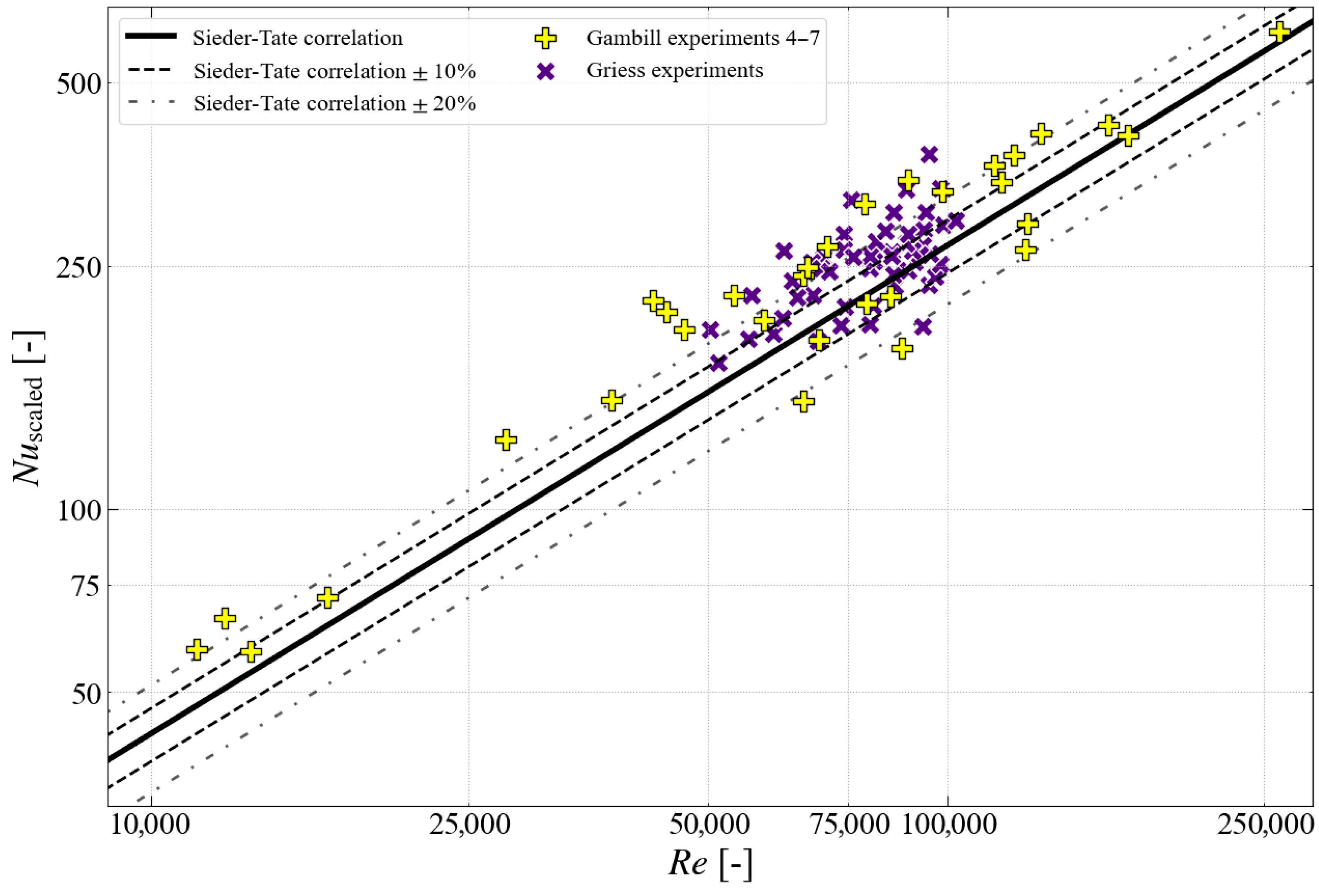
2.1. Experimental Results Used for Comparison

Heat transfer experiments were conducted in the 1960s by Gambill and Bundy [24] and Griess [25] to support the thermal–hydraulic design of HFIR. These experiments focused on evaluating heat transfer coefficients for water flowing through heated aluminum and nickel specimens with a thin coolant channel. Of these two studies, Gambill and Bundy’s work spanned a wider range of input parameters relevant to this analysis. Geometry details were provided for all the cases investigated by Gambill and Bundy, but specific operating conditions were defined for only one case (later referred to as Test #7). For the remaining cases, only ranges of operating conditions were provided, and they reported the dependency of the scaled Nusselt number $Nu$, on the Reynolds number Re, or ${Nu}_{scaled}\left(Re\right)$.

In these two experimental studies [24,25], the Sieder–Tate correlation [26] was used as a reference for comparison with the experimental data. It is defined by the following equation:

$$Nu=0.027{Re}^{0.8}{Pr}^{1/3}{\left({\displaystyle \frac{{\mu }_b}{{\mu }_w}}\right)}^{0.14}$$

(1)

where $Pr$ is the Prandtl number and $\mu$ is the dynamic viscosity. The indices b and w indicate if $\mu$ is evaluated with respect to bulk ($b$) or wall ($w$) temperatures. Sieder–Tate correlation is valid for bulk Prandtl numbers ${0.7\le Pr}_b\le \mathrm{16,700}$ and Reynolds numbers $Re\ge \mathrm{10,000}$ [27], which encompasses the normal operation conditions of involute-shaped plate reactors.

The scaled Nusselt number derived from this is defined by the following equation:

$${Nu}_{scaled}={\displaystyle \frac{{\left(Nu\right)}_b}{{\left(Pr\right)}_b^{1/3}}}{\left({\displaystyle \frac{{\mu }_w}{{\mu }_b}}\right)}^{0.14}$$

(2)

The scaling of experimental data by the Prandtl number and the viscosity ratio, as shown in Equation (2), enables the straightforward comparison of the Nu versus Re dependence for the coolant under different temperature conditions. Nevertheless, such non-dimensionalization is not reversible without more detailed information about the data.

The main results from both studies are reproduced in Figure 2. In this plot, the data from Gambill and Bundy represent the averages over the entire length of the tested specimens, while Griess’s study provides local values. As noted by Griess [25], approximately 74% of the total of 86 points from the two experiments are situated above the Sieder–Tate correlation, with about 56% falling within the ±20% range. The experiments conducted afterwards, including [28] and the more recent [29], compared the measured data to the Sieder–Tate or Dittus–Boelter correlations [30], showing a similar spread of data. However, the ranges of Re and Nu in the work of Gambill and Bundy and that of Griess extend beyond those in the newer studies, which makes their data more applicable to involute-shaped plate reactors.

While the comparison with the Sieder–Tate correlation is not intended as a recommendation for use in the safety analysis of research reactors with involute-shaped plate fuel elements, the correlation itself is based on a broad set of experimental data and remains relevant for the design and analysis of research reactors [24,28,31], making it applicable to this work.

2.2. Generalized Model Description

The clear and concise representation of Gambill and Bundy’s experimental data (i.e., the use of a scaled Nusselt number) supports the use of numerical models that focus only on relevant experimental parameters. It makes the explicit modeling of the entire test section unnecessary for broad sensitivity analysis. To minimize the computational cost, a simplified abstract geometry model, termed the “generalized model”, was created for each code. The model was based on fully developed flow conditions, avoiding the regions near the inlet, outlet, and channel corners. Due to the differences in code capabilities, some aspects of the generalized model vary between codes.

The geometry of the generalized model is a cuboid with the edge sized at 1 mm × 1 mm × 0.5 times the channel thickness. It represents a small section of the heated channel away from the inlet and the side edges of the channel. Figure 3 illustrates the location of the numerical domain in the coolant channel and a typical domain of the generalized model created in STAR-CCM+ and COMSOL. The heated wall is marked in red, while the symmetry boundary conditions applied on the sides of the model are shown in blue. On the surface opposing the heated wall, a symmetry boundary condition was applied to mark the middle of the channel. This assumption makes the model equivalent to a very wide, thin channel. To replicate long heated channels, such as those present in involute-shaped plate reactors and those studied by Gambill and Bundy, periodic boundary conditions were applied on the inlet and outlet surfaces of the domain, indicated in orange. This approach allows for fully developed conditions within a short numerical domain when a scaled temperature profile from the outlet is applied on the inlet of the domain [21]. Such scaling is only valid when a constant temperature or a constant heat flux is applied on the wall parallel to the main flow direction, as in the current simulations with a constant heat flux.

Since ANSYS CFX does not have a straightforward method for modeling periodic boundary conditions to solve heated fluid flow problems, an extended domain was implemented instead. This approach allows for the full development of velocity and temperature boundary layers within the computational domain. The symmetry planes were maintained on the sides of the model, consistent with the models used in the other two codes. The length of the heated section of the model was equal to approximately 80 hydraulic diameters, with an additional unheated section at the inlet being 30 hydraulic diameters long. This extension allows for the flow to develop before entering the heated section.

A recent numerical study by Popov et al. [9] evaluated the validity of the flat parallel channel approximation used in the generalized model and assessed its applicability to involute-shaped plates. Through DNS of full involute coolant channels, partial sections, and flat parallel channels, they showed that the bulk flow behavior in the involute channels closely matches that of the parallel channels, with noticeable differences limited to the corner regions. Consequently, the geometric simplifications used in the present work are deemed appropriate for the simulations of the flow in the main part of the channel, and the results remain highly relevant for involute-shaped channels.

Of interest for this work were two different eddy viscosity turbulence models, namely variants of the $k-ϵ$ and $k-\omega$ SST turbulence models under the RANS method. These turbulence models were selected because they are widely used by the CFD community for various engineering applications. For both the turbulence models, two types of near-wall treatment were considered: one with a high $y^{+}$ near-wall mesh ($y^{+}=40$) and one with a low $y^{+}$ near-wall mesh ($y^{+}=0.6$). A low $y^{+}$ near-wall mesh with $y^{+}<1$ allows for directly resolving near-wall flows without relying on wall functions. In contrast, a high $y^{+}$ near-wall mesh with $y^{+}>30$ prompts the use of the wall functions, which interpolate near-wall flow and temperature behavior using empirical relationships. The evaluation of $y^{+}$ for all the codes is based on the first cell thickness.

The implementation of the $k-\omega$ SST model in all three codes relies on the same reference [32]. However, the implementation of the $k-ϵ$ model was specific to each code. The realizable $k-ϵ$ two-layer model [33] was specific to STAR-CCM+. Two formulations of $k-ϵ$ turbulence models were utilized in the simulations conducted in COMSOL, a standard $k-ϵ$ based on [34] and a low Re $k-ϵ$ based on [35], for the simulation with the high $y^{+}$ near-wall mesh and the low $y^{+}$ near-wall mesh, respectively. This is because for the version of COMSOL software used in this work, there is no version of the $k-ϵ$ turbulence model that is applicable to both ranges of the near-wall mesh sizes studied. For ANSYS CFX, the standard $k-ϵ$ turbulence model was used with scalable wall functions [22]. The temperature wall functions implemented in STAR-CCM+ and ANSYS CFX follow Kader’s law [36]. Since COMSOL is an FEM code, its temperature wall function implementation differs. The definitions of these functions can be found in the code’s manual [37] and in [38].

The temperature- and pressure-dependent properties of water were used in these simulations. The STAR-CCM+ models used the built-in International Association for the Properties of Water and Steam (IAPWS) material model database [39], while for COMSOL and ANSYS CFX, the Python IAPWS library [40] was used to externally create the temperature-dependent polynomials used for all of the analyzed cases.

A structured, hexahedral mesh was used in all the conducted simulations. For the simulations conducted here and for the flows expected in the coolant channels of the involute-shaped plate research reactors, the flow is primarily unidirectional. Therefore, a structured mesh aligned with the flow direction introduces less numerical diffusion compared to that of an unstructured mesh. Because the $y^{+}$ of the near-wall cell is influenced by the variable material properties, determining the exact mesh size in advance was challenging. To maintain consistency across the codes and reduce variations in the results, the near-wall mesh size was iteratively determined for each case to keep the $y^{+}$ values within 5% of the target values of 0.6 and 40. This was achieved using the internal loop algorithm (STAR-CCM+) or an external Python 3 script (COMSOL and ANSYS CFX).

Depending on the analyzed case and the targeted $y^{+}$ value, a different number of cells through the thickness of the channel, i.e., normal for the heated wall, were needed to obtain mesh-independent results. For the cases with a low temperature gradient between the wall and the coolant, for which wall functions were used ($y^{+}=40$), mesh sensitivity analyses confirm that as few as five layers of cells through the thickness of the modeled half channel were sufficient to obtain converged results. For the cases with a near-wall mesh size $y^{+}=0.6$ and a high temperature gradient between the wall and the coolant, as many as 50 layers of cells were required. As few as three cells across the other two directions were sufficient to obtain converged results. The overall cell count in such models for STAR-CCM+ and COMSOL was below 1000. Since the ANSYS CFX models did not rely on a cyclic boundary interface, the meshes used in ANSYS CFX consisted of up to 660,000 cells, depending on the hydraulic diameter and the target value of $y^{+}$.

To verify equivalence between the models using the periodic boundary conditions and the extended length models used in ANSYS CFX, several simulations were performed in STAR-CCM+ with both the types of modeling techniques. The results from these additional simulations closely matched those obtained with the equivalent periodic boundary interface models (predicted wall temperature within 0.5%). Thus, it was concluded that the generalized models used in all the three codes are numerically equivalent.

To generate a simulation matrix encompassing the historical work performed by Gambill and Bundy, three different values of hydraulic diameter, bulk velocity, coolant temperature, and pressure, and four different values of the onset of nucleate boiling ratio (ONBR) were considered [41]. Note that the concept of the ONBR was used in this study only to ensure that the generated cases led to single-phase liquid flows. The Bergles-Rohsenow correlation was used to calculate the wall heat flux values used as the input for the simulations that matched a specific ONBR under a given pressure, resulting in twelve distinct values of wall heat flux. This selection of parameters and their values created a set of 648 distinct cases.

The combination of two turbulence models and two near-wall mesh sizes applied to the 648 configurations of input variables resulted in a total of 2592 cases simulated in each code. The list of independent parameters for the simulation matrix is presented in

Table 2. Input variables and their values used in sensitivity analysis. Partially reproduced from [5].

Quantity	Unit	Values
Independent variables
Hydraulic diameter	m	0.00254, 0.00376, 0.0044
Bulk coolant velocity	m/s	5, 10, 18
Bulk coolant temperature	°C	10, 30, 50, 70, 90, 110
Pressure	MPa	0.4, 2.0, 4.0
ONBR	-	1.05, 1.2, 2.0, 5.0
	Dependent variables
Range of resultant heat fluxes	W/cm2	26–1700
Range of Re	-	10,000–300,000
$\mathrm{Range} \mathrm{of} {Pr}_b$	-	1.6–10

, along with the resultant range of heat fluxes on the wall, Re and ${Pr}_b$.

2.3. Results from the Generalized Model Parameter Study

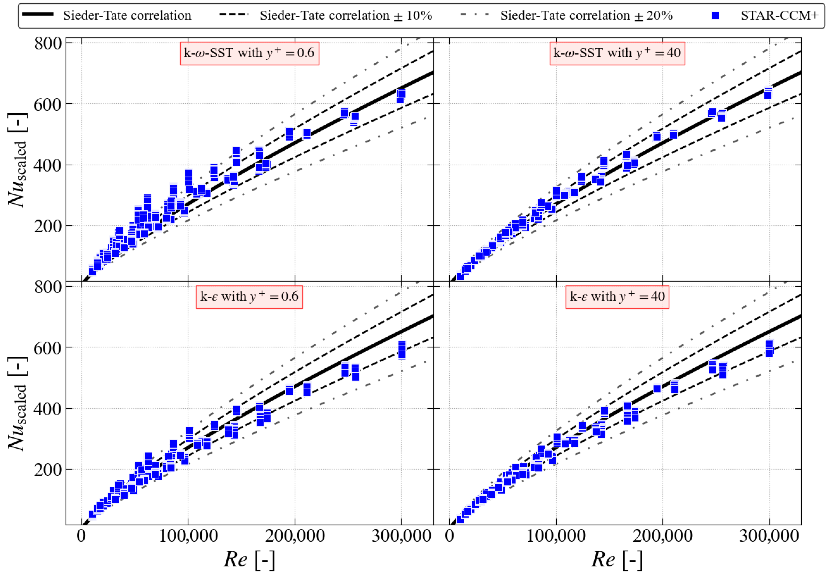
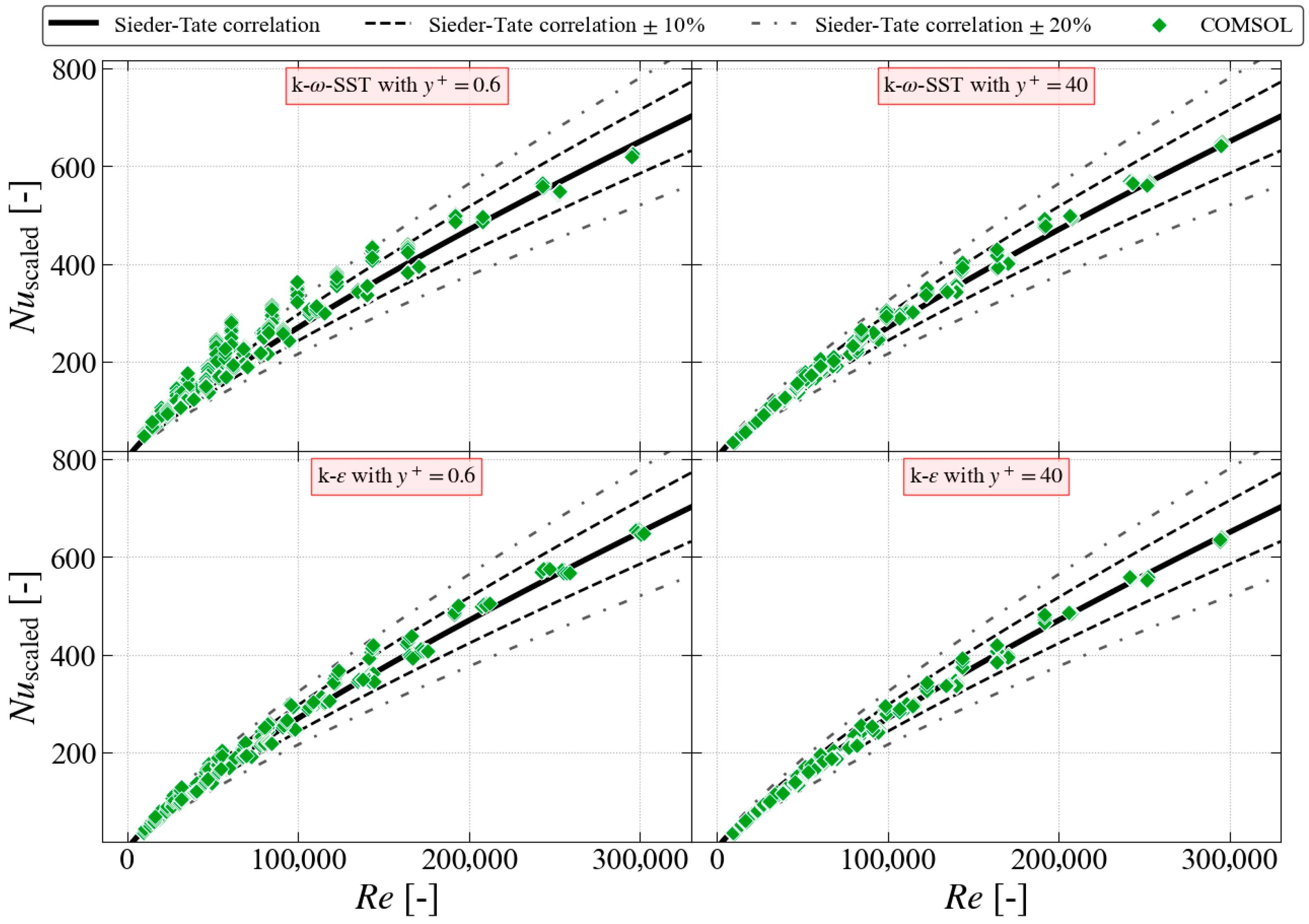
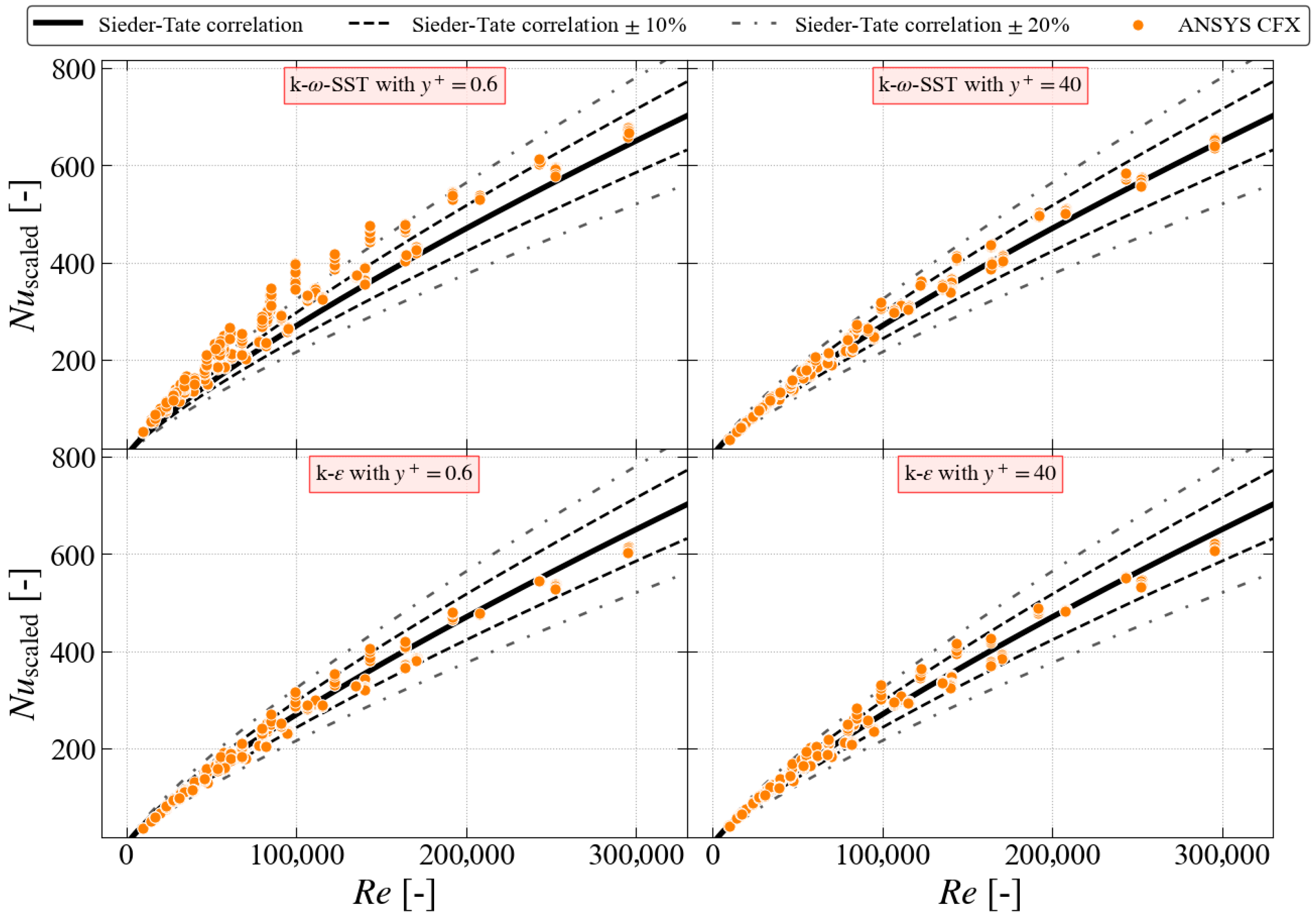
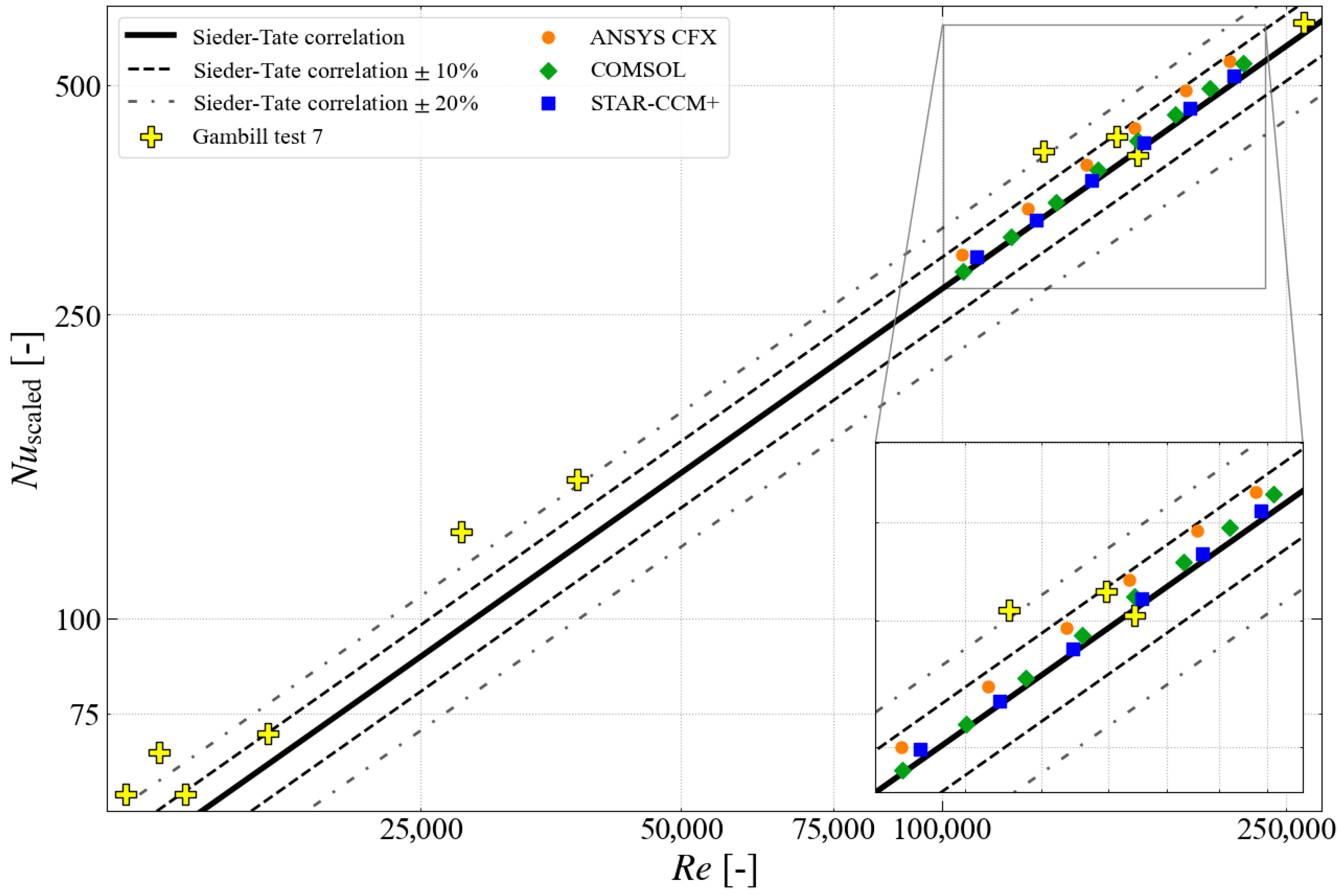
2.3.1. Comparison with Sieder–Tate Correlation

Figure 4, Figure 5 and Figure 6 display the results of ${Nu}_{scaled}\left(Re\right)$ obtained using STAR-CCM+, COMSOL, and ANSYS CFX, respectively. Each figure consists of four subplots, with the top rows containing the data for $k-\omega$ SST and the bottom rows presenting the data for the $k-ϵ$ turbulence models. The subplots on the left present the results obtained with a low $y^{+}$ near-wall mesh with $y^{+}=0.6$, while those on the right display the results from a high $y^{+}$ near-wall mesh with $y^{+}=40$.

For STAR-CCM+ and COMSOL, which use periodic boundary conditions, the bulk data were extracted at the outlet cross section of the domain. For ANSYS CFX, the data were taken from a plane located in the middle of the heated section, or 40 hydraulic diameters from each end to minimize the inlet and outlet effects [42].

To facilitate the comparison of the large data sets generated by the different codes using two turbulence models and two near-wall meshing approaches, the Sieder–Tate correlation is included in each plot, following the data analysis strategy from Gambill and Bundy [24]. It should be noted that this correlation is a fit to the experimental data, and the proximity of the CFD data points to this line does not imply the greater accuracy of the numerical model. Rather, it serves as a benchmark for indirectly comparing the performance of the different codes. The dashed and dash-dotted lines illustrate ±10% and ±20% deviations from the correlation, respectively. The relative number of data points falling within these bands are presented in

Table 3. STAR-CCM+ Nusselt number predictions compared to Sieder–Tate correlation.

	Agreement Within ±10%	Agreement Within ±20%
$k-\omega$ SST, low $y^{+}$ near-wall mesh	51%	72%
$k-\omega$ SST, high $y^{+}$ near-wall mesh	94%	100%
$k-ϵ$, low $y^{+}$ near-wall mesh	71%	94%
$k-ϵ$, high $y^{+}$ near-wall mesh	91%	100%

,

Table 4. COMSOL Nusselt number predictions compared to Sieder–Tate correlation.

	Agreement Within ±10%	Agreement Within ±20%
$k-\omega$ SST, low $y^{+}$ near-wall mesh	51%	71%
$k-\omega$ SST, high $y^{+}$ near-wall mesh	94%	100%
$k-ϵ$, low $y^{+}$ near-wall mesh	90%	100%
$k-ϵ$, high $y^{+}$ near-wall mesh	93%	99%

and

Table 5. ANSYS CFX Nusselt number predictions compared to Sieder–Tate correlation.

	Agreement Within ±10%	Agreement Within ±20%
$k-\omega$ SST, low $y^{+}$ near-wall mesh	34%	61%
$k-\omega$ SST, high $y^{+}$ near-wall mesh	89%	100%
$k-ϵ$, low $y^{+}$ near-wall mesh	88%	100%
$k-ϵ$, high $y^{+}$ near-wall mesh	87%	99%

.

The results obtained with STAR-CCM+ are shown in Figure 4. The data points from the simulations using the $k-\omega$ SST turbulence model with a low $y^{+}$ near-wall mesh (top left) present a higher spread compared to the results obtained from models using the wall functions on a high $y^{+}$ near-wall mesh (top right). The results obtained with the realizable $k-ϵ$ turbulence model show similar trends to those obtained with the $k-\omega$ SST turbulence model. However, the spread of the individual data points from the models with a low $y^{+}$ near-wall mesh (bottom left) is smaller than that from the corresponding model using $k-\omega$ SST turbulence (top left). A similar spread of the data is observed for the model using high $y^{+}$ near-wall mesh (bottom right) as for the corresponding model using $k-\omega$ SST turbulence (top right).

The quantitative comparison of these results obtained using STAR-CCM+ is presented in Table 3. For both the turbulence models and the high $y^{+}$ near-wall meshing, over 90% of the data points fall within ±10% of the Sieder–Tate correlation, with all the data points falling within ±20% of the correlation. However, not all the data points from the simulations using low $y^{+}$ near-wall mesh fall within ±20% of the Sieder–Tate correlation, with 72% and 94% for $k-\omega$ SST and $k-ϵ$, respectively.

The results obtained using COMSOL are presented in Figure 5. It is important to note that the COMSOL results for the high $y^{+}$ near-wall mesh were obtained with higher-order elements, while linear elements were used in the simulations with a low $y^{+}$ near-wall mesh. Second-order shape functions were used for the solution of the velocity and temperature fields. The linear shape functions were used for the pressure field. This increase in the order of shape functions was necessary due to the deteriorated performance observed in the models using the high $y^{+}$ near-wall mesh. The use of higher-order elements significantly increases the runtime of the simulations. More details about the discretization schemes used in COMSOL can be found in the user manual [43].

The spread of the Nusselt number predictions is wider for the $k-\omega$ SST model with the low $y^{+}$ near-wall mesh (top left) as compared to the spread of the data obtained using high $y^{+}$ near-wall (top right) mesh model predictions. For the $k-ϵ$ turbulence model using the low $y^{+}$ near-wall mesh (bottom left), the spread of Nusselt number predictions is narrower than for the corresponding $k-\omega$ SST calculations. For the results obtained using the $k-ϵ$ turbulence model and the high $y^{+}$ mesh, the spread is very small.

The quantitative comparison of these results is presented in Table 4. For both the turbulence models and the high $y^{+}$ near-wall meshing, over 90% of the data points fall within ±10% of the Sieder–Tate correlation, with over 99% of data points falling within ±20% of the correlation. This is also true for $k-ϵ$ with a low $y^{+}$ near-wall mesh. However, only 71% of the data fall within ±20% of the Sieder–Tate correlation for $k-\omega$ SST with a low $y^{+}$ near-wall mesh.

The results obtained with ANSYS CFX are shown in Figure 6. For the $k-\omega$ SST turbulence model (top subplots), similar observations can be made as for the other two codes. Namely, there is a larger spread of data for the models using a low $y^{+}$ near-wall mesh than for the models using a high $y^{+}$ near-wall mesh. The results from the simulations using the $k-ϵ$ turbulence model (bottom subplots) do not show such a difference between the two mesh densities used. This is caused by the specific implementation of this turbulence model in the software. The standard $k-ϵ$ model in ANSYS CFX has a lower limit for $y^{+}$ at 11.06 [22]. This means that for near-wall meshes denser than this, the solver will use $y^{+}$ = 11.06 regardless of its actual value. Consequently, the predictions made by the models with a low $y^{+}$ near-wall mesh are nearly identical to those obtained with the models with a high $y^{+}$ near-wall mesh.

The quantitative comparison of the results from ANSYS CFX simulations is presented in Table 5. For both the mesh densities and the standard $k-ϵ$ turbulence model, as well as the high $y^{+}$ near-wall mesh and the $k-\omega$ SST turbulence model, nearly 90% of the data points were within ±10% of Sieder–Tate correlation, and nearly all the data points were within ±20% of the correlation. For the $k-\omega$ SST turbulence model, 34% and 61% of the data points were within ±10% and within ±20% of the Sieder–Tate correlation, respectively.

2.3.2. Comparison with Experimental Data

Given that all three codes use similar implementations of $k-\omega$ SST based on the same reference [32], while different variants of $k-ϵ$ were used (realizable, low Re, and standard), the remaining discussion in this section is focused primarily on the results obtained using the $k-\omega$ SST turbulence model. The results obtained with this turbulence model, as predicted by STAR-CCM+, COMSOL, and ANSYS CFX, were compared against the experimental data from Gambill and Bundy [24], as well as Griess [25], as shown in Figure 7 and Figure 8 for the low $y^{+}$ and high $y^{+}$ near-wall meshes, respectively. This is not only to directly perform code-to-code comparison, but also to understand the level of consistency between the numerical results and the data sets from the two experimental studies.

Since only the geometries of the samples were known in the work by Gambill and Bundy, but the initial conditions were defined within ranges, the direct comparison of the CFD results with the individual experimental data points was not possible for the generalized model simulation. Therefore, the plot of the individual experimental data points, presented previously in Figure 2, was omitted. Instead, respective envelopes were drawn for both the experimental data sets against the background of the numerical data. In addition, the Sieder–Tate correlation is also shown, with the dashed and dash-dotted lines representing ±10% and ±20% deviations from the correlation, respectively.

Analogous to Figure 2, it is shown in Figure 7 and Figure 8 that both the experimental data sets tend to predict a larger Nusselt number compared to the Sieder–Tate correlation. The numerically obtained data points using the $k-\omega$ SST turbulence model and the low $y^{+}$ near-wall mesh are, like the experimental data, more abundant above the Sieder–Tate correlation line (Figure 7). For most of the cases, the numerical data points stay within the envelopes of the experimental data.

Figure 8 presents the numerical data obtained with the use of a high $y^{+}$ near-wall mesh and the $k-\omega$ SST turbulence model compared to the same envelope of experimental results and the Sieder–Tate correlation. Regarding the numerical data, especially for STAR-CCM+, ANSYS CFX presents a substantially smaller spread than the experimental data. This is also true for the COMSOL-generated results for Re > 50,000.

Despite the differences in the implementation of underlying equations in the codes and the modeling techniques used, the results obtained with STAR-CCM+, COMSOL, and ANSYS CFX exhibit a high degree of consistency in the trends and spread of data. A notable similarity is the larger data spread observed for the low $y^{+}$ near-wall mesh compared to the high $y^{+}$ near-wall mesh results.

The results predicted by the models with the high $y^{+}$ near-wall mesh tend to align more closely with the Sieder–Tate correlation. This holds true across the entire spectrum of Reynolds numbers studied for STAR-CCM+, COMSOL, and ANSYS CFX.

Models with a low $y^{+}$ near-wall mesh, which resolve the flow in the viscous sublayer, are generally considered more accurate. However, this work does not determine which turbulence model or near-wall meshing approach aligns more closely with real-world data at the level of individual data points. Further comparisons with the experimental data or simulations using higher fidelity modeling techniques are required to answer this question. To partially address this need, the following section performs the comparison of the numerical predictions to the results of the single fully defined experimental setup studied by Gambill and Bundy.

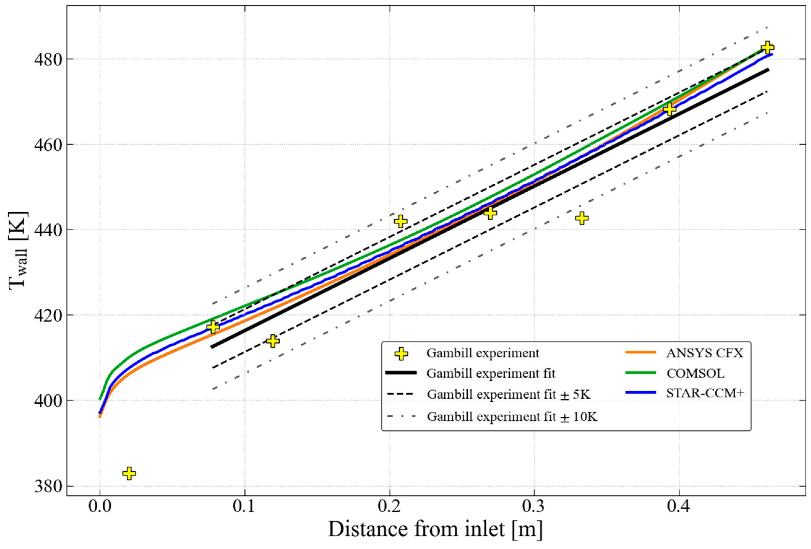
3. Explicit Modeling of Gambill and Bundy Test #7

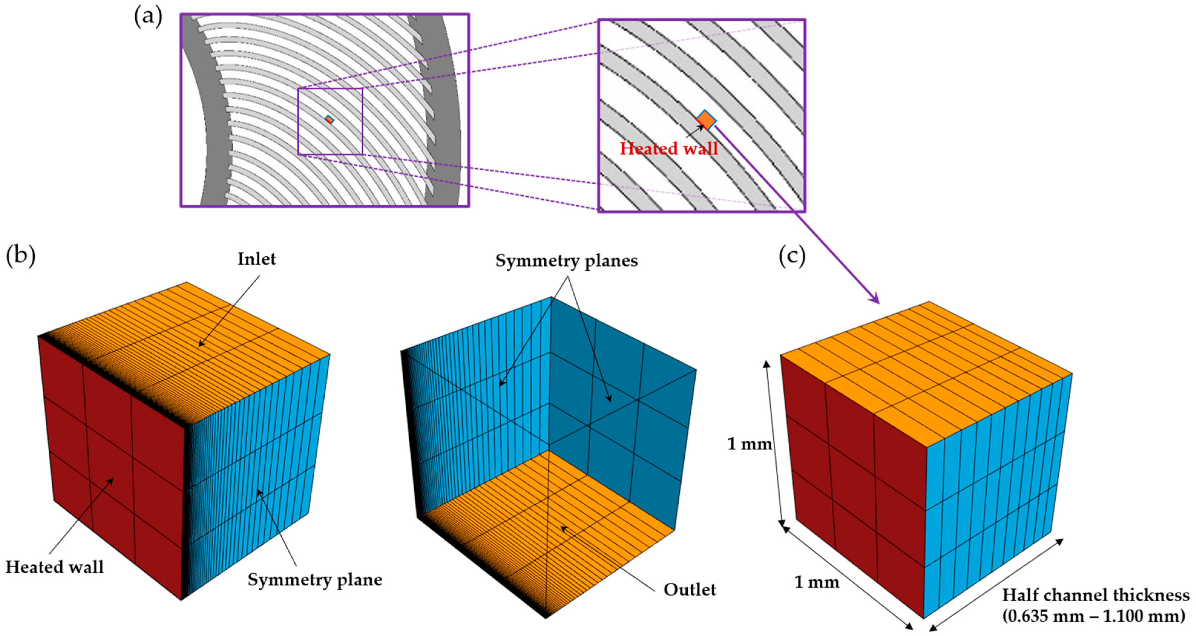
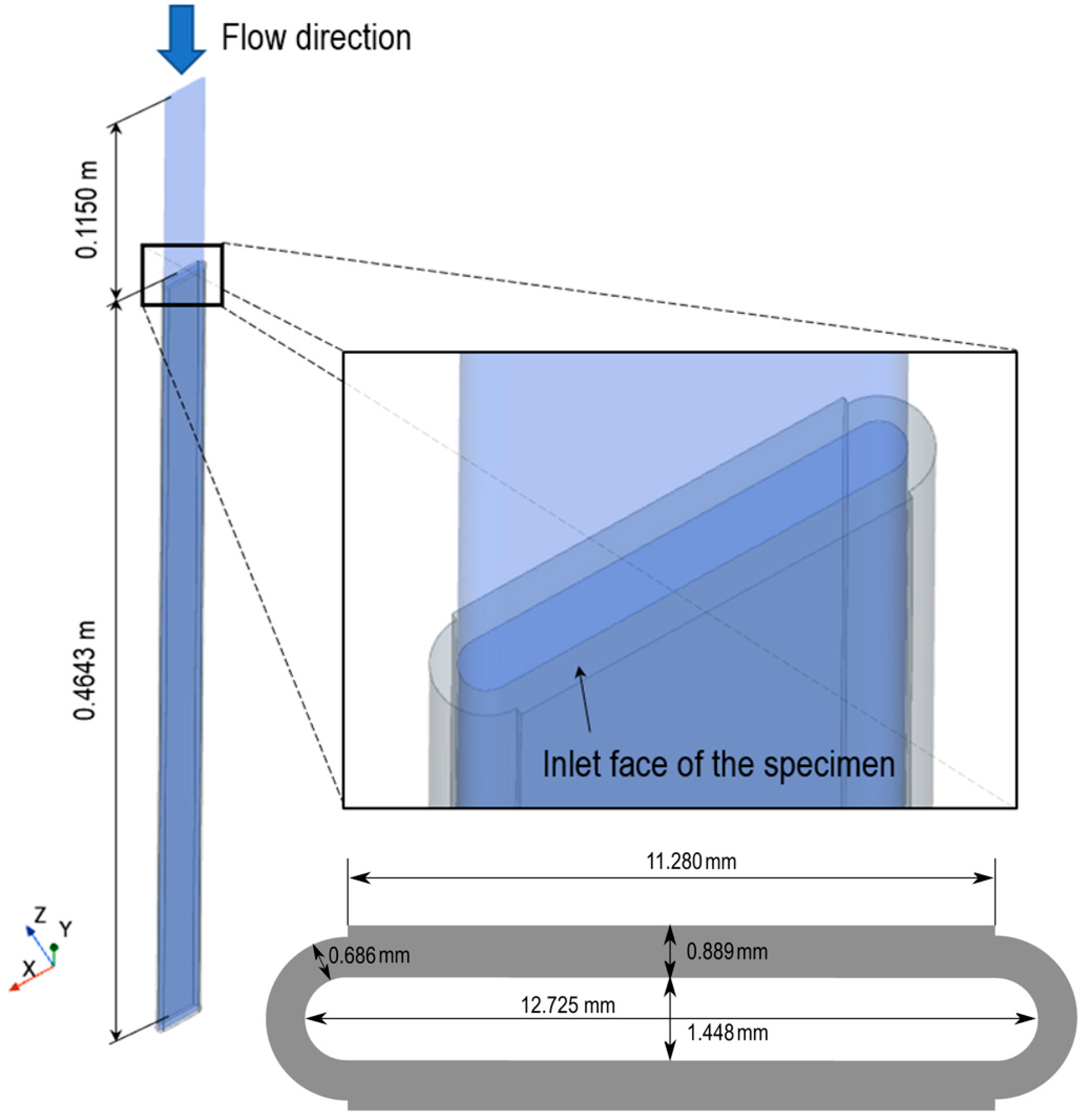
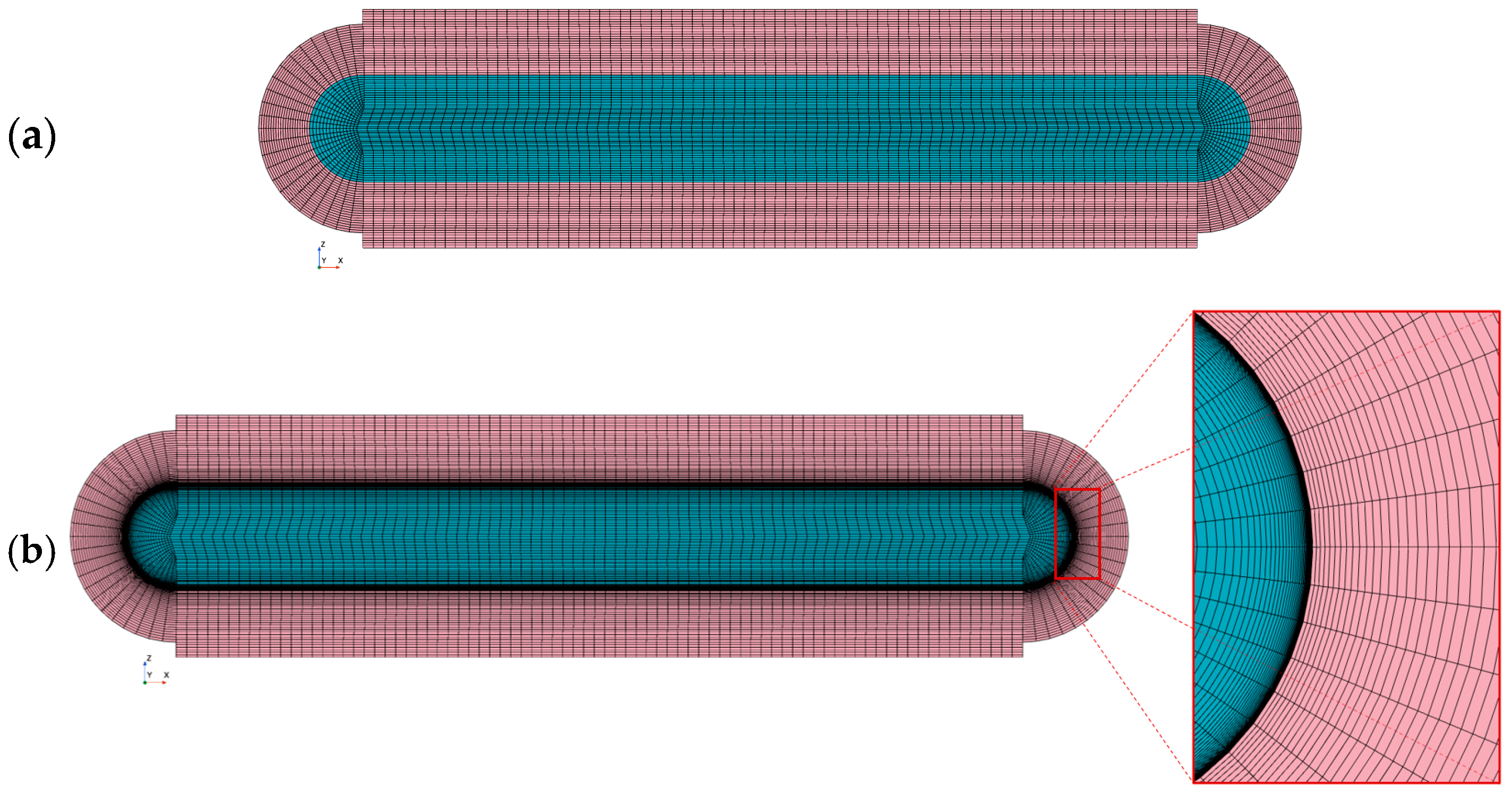
3.1. Test #7 Model Description

The models of Gambill and Bundy Test #7 were developed for all three codes using the same geometry file. The assumed dimensions of the model are shown in Figure 9. The detailed inlet conditions were not specified in [24], so a fully developed flow at the inlet to the heated section was used in the models. This was achieved by adding a flow development inlet section that had a length equivalent to approximately 40 hydraulic diameters [11,42]. The experimental setup allowed for conductive heat losses near the inlet, which were of unknown magnitude. These were ignored in the simulations, and adiabatic boundary conditions were assumed on the external walls of the model. Consequently, the comparison of the numerical results with the experimental measurements focused primarily on the section where flow and thermal boundary layers had developed.

While preliminary efforts have been made previously to model this experiment [5,12], the current work focused on the $k-\omega$ SST turbulence model and near-wall meshing approaches for the three codes. This particular turbulence model was selected for comparison due to its demonstrated good agreement in the code-to-code comparison between STAR-CCM+, COMSOL, and ANSYS CFX, as observed for the generalized model in Section 2. Also, as previously stated, the implementation of the $k-\omega$ SST turbulence model was found to be the more consistent across all the codes when compared to the other turbulence models investigated.

Figure 10 presents two typical mesh distributions in the channel cross section developed for the STAR-CCM+ models, featuring near-wall mesh sizes of $y^{+}$ < 1 (low $y^{+}$) and $y^{+}$ > 30 (high $y^{+}$), respectively. Similar mesh densities were used across the other codes to satisfy these $y^{+}$ requirements. Although the changing material properties of the heated coolant caused variations in $y^{+}$ along the domain, the conditions of $y^{+}$ < 1 and $y^{+}$ > 30 were consistently maintained throughout each model’s domain to ensure the appropriate handling of the near-wall region by each code. The mesh sensitivity study was conducted independently for all three codes. The total cell counts for the high and low $y^{+}$ models were 3.3 M and 6.6 M in STAR-CCM+, 4.7 M and 6.5 M in ANSYS CFX, and 1.2 M (second order) and 5.6 M in COMSOL, respectively.

These models used the same water properties as those in the generalized model simulations. A constant thermal conductivity of 218 W/m·K was assumed for the solid component of the model (Aluminum 1100 alloy) based on [44], as it is not expected to vary significantly within the temperature range considered [45]. The inlet bulk velocity was set to 15.7 m/s, with a coolant bulk temperature of 68.5 °C at the inlet. A volumetric heat source was used in the solid part of the models to generate the total power equivalent to the experimentally measured value of 100 kW.

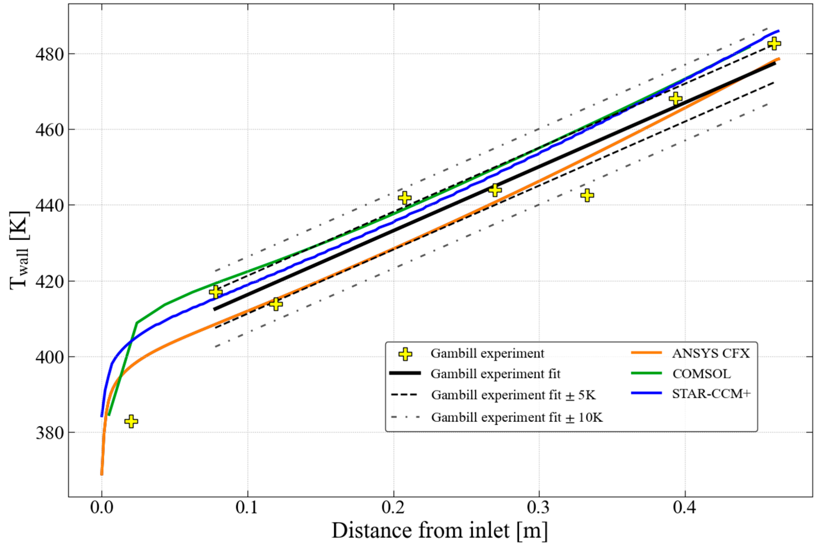
3.2. Results from the Simulations of Test #7

The results of the experiments included the temperatures on the interface of the specimen with the coolant for a single run of Test #7, as well as averaged (single value per entire specimen) ${Nu}_{scaled}\left(Re\right)$ for each test. The former data set allows for the direct comparison of the numerical data versus the experimental ones, while the latter only allows for a qualitative assessment. Both the comparisons were attempted in this work.

Figure 11 presents a comparison of wall temperature variation along the axial distance from the channel inlet, as obtained with the three different codes using the $k-\omega$ SST turbulence model with the low $y^{+}$ near-wall mesh against the experimental data. The simulated results of all the codes exhibit good consistency with the experimental data, especially away from the channel inlet. The plot also features a linear fit to the experimental data, ignoring the data point near the inlet. The numerically obtained data remains within ±10 K of this fit for all the codes, with the ANSYS CFX data and most of the STAR-CCM+ data staying within ±5 K of the fit.

In Figure 12, a similar plot is presented, but for the numerical data obtained using the $k-\omega$ SST turbulence model with the high $y^{+}$ near-wall mesh that relies on wall functions. The numerical data obtained using the three codes stayed reasonably close to the linear fit of the experimental data (without the near-inlet point) for the entire length of the specimen, with the predicted temperature remaining within ±10 K. This difference is not significantly greater than the spread of the experimental data.

Figure 13 presents a comparison of the numerical results obtained with all the investigated codes using the models with a low $y^{+}$ near-wall mesh with the experimental data obtained by Gambill, as well as the Sieder–Tate correlation using the ${Nu}_{scaled}\left(Re\right)$ format. A similar plot is presented for models with a high $y^{+}$ near-wall mesh in Figure 14. Note that the numerical results represent the local data along the axial distance of the sample, while each experimental data point represents the average data from a separate test. Thus, the explicit comparison of that data set is not possible. Nevertheless, the validity of the presented comparison was proven by Griess, as discussed in [25] and shown in Figure 2.

The CFD results in Figure 13, obtained using all the codes, predict a higher Nusselt number than that predicted by the Sieder–Tate correlation. The results obtained using COMSOL and STAR-CCM+ are within ±10% of the Sieder–Tate correlation. The data points from ANSYS CFX are within ±20% of the Sieder–Tate correlation. It should be noted that the discrepancy, in terms of percentages, between the code predictions of the Nusselt number is greater than that for the wall temperature predictions shown previously. This is because the Nusselt number is directly related to the temperature rise at the wall. By focusing on wall temperature predictions, rather than the temperature rise from bulk fluid, the relative discrepancy in terms of percentages is reduced.

The simulation results obtained using a high $y^{+}$ near-wall mesh are shown in Figure 14. For all three codes, the data points fall within ±10% of the Sieder–Tate correlation. ANSYS CFX predicted values higher than the Sieder–Tate correlation. The results from STAR-CCM+ closely follow the Sieder–Tate correlation, with a slight overprediction. The COMSOL predictions were lower than the Sieder–Tate correlation. These results are consistent with the ones presented for the generalized model simulations.

4. Summary

In the first part of this work (Section 2), the commercial codes STAR-CCM+, COMSOL, and ANSYS CFX were used to evaluate the performance of two widely used turbulence models, $k-ϵ$ and $k-\omega$ SST, in a sensitivity analysis of a generalized geometry representing a section of a thin, heated rectangular channel. By varying the channel thicknesses, the inlet coolant velocity, the bulk temperature, the pressure, and the wall heat flux, a total of 648 distinct cases per code, turbulence model, and near-wall mesh resolution were evaluated. The range of the parameters enveloped the ranges of inputs used by Gambill and Bundy in their experiments, as well as the ranges representative of nominal operational conditions in involute-shaped plate reactors.

The trends observed in the form of scaled Nusselt numbers as a function of the Reynolds numbers predicted by various codes closely matched one another, especially for the case with the $k-\omega$ SST turbulence model and a low $y^{+}$ near-wall mesh size $y^{+}=0.6$. The individual data points obtained using the models with a low $y^{+}$ near-wall mesh show a wider spread than the data points obtained using the high $y^{+}$ near-wall mesh for all the three codes used with the $k-\omega$ SST turbulence model (Figure 4, Figure 5 and Figure 6). This spread is within the observed spread of the experimental data reported by Gambill and Bundy, as well as in the data reported by Griess [24,25].

The data obtained using the high $y^{+}$ near-wall mesh for both the studied turbulence models tend to be grouped close to the Sieder–Tate correlation. However, the Sieder–Tate correlation is a fit to several experimental data sets with significant spread. Thus, having a smaller spread around that curve is not an indication of a numerical model being more accurate. It only indicates consistency with the correlation.

Similar observations could be made for the results obtained with the use of the $k-ϵ$ turbulence model for the COMSOL (Figure 5) and STAR-CCM+ (Figure 4) codes. For ANSYS CFX, the implementation of the $k-ϵ$ turbulence model for meshes with a low $y^{+}$ is made by truncating the solver $y^{+}$ to 11.06 in the code. Thus, for the simulations in ANSYS CFX using the $k-ϵ$ turbulence model, the results obtained with the model with a low $y^{+}$ near-wall mesh mimicked those obtained with the models using a high $y^{+}$ near-wall mesh (Figure 6). The use of $k-\omega$ SST turbulence model is advised for ANSYS CFX when resolving the flow in the viscous sublayer is of interest.

The results obtained with various turbulence models in these commercial codes using a near-wall mesh size of $y^{+}=40$ tend to predict lower Nusselt numbers than those obtained with the models using a low $y^{+}$ near-wall mesh (except for ANSYS CFX and the $k-ϵ$ turbulence model). Consequently, higher wall temperatures will usually be calculated when using models with a high $y^{+}$ near-wall mesh than those calculated with models using a low $y^{+}$ near-wall mesh ($y^{+}=0.6$). These results tend to match the Sieder–Tate correlation better.

In the second part of this work (see Section 3), the numerical models of a single specific test from the Gambill and Bundy experiments were analyzed. The predicted temperatures on the wall were compared to the experimental data. Despite the differences in code implementations, all the codes were able to predict the temperature on the wall in the region of interest with satisfactory accuracy, i.e., within ±10 K for both the low and high $y^{+}$ near-wall meshes.

The non-dimensional data from the simulations, ${Nu}_{scaled}\left(Re\right)$, were within ±20% from the Sieder–Tate correlation for the models with a low $y^{+}$ near-wall mesh ($y^{+}$ < 1), as presented in Figure 13. For the models with a high $y^{+}$ near-wall mesh ($y^{+}$ > 30), the non-dimensional data were within ±10% of the Sieder–Tate correlation for the three commercial codes tested (see Figure 14).

At this stage of the work, further analysis is needed to determine which combination of turbulence model and near-wall treatment most accurately represents reality. The results of the three codes agree well with each other and the experimental data in the form of heat transfer coefficient and wall temperature. The data largely represents the heat transfer conditions of the three involute-shaped plate reactors.

This study demonstrates that the commercially available CFD tools, STAR-CCM+, COMSOL, and ANSYS CFX, can produce consistent and credible results for heat transfer analysis in the coolant channel thicknesses and thermal hydraulic conditions relevant to HPRRs, e.g., for reactors with fuel elements consisting of involute-shaped fuel plates. Despite the differences in solver framework and turbulence model implementation, the agreement with the historical experimental data and across the codes reinforces the reliability of RANS-based CFD approaches for the engineering analysis of HPRRs. This work represents a significant step toward validating the use of commercial CFD software for supporting LEU core conversion in HPRRs. As the nuclear community increasingly relies on high-fidelity tools to guide design decisions, robust cross-code benchmarking, such as that presented here, will remain essential to ensure the safe and efficient advancement of research reactors.

References

1. Cheverton, R.; Sims, T. HFIR Core Nuclear Design; ORNL-4621; Oak Ridge National Laboratory (ORNL): Oak Ridge, TN, USA, 1971. [Google Scholar]
2. Calzavara, Y.; Fuard, S.; Bergeron, A. Evaluation of Measurements Performed on the French High Flux Reactor (RHF), Revision 2; RHF-FUND-RESR-001 CRIT; Institut Laue-Langevin: Grenoble, France; Argonne National Laboratory: Lemont, IL, USA, 2011. [Google Scholar]
3. Reiter, C.; Bergeron, A.; Bonete-Wiese, D.; Kirst, M.; Mercz, J.; Schönecker, R.; Shehu, K.; Ozar, B.; Puig, F.; Licht, J.; et al. A Low-Enriched Uranium (LEU) option for the conversion of FRM II. Ann. Nucl. Energy 2023, 183, 3. [Google Scholar] [CrossRef]
4. Hilvety, N.; Chapman, T. HFIR Fuel Element Steady State Heat Transfer Analysis; ORNL-TM-1903; Oak Ridge National Laboratory: Oak Ridge, TN, USA, 1967. [Google Scholar]
5. Bojanowski, C.; Bergeron, A.; Licht, J. Involute Working Group—Validation of CFD Turbulence Models for Steady-State Safety Analysis; ANL/RTR/TM-19/5; Argonne National Laboratory: Lemont, IL, USA, 2020. [Google Scholar]
6. Martin Marietta Energy Systems, Inc. Summary of HFIR Design Parameters For 85 MW Operation; ORNL/RRD/INT-55; Oak Ridge National Laboratory: Oak Ridge, TN, USA, 1989. [Google Scholar]
7. Thomas, F.; Calzavara, Y.; Guyon, H.; Tentner, A.; Bergeron, A. Thermo-Hydraulique d’une Lame RHF; Rapport RHF n414; Institut Laue Langevin: Grenoble, France, 2012. [Google Scholar]
8. Gysler; Sperber; Ehrich. Thermohydraulische Kernauslegung 3B 0320.0007; Bericht Nr. A1C-1301735-1; Siemens AG—Bereich Energieerzeugung (KWU): Erlangen, Germany, 1996. [Google Scholar]
9. Popov, E.L.; Mecham, N.J.; Bolotnov, I.A. Direct Numerical Simulation of Involute Channel Turbulence. ASME J. Fluids Eng. 2024, 146, 081301. [Google Scholar] [CrossRef]
10. Travis, A.R.; Ekici, K.; Freels, J.D. Simulating High Flux Isotope Reactor Core Thermal-Hydraulics via Interdimensional Model Coupling; Oak Ridge National Laboratory: Oak Ridge, TN, USA, 2014. [Google Scholar]
11. Bojanowski, C.; Bergeron, A.; Sitek, M.; Licht, J. Involute Working Group—Validation of CFD Turbulence Models for Steady-State Safety Analysis of Corner Geometry; ANL/RTR/TM-20/3; Argonne National Laboratory: Lemont, IL, USA, 2021. [Google Scholar]
12. Shehu, K.; Bojanowski, C.; Bergeron, A.; Petry, W.; Reiter, C. First Steps to Coupled Hydraulic and Mechanical Calculations within a Parameter Study to Define Possible Core Designs for the Conversion of FRMII. EPJ Web Conf. 2021, 247, 08011. [Google Scholar] [CrossRef]
13. Breitkreutz, H. Coupled Neutronics and Thermal Hydraulics of High Density Cores for FRM II; Technical University of Munich: München, Germany, 2011. [Google Scholar]
14. Kim, J.; Moin, P. Transport of Passive Scalars in Turbulent Channel Flow. In NASA Technical Memorandum 8946; National Aeronautics and Space Administration (NASA): Washington, DC, USA, 1987. [Google Scholar]
15. Kawamura, H.; Abe, H.; Matsuo, Y. DNS of turbulent heat transfer in channel flow with respect to Reynolds and Prandtl number effcts. Int. J. Heat Fluid Flow 1999, 20, 196–207. [Google Scholar] [CrossRef]
16. Abe, H.; Antonia, R.A. Relationship between the heat transfer law and the scalar dissipation function in a turbulent channel flow. J. Fluid Mech. 2017, 830, 300–325. [Google Scholar] [CrossRef]
17. Sergio, P.; Modesti, D. Direct numerical simulation of one-sided forced thermal convection in plane channels. J. Fluid Mech. 2023, 957, 1. [Google Scholar]
18. Kaller, T.; Pasquariello, V.; Hickel, S.; Adams, N.A. Turbulent flow through a high aspect ratio cooling duct with asym-metric wall heating. J. Fluid Mech. 2019, 860, 258–299. [Google Scholar] [CrossRef]
19. Mollik, T.; Roy, B.; Saha, S. Turbulence modeling of channel flow and heat transfer: A comparison with DNS data. Procedia Eng. 2017, 194, 450–456. [Google Scholar] [CrossRef]
20. Liu, L.; Ahmed, U.; Chakraborty, N. A Comprehensive Evaluation of Turbulence Models for Predicting Heat Transfer in Turbulent Channel Flow across Various Prandtl Number Regimes. Fluids 2024, 9, 42. [Google Scholar] [CrossRef]
21. Siemens Digital Industries Software. Simcenter STAR-CCM+ Documentation, Version 2021.2; Siemens Digital Industries Software: Plano, TX, USA, 2021.
22. ANSYS, Inc. ANSYS CFX-Solver Theory Guide; ANSYS, Inc.: Canonsburg, PA, USA, 2022. [Google Scholar]
23. COMSOL AB. COMSOL Multiphysics® User’s Manual, version 5.6; COMSOL AB: Stockholm, Sweden, 2020.
24. Gambill, W.; Bundy, R. HFIR Heat-Transfer Studies of Turbulent Water Flow in Thin Rectangular Channels; Oak Ridge National Laboratory: Oak Ridge, TN, USA, 1961. [Google Scholar]
25. Griess, J.C.; Savage, H.C.; Mauney, T.H.; English, J.L. Effect of Heat Flux on the Corrosion of Aluminum by Water. In Part I. Experimental Equipment and Preliminary Test Results; ORNL-2939; Oak Ridge National Laboratory: Oak Ridge, TN, USA, 1960. [Google Scholar]
26. Sieder, E.; Tate, G. Heat Transfer and Pressure Drop of Liquids in Tubes. Ind. Eng. Chem. 1936, 28, 1429–1435. [Google Scholar] [CrossRef]
27. Incropera, F.P.; DeWitt, D.P. Fundamentals of Heat and Mass Transfer; Wiley: New York, NY, USA, 1996. [Google Scholar]
28. Sudo, Y.; Miyata, K.; Ikawa, H.; Ohkawara, M.; Kaminaga, M. Experimental Study of Differences in Single-Phase Forced-Convection Heat Transfer Characteristics between Upflow and Downflow for Narrow Rectangular Channel. J. Nucl. Sci. Technol. 1985, 22, 202–212. [Google Scholar] [CrossRef]
29. Jo, D.; Altamimi, R.; Al-Yahia, O. Experimental investigation of convective heat transfer in a narrow rectangular channel for upward and downward flows. Nucl. Eng. Technol. 2014, 46, 195–206. [Google Scholar] [CrossRef]
30. McAdams, W.H. Heat Transmission, 2nd ed.; McGraw-Hill: New York, NY, USA, 1942. [Google Scholar]
31. Alyan, A.; El-Koliel, M.S. Power upgrading of WWR-S research reactor using plate-type fuel elements part I: Steady-state thermal-hydraulic analysis (forced convection cooling mode). Nucl. Eng. Technol. 2020, 52, 1417–1428. [Google Scholar] [CrossRef]
32. Menter, F. Two-equation eddy-viscosity turbulence modeling for engineering applications. AIAA J. 1994, 32, 1598–1605. [Google Scholar] [CrossRef]
33. Shih, T.; Liou, W.; Shabbir, A.; Yang, Z.; Zhu, J. A New k-ε Eddy Viscosity Model for High Reynolds Number Turbulent Flows—Model Development and Validation. Comput. Fluids 1995, 24, 227–238. [Google Scholar] [CrossRef]
34. Wilcox, D. Turbulence Modeling for CFD; DCW Industries, Inc.: La Canada, CA, USA, 1998. [Google Scholar]
35. Abe, K.; Kondoh, T.; Nagano, Y. A New Turbulence Model for Predicting Fluid Flow and Heat Transfer in Separating and Reattaching Flows—I. Flow Field Calculations. Int. J. Heat Mass Transf. 1994, 37, 139–151. [Google Scholar] [CrossRef]
36. Kader, A. Temperature and concentration profiles in fully turbulent boundary layers. Int. J. Heat Mass Transf. 1981, 24, 1541–1544. [Google Scholar] [CrossRef]
37. COMSOL AB. Heat Transfer Module. User’s Guide; COMSOL Inc.: Stockholm, Sweden, 2020. [Google Scholar]
38. Lacasse, D.; Turgeon, E.; Pelletier, D. On the judicious use of the k–ε model, wall functions and adaptivity. Int. J. Therm. Sci. 2004, 43, 925–938. [Google Scholar] [CrossRef]
39. The International Association for the Properties of Water and Steam (IAPWS). Revised Release on the IAPWS Formulation 1995 for the Thermodynamic Properties of Ordinary Water Substance for General and Scientific Use. 2007. Available online: https://www.iapws.org (accessed on 30 May 2024).
40. Romera, J. IAPWS Documentation. 2017. Available online: https://iapws.readthedocs.io/en/latest/ (accessed on 30 May 2024).
41. Bergles, A.; Rohsenow, W. The determination of Forced Convection Surface Boiling Heat Transfer. J. Heat Transf. 1964, 86, 365–372. [Google Scholar] [CrossRef]
42. Kakac, S.; Shah, R.; Aung, W. Handbook of Single-Phase Convective Heat Transfer; Wiley New York: New York, NY, USA, 1987. [Google Scholar]
43. COMSOL, AB. CFD Module User’s Guide, COMSOL Multiphysics®, Version 5.6; CFD Module User’s Guide: Stockholm, Sweden, 2020. [Google Scholar]
44. Anderson, K.; Weritz, J.; Kaufman, G. ASM Handbook, Volume 2B, Properties and Selection of Aluminum Alloys; ASM International: Materials Park, OH, USA, 2019. [Google Scholar]
45. NBSIR84-3007; Thermal Conductivity of Aluminum, Copper, Iron, and Tungsten for Temperature from 1K to the Melting Point. National Bureau of Standards: Boulder, CO, USA, 1984.
Figure 2. Experimental data obtained by Gambill and Bundy as well as Griess in comparison with Sieder–Tate correlation. Reproduced from [24,25].
Energies 18 03692 g002
Figure 3. (a) The location of the numerical domain in the channel. (b) Typical mesh distribution in the CFD models using the near-wall mesh size y + = 0.6 and (c) y + = 40 with color-coded types of boundary conditions.
Energies 18 03692 g003
Figure 4. CFD results obtained with STAR-CCM+ for k ω SST with low y + near-wall mesh (top left), k ω SST with high y + near-wall mesh (top right), realizable k ϵ with low y + near-wall mesh (bottom left), and realizable k ϵ with high y + near-wall mesh (bottom right) in comparison with Sieder–Tate correlation.
Energies 18 03692 g004
Figure 5. CFD results obtained with COMSOL for k ω SST with low y + near-wall mesh (top left), k ω SST with high y + near-wall mesh (top right), “lowRe” k ϵ with low y + near-wall mesh (bottom left), and standard k ϵ with high y + near-wall mesh (bottom right) in comparison with Sieder–Tate correlation.
Energies 18 03692 g005
Figure 6. CFD results obtained with ANSYS CFX for k ω SST with low y + near-wall mesh (top left), k ω SST with high y + near-wall mesh (top right), “lowRe” k ϵ with low y + near-wall mesh (bottom left), and standard k ϵ with high y + near-wall mesh (bottom right) in comparison with Sieder–Tate correlation.
Energies 18 03692 g006
Figure 7. Comparison of CFD results predicted by STAR-CCM+, COMSOL, and ANSYS CFX using k ω SST turbulence model with low y + near-wall mesh compared to experimental data from Gambill and Bundy, as well as Griess.
Energies 18 03692 g007
Figure 8. Comparison of CFD results predicted by STAR-CCM+, COMSOL, and ANSYS CFX using k ω SST turbulence model with high y + near-wall mesh compared to experimental data from Gambill and Bundy, as well as Griess.
Energies 18 03692 g008
Figure 9. Geometry used in model of Gambill Test #7.
Energies 18 03692 g009
Figure 10. The mesh in the cross section of the STAR-CCM+ models with various near-wall mesh sizes: (a) y + > 30 and (b) y + < 1 .
Energies 18 03692 g010
Figure 11. The wall temperature in Gambill Test #7 and the numerical predictions using the k ω SST turbulence model with the low y + near-wall mesh.
Energies 18 03692 g011
Figure 12. The wall temperature in Gambill Test #7 and the numerical predictions using the k ω SST turbulence model with the high y + near-wall mesh.
Energies 18 03692 g012
Figure 13. The comparison of the numerical results obtained with the CFD models using a low y + near-wall mesh ( y + < 1) with the experimental data obtained in Gambill Test #7, as well as the Sieder–Tate correlation.
Energies 18 03692 g013
Figure 14. The comparison of the numerical results obtained with the CFD models using a high y + near-wall mesh ( y + > 30) with the experimental data obtained in Gambill test# 7, as well as the Sieder–Tate correlation.
Energies 18 03692 g014