Article

Equivalent Modeling of Temperature Field for Amorphous Alloy 3D Wound Core Transformer for New Energy

1
Longyuan New Energy Co., Ltd., Yantai 265400, China
2
Xi’an Thermal Power Research Institute Co., Ltd., Xi’an 300072, China
3
School of Electrical Engineering, Shenyang University of Technology, Shenyang 110870, China
*
Author to whom correspondence should be addressed.
Energies 2025, 18(12), 3212; https://doi.org/10.3390/en18123212
Submission received: 9 May 2025 / Revised: 15 June 2025 / Accepted: 17 June 2025 / Published: 19 June 2025

Abstract

It is of the utmost importance to accurately solve the transformer temperature field, as it governs the overall performance and operational stability of the transformer. However, the intricate structure of high- and low-voltage windings, insulating materials, and other components presents numerous challenges for modeling. Temperature exerts a significant influence on insulation aging, and elevated temperatures can notably accelerate the degradation process of insulation materials, reducing their service life and increasing the risk of electrical failures. In view of this, this paper proposes an equivalent modeling method of the temperature field of the transformer HLV winding and studies the refined modeling of the winding part. First of all, in order to reduce the difficulty of temperature field modeling, based on the principle of constant thermal resistance, the fine high- and low-voltage windings are equivalent to large conductors, and the equivalent thermal conductivity coefficient of the high- and low-voltage windings is obtained, which improves the calculation accuracy and shortens the calculation time. Secondly, we verify the feasibility of the equivalent model before and after the simulation, analyze the influence of different boundary conditions on the winding temperature field distribution, and predict the local hotspot location and temperature trend. Finally, a 50 kVA amorphous alloy winding-core transformer is tested on different prototypes to verify the effectiveness of the proposed method.

1. Introduction

In the process of accelerating the digital transformation of power equipment, the efficient and accurate evaluation of the equipment operation status has become an inevitable requirement. As a new type of distribution system, the fast simulation of the core is important. In the various indicators of the operation state of power transformers, the temperature field distribution directly affects the insulation life, which is an important basis for the transformer operation and maintenance decision [1]. Therefore, studying the accurate and fast simulation method of the temperature field and understanding the temperature distribution state of the amorphous alloy transformers are the basis of realizing the transformer state perception.
At present, the method of calculating the temperature field of the amorphous alloy is mainly via the thermal path model [2,3,4] and numerical model [5,6]. The thermal path model method greatly simplifies the internal structure of the transformer, resulting in relatively low calculation accuracy. The numerical model method has become the mainstream method of simulating the temperature field with its high precision and flexibility. However, due to the complex internal structure of the transformer, the numerical model method has the problem of having too low computational efficiency, which cannot meet the needs of rapid simulation.
Among them, for the problem of low simulation efficiency of the numerical model, experts and scholars have conducted a lot of research to improve the calculation speed of the numerical model. According to the solution order of the boundary value problem, it is mainly divided into the following methods: the simplification and assumption of the simulation model, such as the omission of bolts and other smaller structural components, the iron core equivalent to the cylinder, and the boundary conditions assumption; the grid-adaptive method, for example, the multi-time step adaptive grid reconstruction method, and the grid adaptive dissection method based on error analysis [7]; the matrix fast calculation method, for example, the parallel calculation method of large sparse matrix [8]; the variable step length method during the model calculation, for example, the αATS variable step method for nonlinear problems and the time matching algorithm based on subloop adaptive serial intersection; and the order reduction of the model, for example, the reduced order calculation model based on intrinsic orthogonal decomposition and the radial basis function response surface method including linear polynomials, the transient temperature field reduced order model based on intrinsic orthogonal decomposition and finite element combination, and the temperature field reduced order model based on intrinsic orthogonal decomposition and the response surface method. All of the above methods can effectively improve the simulation speed of the numerical model. However, one of the main reasons for the size difference between the amorphous alloy transformer components is the result of the large calculation amount of transformer models, and the above several methods have not been improved for this reason. Therefore, this paper studies the method of improving the calculation efficiency of the thermal simulation model based on the large size difference of the amorphous alloy coil core transformer components.
The winding of the amorphous alloy transformer is composed of copper wire and enameled wire. Because the thickness of the enameled wire material is very small compared to the diameter of copper wire, the grid section of the thermal model is too fine, increasing the calculation amount and greatly reducing the calculation speed. And the simulation time will increase due to the low-voltage and high-voltage winding roots of the amorphous alloy. At same time, if the equivalent thermal conductivity of the model is calculated, the low-voltage winding and the high-voltage winding are equivalent to a large unit, which improves the simulation speed of the numerical thermal model.
The calculation methods of equivalent thermal conductivity are mainly divided into the empirical model method, theoretical analysis method, and numerical calculation method [9]. The empirical model method depends on the selection of empirical parameters in the model, and the calculation accuracy is poor. The theoretical analysis method mainly includes the minimum heat group method [10,11] and the thermal network method [12,13], which are relatively mature and not suitable for complex structure winding. The numerical calculation methods are mainly divided into the finite element method [14,15,16], lattice Boltzmann method [17], and progressive homogenization method [18,19,20]. Because the winding of the amorphous alloy solid coil core is composed of copper and enameled wire, and the number of winding roots is large. Therefore, the winding temperature distribution is predicted by the finite element method of the refined two-dimensional model, and the finite element simulation of the two-dimensional equivalent model is calculated by calculating the equivalent thermal conductivity to verify the reliability of the equivalent method by modifying different boundary conditions. Therefore, through the thermal conductivity of the equivalent model, an effective method with a reliable calculation method and short calculation time is built.
In conclusion, the simplified method of the amorphous alloy coil core transformer winding based on the equivalent thermal conductivity to improve the simulation speed of the temperature field of the amorphous alloy coil core transformer is investigated; first, simulate the exact winding model of the amorphous alloy stereo coil core transformer, then obtain the equivalent thermal conductivity method, verify the temperature distribution of the amorphous alloy coil core transformer, and verify the reliability of the equivalent method with the equivalent model.

2. Equivalent Treatment Modeling

A.
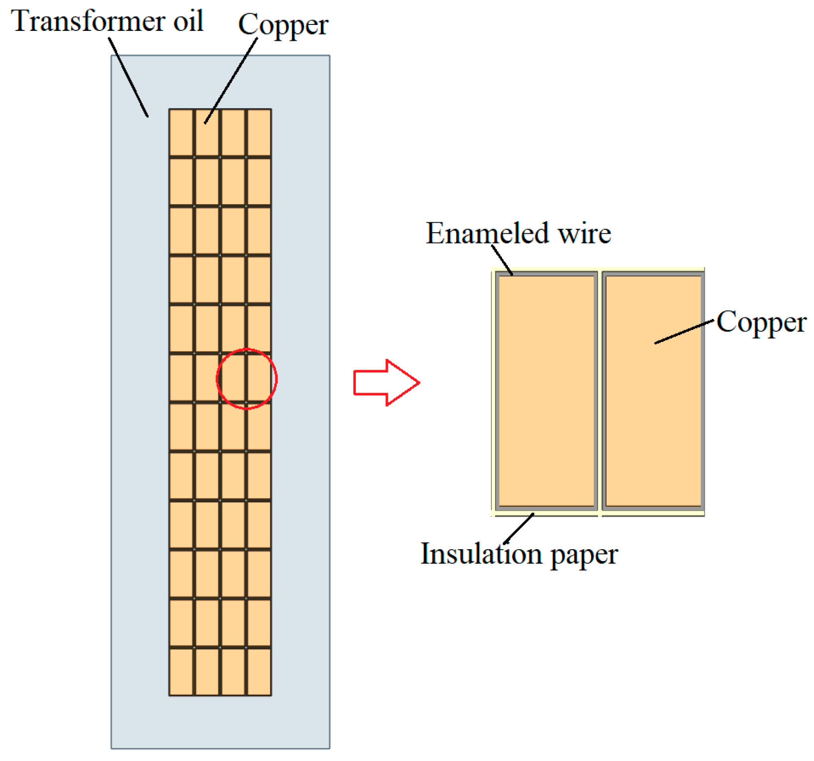
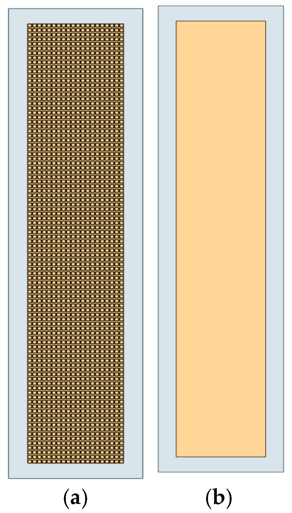
The model of low-voltage winding
The two-dimensional model of the low-voltage winding is shown in Figure 1, and the local model includes the winding, enameled wire, insulating paper, and transformer oil.
The low-voltage winding is a rectangular winding 8 mm × 4 mm long; the thickness of the winding is 0.15 mm, and the thickness of insulation paper is 0.2 mm. The number is 48.
B.
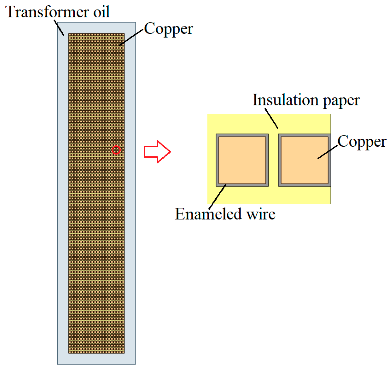
The model of high-voltage winding
The high-voltage winding of the amorphous alloy coil core transformer adopts layer winding, and the two-dimensional model of the high-voltage winding is shown in Figure 2. From the magnified partial view of high-voltage winding, it can be known that the high-voltage winding includes the winding, enameled wire, insulating paper and transformer oil. The high-voltage winding is 0.95 mm × 0.95 mm bar winding, the thickness of enameled wire is 0.11 mm, and the thickness of insulation paper is 0.2 mm. The number is 1920.
C.
Calculation method of equivalent thermal conductivity of winding
The equivalent model of high- and low-voltage windings is based on the principle of constant thermal resistance. The equivalent thermal conductivity is calculated by ensuring that the equivalent model is consistent with the fine model in thermal resistance.
The low-voltage winding is taken as an example to calculate the equivalent thermal conductivity. Since the main thermal conductivity direction of the low-voltage winding is axial thermal conductivity, the radial thermal conductivity has little influence on the winding temperature field distribution. Here, the axial thermal conductivity and radial thermal conductivity are considered equally to reduce the calculation time.
According to the principle of constant thermal resistance, when calculating the equivalent thermal conductivity of the axial winding, given the symmetry of the winding in the axial direction, we only need to analyze half of the winding structure, and the single row winding as shown in Figure 3. In the calculation, the axial length can be reduced to unit length (L = 1). In the subsequent analysis of nodes, nodes 1, 5, 9, 11, 13, 15, 17, and 18 represent insulating paper layers; nodes 2, 4, 6, 8, 10, 12, 14, and 16 represent enameled lines; and nodes 3 and 7 represent copper layers.
R = L λ S
According to the thermal resistance calculation Formula (1), where, L is the thermal conductivity distance, λ is the thermal conductivity coefficient, and S is the heating area.
Therefore, the calculation formula between the different nodes is given as follows.
The thermal resistance between node 1 and node 2 is as follows:
R 1 2 = L 1 2 λ insulation L y L + L 1 2 λ wire L y L
The thermal resistance between node 2 and node 3 is as follows:
R 2 3 = L 2 3 λ cu L y L + L 2 3 λ wire L y L
The thermal resistance between node 3 and node 4 is as follows:
R 3 4 = L 3 4 λ cu L y L + L 3 4 λ wire L y L
The thermal resistance between node 4 and node 5 is as follows:
R 4 5 = L 4 5 λ i n s u l a t i o n L y L + L 4 5 λ w i r e L y L
The thermal resistance between node 5 and node 6 is as follows:
R 5 6 = L 5 6 λ insulation L y L + L 5 6 λ wire L y L
The thermal resistance between node 6 and node 7 is as follows:
R 6 7 = L 6 7 λ cu L y L + L 6 7 λ wire L y L
The thermal resistance between node 7 and node 8 is as follows:
R 7 8 = L 7 8 λ cu L y L + L 7 8 λ wire L y L
Therefore, the total thermal resistance along the winding direction can be obtained by (9).
R cu = R 1 2 + R 2 3 + R 3 4 + R 4 5 + R 5 6 + R 6 7 + R 7 8
The total thermal conductivity is as follows:
G cu = 1 R cu
Similarly, the total thermal conductivities of the enameled line route and the insulated paper route are calculated.
G wire = 1 R wire
G insualtion = 1 R insulation
The total thermal conductivity according to the axial direction of the entire winding can be expressed by (13).
G = n 1 G insulation + n 2 G cu + n 3 G wire
The total thermal resistance is as follows:
R all = 1 G
The axial equivalent thermal conductivity is as follows:
λ eq = L xall R all L L yall
where λinsulation is the thermal conductivity of insulation paper, λwire is the thermal conductivity, λcu is the thermal conductivity of copper, Rall is the total thermal resistance, Gcu is the total thermal conductivity along the wire, Gwire is the total thermal conductivity along enameled wire, Ginsulation is the total thermal conductivity along insulation paper, n1 is the number of insulation papers between windings, n2 is the number of windings, n3 is the number of enameled wires, Lxall is the equivalent model axial length, and Lyall is the equivalent posterior radial length.

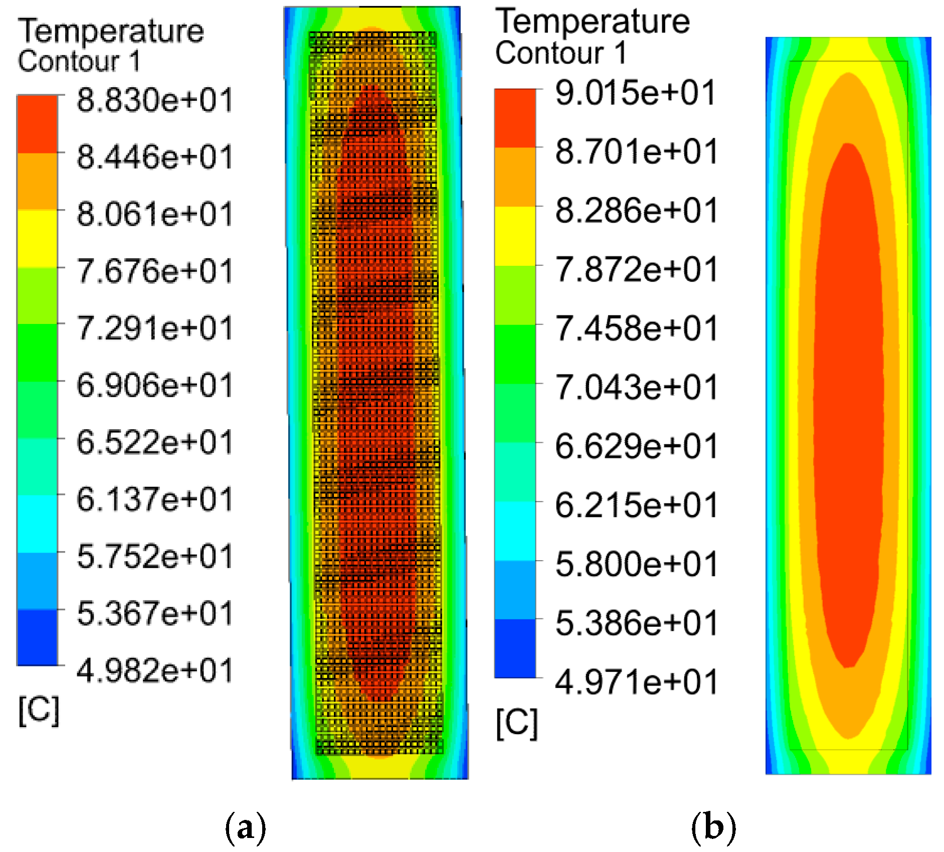
3. 2-D Simulation Validation

The refined model and equivalent model of low-voltage winding are shown in Figure 4, and the low-voltage winding is equivalent to a bulk conductor. The equivalent thermal conductivity is 0.61 W/(m·K), and the temperature distribution cloud map of the refined model is shown in Figure 5.
The refined model and equivalent model of the high-voltage winding of the amorphous alloy are established. As shown in Figure 6, the high-voltage winding is equivalent to a large conductor. By calculating the equivalent thermal conductivity, we can establish that the equivalent thermal conductivity of the high-voltage winding is 0.33 W/(m·K). And cloud maps of the temperature distribution of the refined model and equivalent post-temperature distribution are shown in Figure 7.
Considering the grid quantity in the 2D simulation model, both the refined model and equivalent model grids in this paper undergo encryption processing. The equivalent grid significantly reduces the number of grids while ensuring calculation accuracy. In grid processing, fine meshing of components is adopted, so the windings, insulation, and other parts of the refined model are precisely meshed to ensure the accuracy of the 2D refined simulation results. The different grid division diagrams are shown in Figure 8. The simulation results under different grid subdivisions are shown in Figure 9.
In the figure, from left to right, the grids are divided into three layers, ten layers, and twenty layers successively. It can be seen that as the number of grid layers increases, the simulation results hardly change. Therefore, this paper selects a 10-layer grid division, which is sufficient to meet the needs of the simulation.
According to the above simulation results, the highest temperature and average temperature of the low-voltage winding and high-voltage winding of the amorphous alloy coil core transformer are shown in Figure 10 and Figure 11.
According to simulation results, the maximum temperatures of the refined and equivalent models of the low-voltage winding are 113.7 °C and 112.6 °C, and the average temperatures are 111.4 °C and 109.1 °C. The maximum temperatures of the refined and equivalent models of the high-voltage winding are 88.3 °C and 90.15 °C, and the average temperatures are 84.5 °C and 85.2 °C. The maximum temperature error is controlled within 1.0%, and the average temperature error is controlled within 2.0%.
The reliability of the proposed method is verified by modifying different boundary conditions. Different heat dissipation coefficients were modified to obtain the highest and lowest temperatures of the refined and equivalent models as shown in Figure 12 and Figure 13. Therefore, under different heat dissipation coefficients, the equivalent thermal conductivity produced by this method still has the advantage of small error and high reliability.

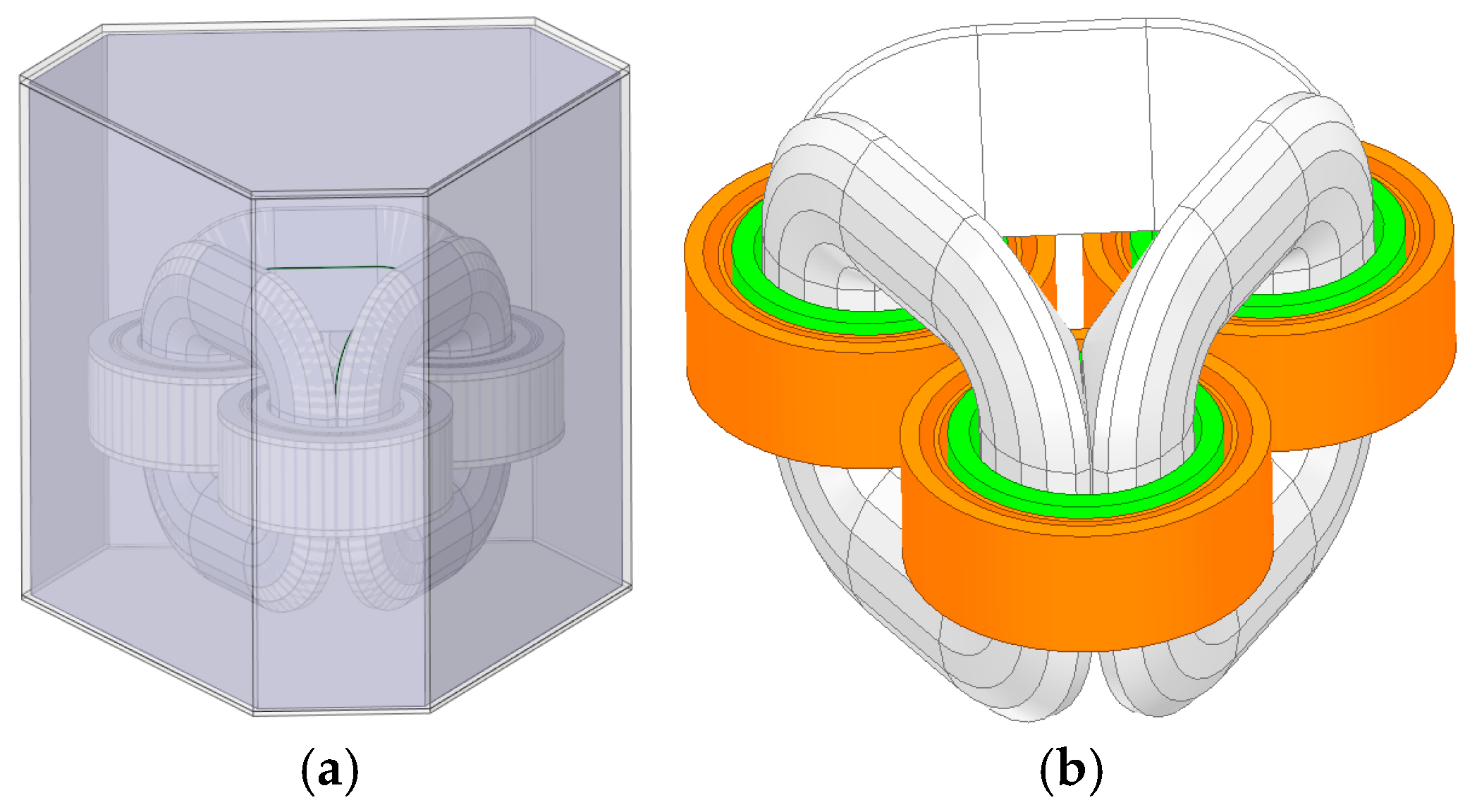
4. 3D Global Temperature Field Solution

A.
Temperature field modeling
The law of motion of fluid follows the law of conservation of physics, among which the most basic laws are the law of conservation of mass, the law of conservation of momentum, and the law of conservation of energy. In the turbulence condition, the system also satisfies the additional turbulence control equation.
The law of conservation of mass states that the increase in the mass of a body per unit time is equal to the net mass flowing into the microelement within the same time interval.
ρ t + · ( ρ u ) = 0
where ρ is heat flux, t is time, and u is velocity vector.
The law of conservation of momentum states that the time rate of change of fluid momentum within a microbody is equal to the sum of all forces acting on the microbody.
ρ u t + ρ u u = μ · u p x + S x ρ v t + ρ v u = μ · v p y + S y ρ w t + ρ w u = μ · w p z + S z
where ρ is voltage on the fluid microelement and μ is the dynamical viscosity.
The law of conservation of energy states that the time rate of change of energy within a microelement is equal to the net heat flow into the microelement plus the work done by volume forces and surface forces.
ρ T t + ρ u T = k c p · T + S T
where cp is the specific heat capacity, T is the thermodynamic temperature, k is the heat transfer coefficient of the fluid, and ST is the viscous dissipation term.
The turbulence control equation, namely, the turbulent k-ε equation, includes turbulent kinetic energy k equation and turbulent dissipation rate ε equation.
ρ k t + ρ u k = μ + μ t σ k · k ρ ε + μ t P G ρ ε t + ρ u ε = μ + μ t σ ε · ε ρ C 2 ε 2 k + μ t C 1 ε k P G P G = 2 u x 2 + v y 2 + w z 2 + u y + v x 2 + u z + w x 2 + v z + w y 2
where Cμ, σk, σε, C1, and C2 are constants.
The surface convection coefficient of the transformer frame is related to wind speed, and the relationship can be expressed as [21,22].
α 1 = α 0 ( 1 + γ ν ) T 0 25 3
where α0 is the convection coefficient of natural cooling, γ is air blowing efficiency coefficient, v is the speed of flowing air blowing stator frame, and T0 is the air temperature of stator frame. Among them, α0 is about 14, and γ is about 0.5.
In order to prepare for the construction of its geometric model and further calculation of its physical field boundary conditions, the main parameters are shown in Table 1.
The equivalent thermal conductivity is calculated by the above method, and the 3D model is established, as shown in Figure 14. The transformer cooling method is natural oil cooling, and there is no heat-dissipating rib on the outer wall of the tank.
  • B. Transformer loss
The main parameters of the transformer are shown in Table 2. Transformer loss is divided into no-load loss and load loss. No-load loss is mainly concentrated on the iron core, and the load loss is mainly winding loss and stray loss. In the simulation, when the heat source is loaded and the rated load is applied, the core loss is loaded according to the no-load loss, and the winding eddy current loss can be calculated according to the resistance loss and load loss minus stray loss. The main loss and loss density of the transformer are shown in Table 3.
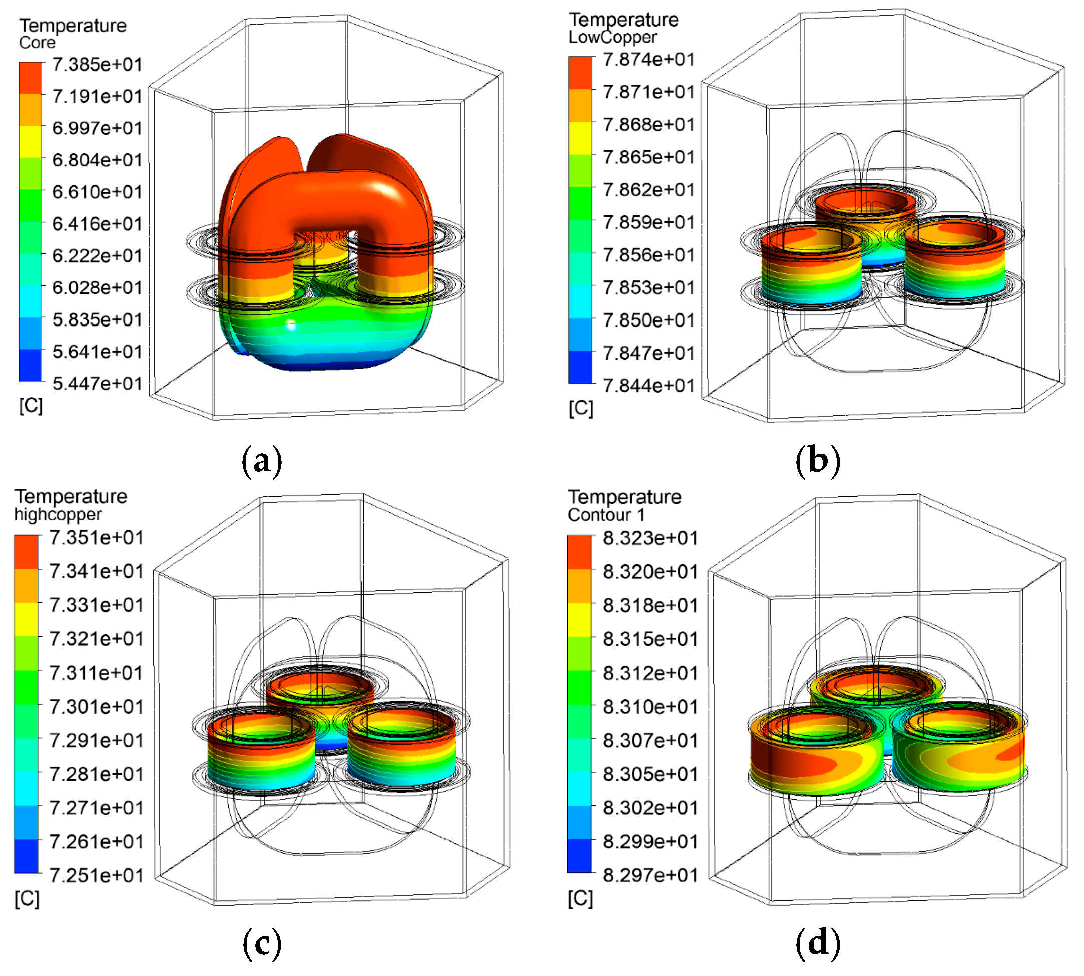
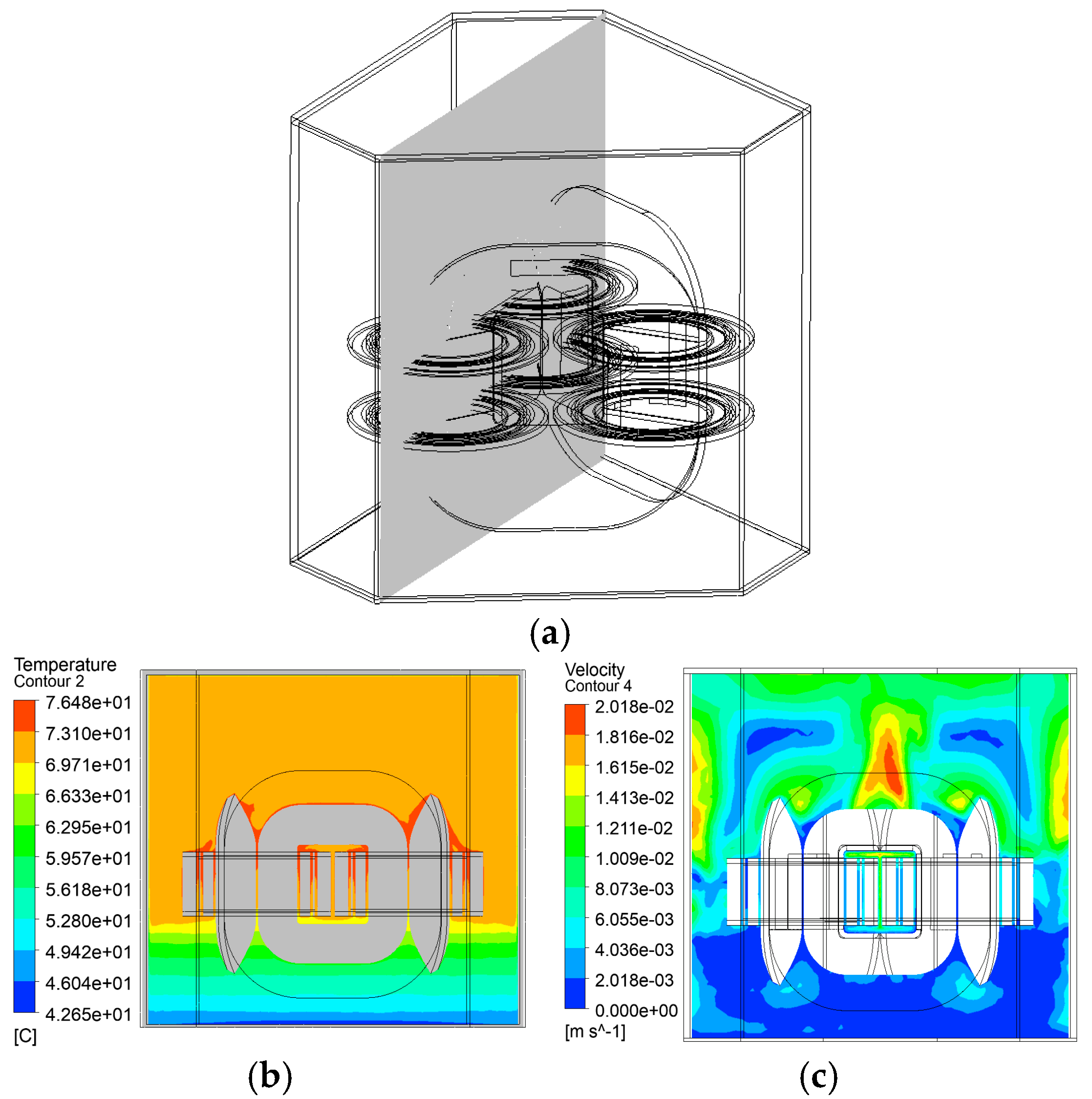
  • C. Temperature field simulation results
The thermal conductivity of the amorphous alloy is crucial in temperature field simulations [23,24]. And the thermal conductivity of amorphous alloys is selected as 20 W/(m·K).
The core and winding model, the single-phase winding model, and the finite element simulation are calculated to verify the reliability of the equivalent method. The finite element simulation results are shown in Figure 15. According to the analysis of the simulation results, the average temperature of the core is 55 K, and the temperature of the core is the lowest, about 54.5 °C. The high-voltage winding is divided into inner and outer layers; the maximum temperature values of the inner and outer high-voltage winding are 73.5 °C and 83.2 °C, respectively; the average temperature rises are 56.9 and 66.9 K, respectively; and the average temperature rise of the high-voltage winding is 60.9 K. The maximum temperature value of the low-voltage winding is 78.7 °C, and the average temperature rise of the low-voltage winding is 62.4 K.
In order to better observe the distribution characteristics of the temperature and flow rate of transformer oil, the cross section diagram is shown in Figure 14a, and the distribution characteristics of the temperature field and flow rate in this section are viewed, as shown in Figure 16b,c. The maximum temperature of transformer oil appears at the upper end of the oil passage between and the high- and low-voltage windings, and the maximum value is about 76.5 °C.

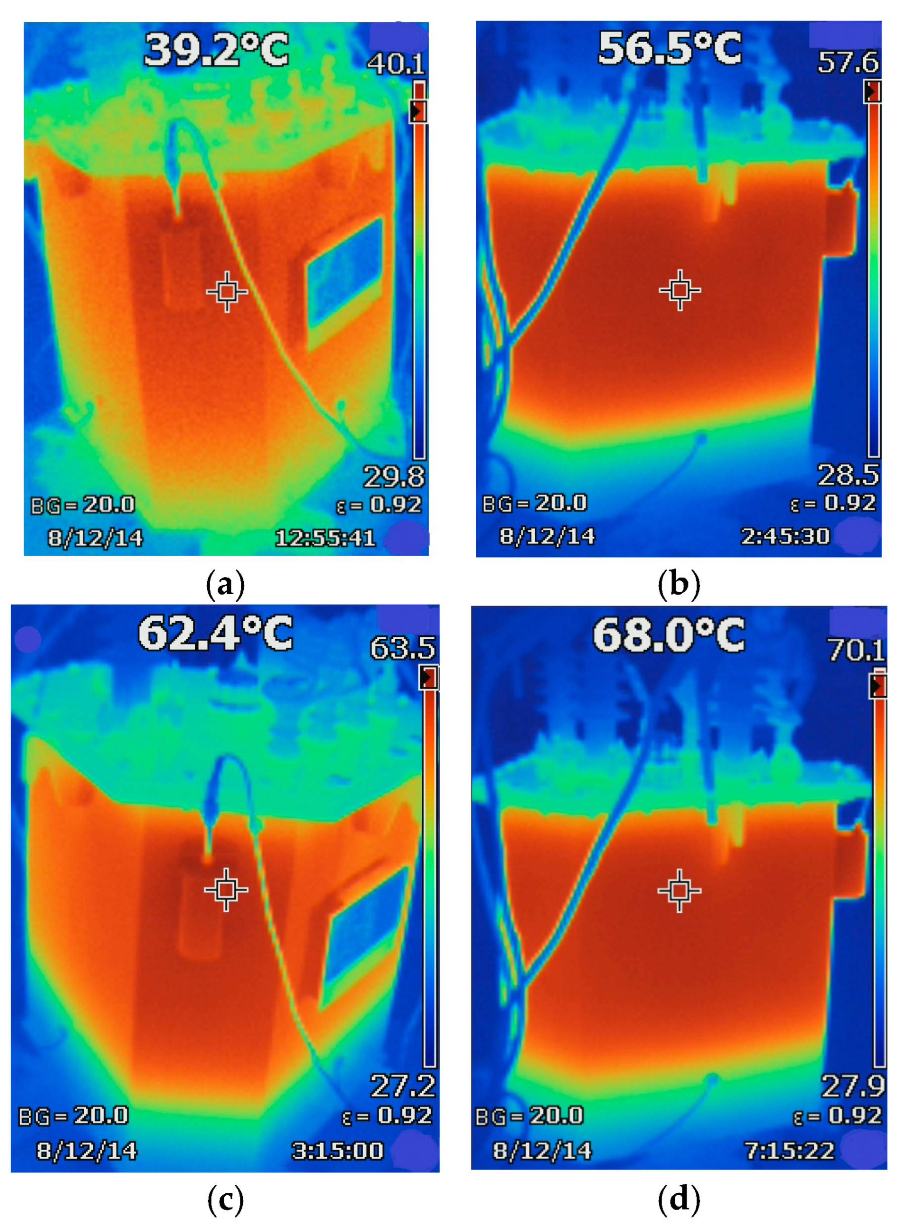
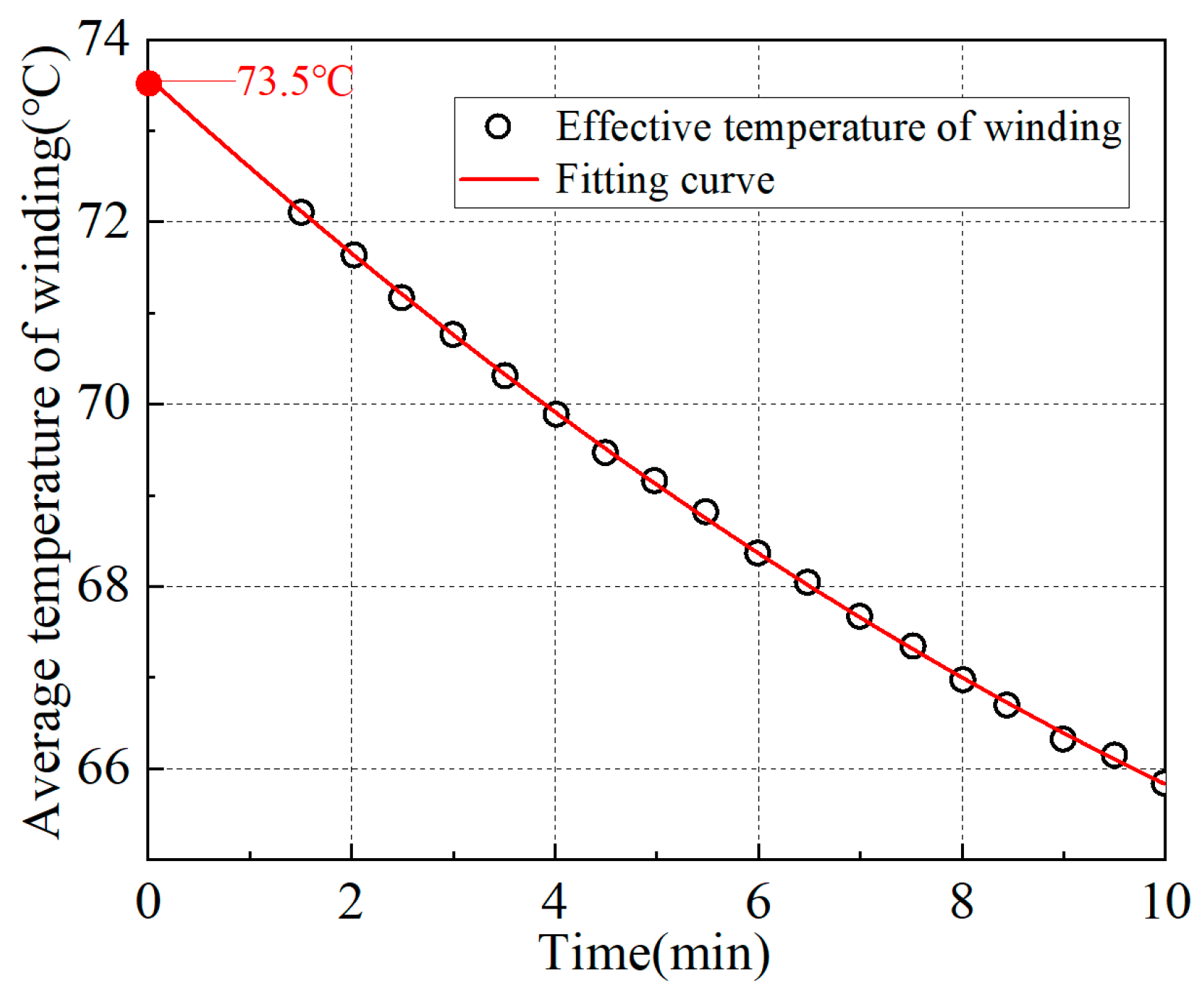
5. Experimental Measurement

The experimental platform was constructed with a rated capacity 50 KVA amorphous alloy 3D wound core transformer as the research object, as shown in Figure 17.
The accuracy and applicability of the equivalent method are verified by measuring the average temperature inside and outside the winding and transformer housing. The steady-state average temperature of the amorphous alloy transformers was measured by measuring the temperature curve at different times and the Fluke cloud diagram. As shown in Figure 18, the experimental 30 min Fluke mean temperature, 4 h Fluke, 8 h Fluke, and 12 h Fluke mean temperature clouds are presented, respectively.
Because of the measurement, the power is cut off and the sensor is connected, so for the high- and low-voltage windings, part of the heat will be dissipated, and the temperature will be calculated back through calculation. Therefore, the average temperature measurement of the high-voltage winding and low-voltage winding after the power supply is cut off as shown in Figure 19 and Figure 20.
The average temperature of the high- and low-voltage winding at the time point was calculated by curve fitting at 0 min based on the known detailed temperature data points. The results show that the average temperature is 73.2 °C, whereas the low-voltage winding is 73.5 °C.
Through experimental testing, the finite element simulation results and experimental test results obtained using this equivalent method are shown in Figure 21. From the finite element and experimental tests, the winding errors of both the low-voltage and the high-voltage winding are less than 3 K, which can verify the reliability of this method.

6. Conclusions

In order to accurately and quickly calculate the temperature rise distribution of the transformer, an equivalent modeling method for the temperature field of the transformer high-voltage winding is proposed. The proposed method is verified by finite element simulation analysis and experimental testing, and the following conclusions are obtained.
(1)
An equivalent modeling approach for the winding of amorphous alloy 3D wound core transformer is proposed. By homogenizing the high- and low-voltage windings into an equivalent bulk conductor, this method remarkably enhances the temperature field simulation speed while maintaining high calculation accuracy.
(2)
Based on the principle of unchanged equivalent thermal resistance, the influence of winding size parameters, arrangement characteristics, and other factors on the equivalent thermal conductivity is analyzed, and the equivalent thermal conductivities of and the high- and low-voltage windings are accurately obtained.
(3)
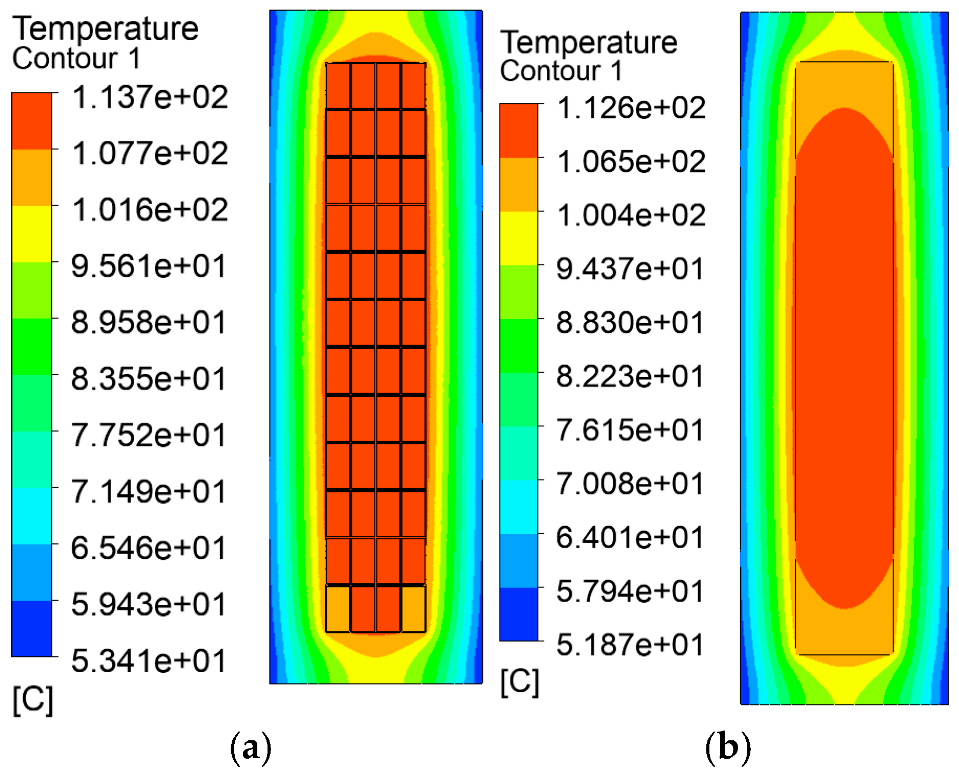
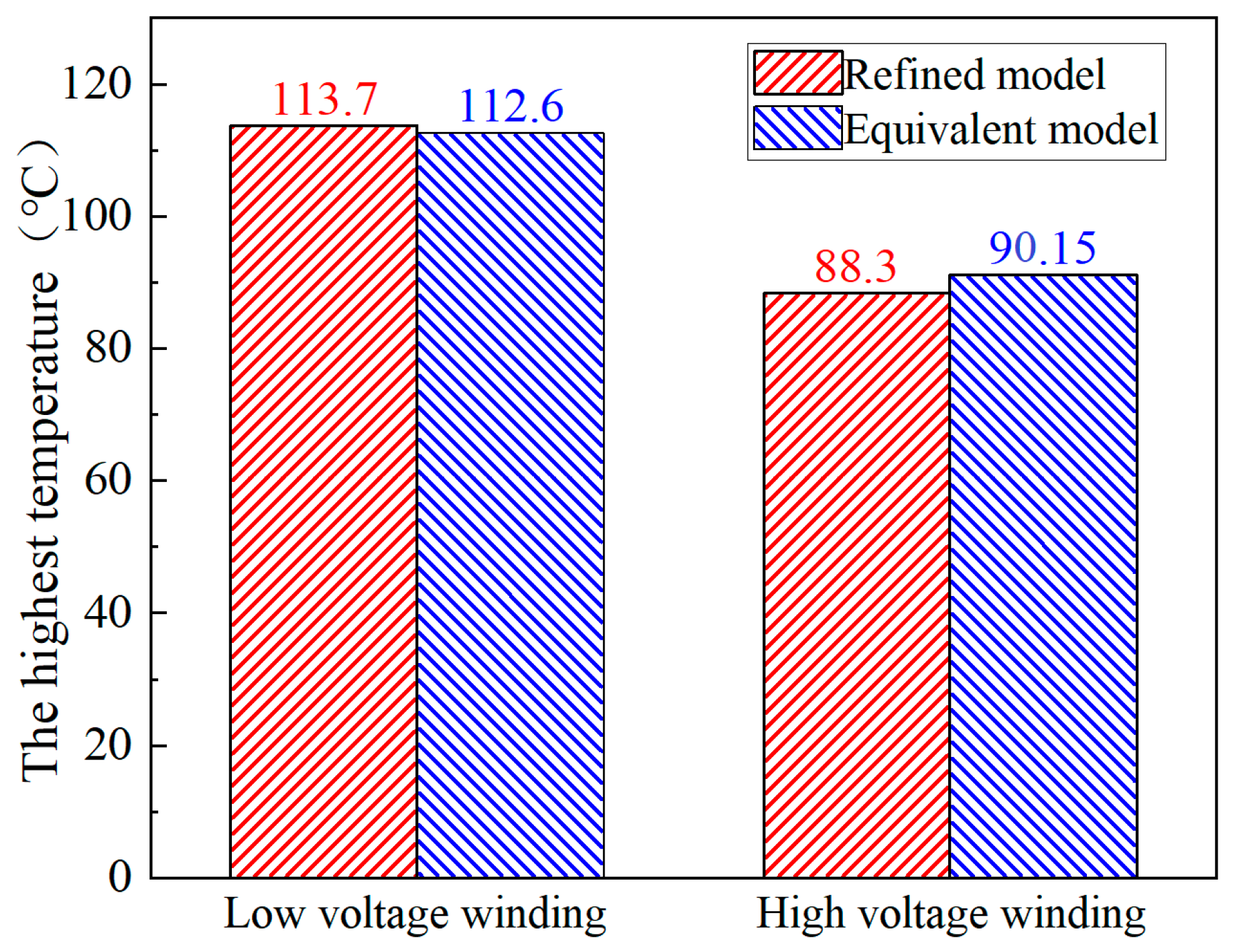
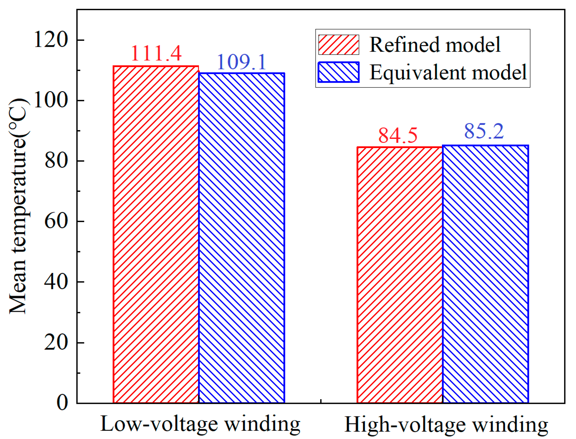
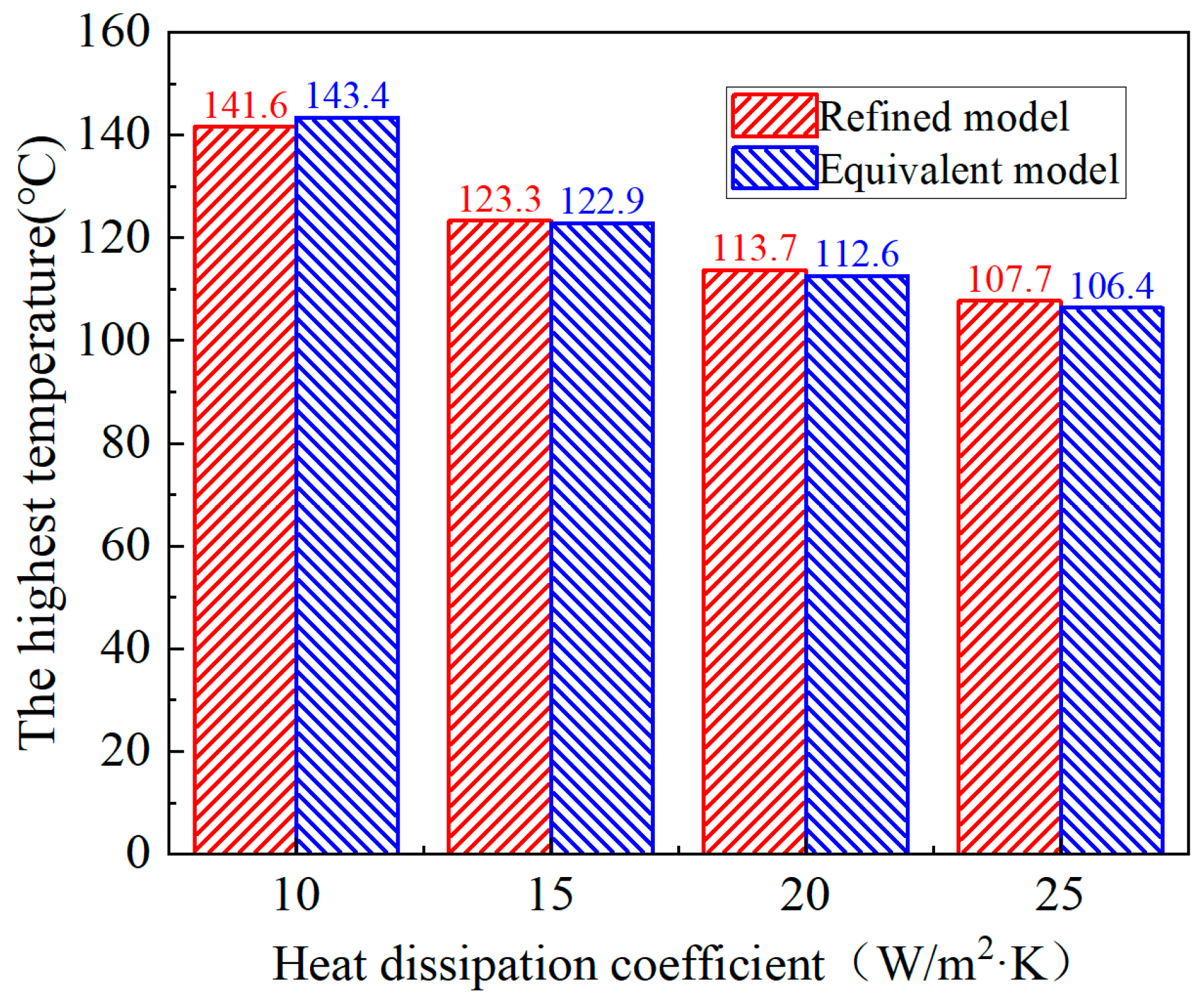
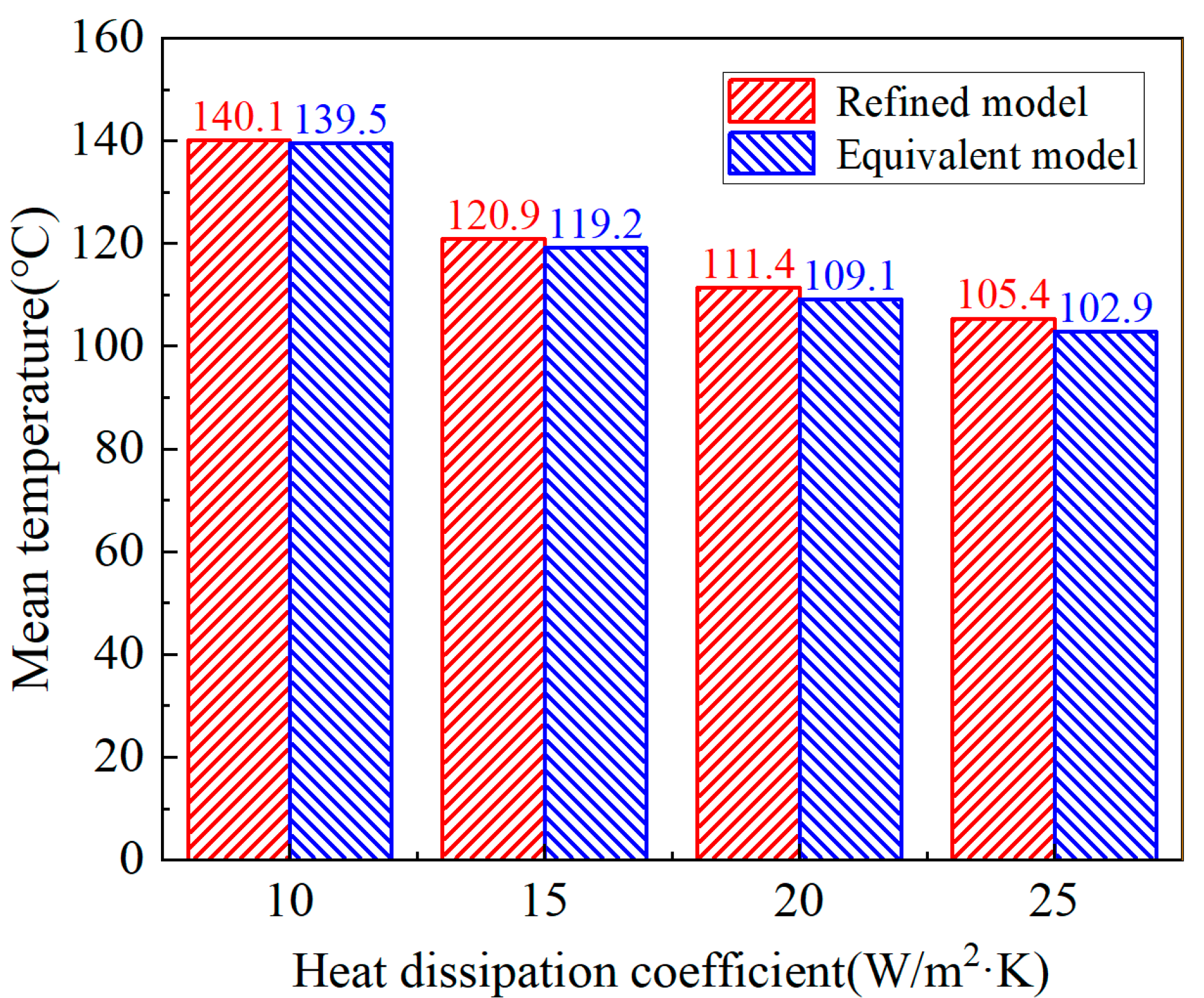
Through two-dimensional temperature field simulation analysis, it is shown that the maximum temperature and average temperature calculation errors of the equivalent model and the refined model are controlled within 1.0% and 2.0%, and the equivalent thermal conductivity still has high reliability under different boundary conditions.
(4)
The temperature field experiment tests the prototype, and the test results show that the error between high- and low-voltage winding simulation and experiment results is less than 3 K, which proves the effectiveness of this method in practical application.

Author Contributions

Software, J.H. and P.Z. (Peng Zhao); Validation, X.W.; Formal analysis, X.H. and Y.Y.; Investigation, X.Y.; Data curation, Z.D.; Writing—original draft, P.Z. (Pengzhe Zhuang); Writing—review & editing, Z.Y. All authors have read and agreed to the published version of the manuscript.

Funding

This research received no external funding.

Data Availability Statement

The original contributions presented in the study are included in the article, further inquiries can be directed to the corresponding author.

Conflicts of Interest

Authors Jianwei Han, Xiaolin Hou, Xinglong Yao, Zonghan Dai and Peng Zhao were employed by the Longyuan New Energy Co., Ltd. Authors Yunfei Yan and Xiaohui Wang were employed by the Xi’an Thermal Power Research Institute Co., Ltd. The remaining authors declare that the research was conducted in the absence of any commercial or financial relationships that could be construed as a potential conflict of interest.

References

  1. Li, Y.; Liu, N.; Liang, Y.; Xu, Y.-Y.; Lin, D.; Mu, H.-B.; Zhang, G.-J. A model of load capacity assessment for oil-immersed transformer by using temperature rise characteristics. Proc. CSEE 2018, 38, 6737–6746. [Google Scholar]
  2. Yuan, S.; Zhou, L.; Gou, X.; Zhu, Q.; Ding, S.; Wang, L.; Wang, D. Modeling method for thermal field of turbulent cooling dry-type on-board traction transformer in EMUs. IEEE Trans. Transp. Electrif. 2022, 8, 298–311. [Google Scholar] [CrossRef]
  3. Chen, Y.; Yang, Q.; Zhang, C.; Li, Y.; Li, X. Thermal network model of high-power dry-type transformer coupled with electromagnetic loss. IEEE Trans. Magn. 2022, 58, 1–5. [Google Scholar] [CrossRef]
  4. Niu, S.Y.; Yu, H.; Niu, S.X.; Jian, L. Power loss analysis and thermal assessment on wireless electric vehicle charging technology: The over-temperature risk of ground assembly needs attention. Appl. Energy 2020, 275, 115344. [Google Scholar] [CrossRef]
  5. Ortiz, C.; Skorek, A.W.; Lavoie, M.; Benard, P. Parallel CFD analysis of conjugate heat transfer in a dry-type transformer. IEEE Trans. Ind. Appl. 2009, 45, 1530–1534. [Google Scholar] [CrossRef]
  6. Niu, S.; Yu, H.; Jian, L. Thermal Behavior Analysis of Wireless Electric Vehicle Charging System under Various Misalignment Conditions. In Proceedings of the 2020 IEEE 4th Conference on Energy Internet and Energy System Integration (EI2), Wuhan, China, 30 October–1 November 2020; pp. 607–612. [Google Scholar]
  7. Zhao, Y.; Zhang, X.; Ho, S.L.; Fu, W.N. An adaptive mesh method in transient finite element analysis of magnetic field using a novel error estimator. IEEE Trans. Magn. 2012, 48, 4160–4163. [Google Scholar] [CrossRef]
  8. Gu, H.; Luo, Y.; Qiu, Y.; Hou, J. A fast solution method for large scale linear sparse equations based on parallelism. In Proceedings of the 2022 IEEE 5th International Conference on Electronics Technology (ICET), Chengdu, China, 13–16 May 2022; pp. 1337–1340. [Google Scholar]
  9. Liu, G.; Hu, W.; Hao, S.; Gao, C.; Liu, Y.; Wu, W.; Li, L. A fast computational method for internal temperature field in Oil-Immersed power transformers. Appl. Therm. Eng. 2024, 236, 121558. [Google Scholar] [CrossRef]
  10. Kiradjiev, K.B.; Halvorsen, S.A.; Van Gorder, R.A.; Howison, S.D. Maxwell-type models for the effective thermal conductivity of a porous material with radiative transfer in the voids. Int. J. Therm. Sci. 2019, 145, 106009. [Google Scholar] [CrossRef]
  11. Liu, X.; Gerada, D.; Xu, Z.; Corfield, M.; Gerada, C.; Yu, H. Effective thermal conductivity calculation and measurement of litz wire based on the porous metal materials structure. IEEE Trans. Ind. Electron. 2019, 67, 2667–2677. [Google Scholar] [CrossRef]
  12. Yi, X.; Yang, T.; Xiao, J.; Miljkovic, N.; King, W.P.; Haran, K.S. Equivalent thermal conductivity prediction of form-wound windings with litz wire including transposition effects. IEEE Trans. Ind. Appl. 2021, 57, 1440–1449. [Google Scholar] [CrossRef]
  13. Zhang, X.; Dong, T.; Zhou, F. Equivalent thermal conductivity estimation for compact electromagnetic windings. IEEE Trans. Ind. Electron. 2018, 66, 6210–6219. [Google Scholar] [CrossRef]
  14. Sun, Z.; Wang, Q.; Li, G.; Qian, Z.; Li, W.; Jing, J. A closed-form analytical method for reliable estimation of equivalent thermal conductivity of windings with round-profile conductors. IEEE Trans. Energy Convers. 2020, 36, 1143–1155. [Google Scholar] [CrossRef]
  15. Simpson, N.; Wrobel, R.; Mellor, P. Estimation of equivalent thermal parameters of impregnated electrical windings. IEEE Trans. Ind. Appl. 2013, 49, 2505–2515. [Google Scholar] [CrossRef]
  16. Deng, Q.; Wang, D.; Li, S.; Xie, F.; Zhao, J.; Liu, Z.; Liang, J.; Jiang, Y. Heat transfer performance of the solid microencapsulated fuel in light water reactors. Ann. Nucl. Energy 2022, 179, 109420. [Google Scholar] [CrossRef]
  17. Folsom, C.; Xing, C.; Jensen, C.; Ban, H.; Marshall, D.W. Experimental measurement and numerical modeling of the effective thermal conductivity of TRISO fuel compacts. J. Nucl. Mater. 2015, 458, 198–205. [Google Scholar] [CrossRef]
  18. Wang, J.; Wang, M.; Li, Z. A lattice Boltzmann algorithm for fluid–solid conjugate heat transfer. Int. J. Therm. Sci. 2007, 46, 228–234. [Google Scholar] [CrossRef]
  19. Yang, Y.; Fathidoost, M.; Oyedeji, T.D.; Bondi, P.; Zhou, X.; Egger, H.; Xu, B.-X. A diffuse-interface model of anisotropic interface thermal conductivity and its application in thermal homogenization of composites. Scripta Mater. 2022, 212, 114537. [Google Scholar] [CrossRef]
  20. Pitchai, P.; Guruprasad, P.J. Determination of the influence of interfacial thermal resistance in a three phase composite using variational asymptotic based homogenization method. Int. J. Heat Mass Transfer 2020, 155, 119889. [Google Scholar] [CrossRef]
  21. Staton, D.; Boglietti, A.; Cavagnino, A. Solving the more difficult aspects of electric motor thermal analysis in small and medium size industrial induction motors. IEEE Trans. Energy Convers. 2005, 20, 620–628. [Google Scholar] [CrossRef]
  22. Ahmed, F.; Kar, N.C. Analysis of end-winding thermal effects in a totally enclosed fan-cooled induction motor with a die cast copper rotor. IEEE Trans. Ind. Appl. 2017, 53, 3098–3109. [Google Scholar] [CrossRef]
  23. Kwon, S.; Zheng, J.L.; Wingert, M.C.; Cui, S.; Chen, R.K. Unusually High and Anisotropic Thermal Conductivity in Amorphous Silicon Nanostructures. ACS Nano 2017, 11, 2470–2476. [Google Scholar] [CrossRef] [PubMed]
  24. Ishibe, T.; Okuhata, R.; Kaneko, T.; Yoshiya, M.; Nakashima, S.; Ishida, A.; Nakamura, Y. Heat transport through propagon-phonon interaction in epitaxial amorphous-crystalline multilayers. Commun. Phys. 2021, 4, 153. [Google Scholar] [CrossRef]
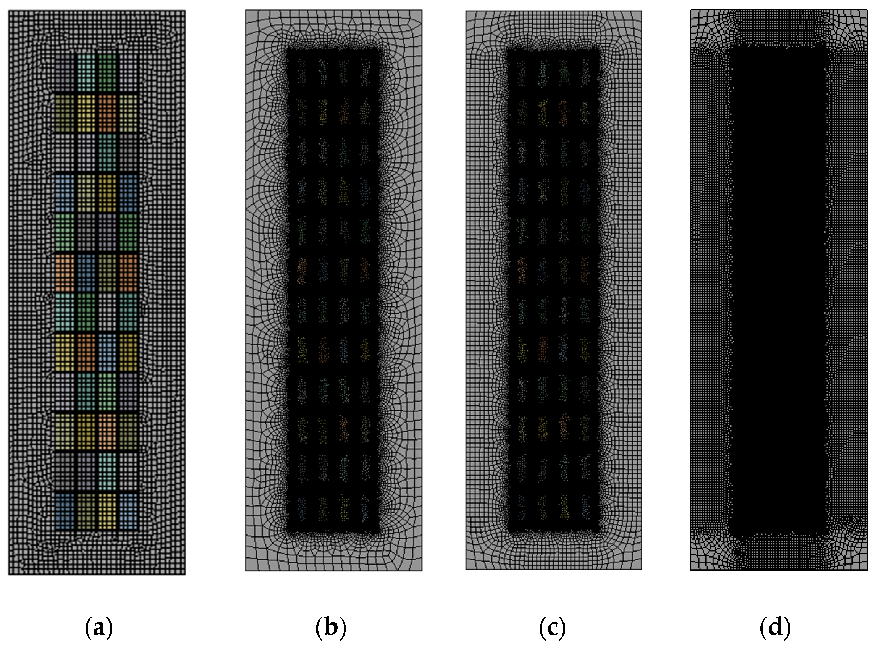
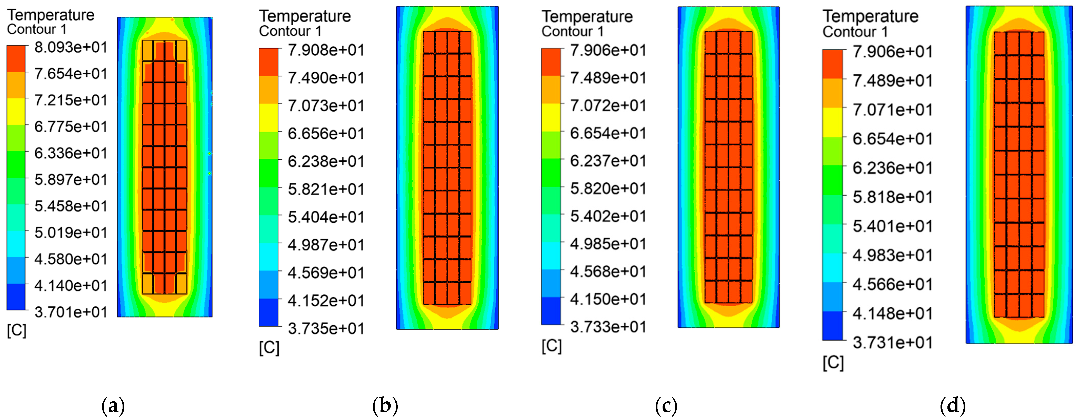
Figure 1. Schematic diagram of low-voltage winding of transformer.
Energies 18 03212 g001
Figure 2. Schematic diagram of high-voltage winding of transformer.
Energies 18 03212 g002
Figure 3. Heat resistance distribution of the single-row winding group.
Energies 18 03212 g003
Figure 4. 2D winding diagram for low-voltage winding. (a) Refined model. (b) Equivalent model.
Energies 18 03212 g004
Figure 5. Temperature field distribution before and after equivalent low-voltage winding of amorphous alloy transformer. (a) Refined model. (b) Equivalent model.
Energies 18 03212 g005
Figure 6. 2D winding diagram for high-voltage winding. (a) Refined model. (b) Equivalent model.
Energies 18 03212 g006
Figure 7. Temperature field distribution before and after equivalent high-voltage winding of amorphous alloy transformer. (a) Refined model. (b) Equivalent model.
Energies 18 03212 g007
Figure 8. Different grid division diagrams. (a) Default split grid. (b) 3-layer grid. (c) 10-layer grid. (d) 20-layer grid.
Energies 18 03212 g008
Figure 9. Simulation results under different grid subdivisions. (a) Default split grid. (b) 3-layer grid. (c) 10-layer grid. (d) 20-layer grid.
Energies 18 03212 g009
Figure 10. Maximum temperature distribution map of the refined and equivalent models.
Energies 18 03212 g010
Figure 11. Average temperature distribution map of the refined and equivalent models.
Energies 18 03212 g011
Figure 12. Maximum temperature for different cooling conditions.
Energies 18 03212 g012
Figure 13. Average temperature of the different heat dissipation conditions.
Energies 18 03212 g013
Figure 14. Three-dimensional temperature field solving model. (a) Whole solution region. (b) Iron core and its winding model.
Energies 18 03212 g014
Figure 15. Calculation results of the temperature field simulation. (a) Iron core. (b) Low-voltage winding. (c) Internal high-voltage winding. (d) Outer high-voltage winding.
Energies 18 03212 g015
Figure 16. Results for the oil of cross section. (a) Cross section diagram. (b) Velocity distribution. (c) Temperature distribution.
Energies 18 03212 g016
Figure 17. Experimental test. (a) Test platform. (b) Thermal image.
Energies 18 03212 g017
Figure 18. Temperature distribution tested by infrared thermal imager. (a) Cloud plot of the experimental temperature at 30 min. (b) Cloud plot of the experimental temperature at 4 h. (c) Cloud plot of the experimental temperature at 8 h. (d) Cloud plot of the experimental temperature at 12 h.
Energies 18 03212 g018
Figure 19. Average temperature change curve of high-voltage winding after power cut off.
Energies 18 03212 g019
Figure 20. Average temperature change curve of low-voltage winding after power cut off.
Energies 18 03212 g020
Figure 21. Comparison of finite element simulation and experimental test results diagram.
Energies 18 03212 g021
Table 1. The number of grids under different grid subdivisions and the calculated temperature.
Case The Number of GridsMeasure (°C)
1Default split grid32,35480.93
23-layer grid218,47879.08
310-layer grid220,95279.06
420-layer grid235,63479.06
Table 2. 50 kVA transformer.
ParameterValue
Rated voltage/kV10 × (1 ± 5%)/0.4
Capacity/kVA50
Connection modeDynl1
Core radius/mm80.0
Number of turns49
Low-voltage winding height/mm109
High-voltage winding height/mm104
Low-voltage winding radius/mm208/173
High-voltage winding radius/mm288/218
Short-circuit impedance/%4.0
Table 3. Transformer loss loading value.
ParameterHigh-Voltage WindingLow-Voltage WindingCore
Loss/W396.3310.840
Volume/m30.00440.00310.0276
Loss density (W/m3)89,923.1100,045.11449.3
Disclaimer/Publisher’s Note: The statements, opinions and data contained in all publications are solely those of the individual author(s) and contributor(s) and not of MDPI and/or the editor(s). MDPI and/or the editor(s) disclaim responsibility for any injury to people or property resulting from any ideas, methods, instructions or products referred to in the content.

