Modeling of Battery Storage of Photovoltaic Power Plants Using Machine Learning Methods

Abstract

The massive integration of variable renewable energy sources (RESs) poses the gradual necessity for new power system architectures with wide implementation of distributed battery energy storage systems (BESSs), which support power system stability, energy management, and control. This research presents a methodology and realization of a set of 11 BESS models based on different machine learning methods. The performance of the proposed models is tested using real-life BESS data, after which a comparative evaluation is presented. Based on the results achieved, a valuable discussion and conclusions about the models’ performance are made. This study compares the results of feedforward neural networks (FNNs), a homogeneous ensemble of FNNs, multiple linear regression, multiple linear regression with polynomial features, decision-tree-based models like XGBoost, CatBoost, and LightGBM, and heterogeneous ensembles of decision tree modes in the day-ahead forecasting of an existing real-life BESS in a PV power plant. A Bayesian hyperparameter search is proposed and implemented for all of the included models. Among the main objectives of this study is to propose hyperparameter optimization for the included models, research the optimal training period for the available data, and find the best model from the ones included in the study. Additional objectives are to compare the test results of heterogeneous and homogeneous ensembles, and grid search vs. Bayesian hyperparameter optimizations. Also, as part of the deep learning FNN analysis study, a customized early stopping function is introduced. The results show that the heterogeneous ensemble model with three decision trees and linear regression as main model achieves the highest average R² of 0.792 and the second-best nRMSE of 0.669% using a 30-day training period. CatBoost provides the best results, with an nRMSE of 0.662% for a 30-day training period, and offers competitive results for R²—0.772. This study underscores the significance of model selection and training period optimization for improving battery performance forecasting in energy management systems. The trained models or pipelines in this study could potentially serve as a foundation for transfer learning in future studies.

1. Introduction

The proactive policy incentives of the EU combined with the improved technological and economic competitiveness made the photovoltaic (PV) power plants the fastest growing and most competitive carbon-free source of electricity [1].

Renewable PV and wind generators tend to gradually increase their share and are expected to dominate the electricity generation mix in the near future [2].

Despite their advantages, renewable energy sources (RESs) are characterized by significant inherent volatility, and unlike conventional generators, their implementation presents various functional, planning, operational, and control challenges that need to be considered [3,4].

One way to respond to these challenges is to implement new electricity market schemes and structures that will smartly change our life and behavior towards increasing consumption (demand) flexibility in order to adapt as much as possible to the generation presence and fluctuations [5,6,7,8].

Not excluding the above, the smart BESS implementation in stationary storage devices and/or electric vehicles represents one of the most widely applicable and scalable solutions. In addition to power and energy balancing, the BESS with grid-forming and grid-supporting inverters play vital roles in maintaining the angle, voltage, frequency, and new forms of converter-driven power system stability [9,10].

Modeling battery storage and understanding BESS performance is of key importance for future power systems. Adequate modeling provides significant support for the improved implementation of BESSs while assisting the design, exploitation, and prediction of PV power plants with BESSs.

Due to the great variance of BESSs and PV power plant equipment types, topologies, and architectures, the artificial intelligence methods offer many advantages over other types of models by representing a very practical approach for modeling and simulation without getting into detailed and hard-to-find internal properties of the evaluated systems.

A key motivation of this research is the need to improve the forecasting accuracy of battery energy storage systems (BESSs) integrated with photovoltaics (PVs), which is an essential part of effective renewable energy management. This study addresses a gap in the existing literature where traditional forecasting methods often suffer from data drift and suboptimal training periods, resulting in reduced accuracy. This paper aims to present a comprehensive comparison of multiple linear regression (MR), MR with polynomial features (PFs), advanced neural networks (FNNs), ensemble FNN, XGBoost, CatBoost, LightGBM, and ensembles of decision tree models in the task of the day-ahead forecasting of real-life battery energy storage systems, which is a part of the PV power plant. The abovementioned algorithms are included in this research due to their suitability for regression tasks. This study features an optimized training period search for the included models and data. It applies Bayesian hyperparameter search to refine the model hyperparameters and evaluates the performance of the models using various metrics, providing a detailed analysis of their performance. This approach differs from previous works on this topic by providing a systematic method to optimize and compare different forecasting models, which can potentially improve the accuracy and efficiency of BESS trend forecasting in real-world applications. By implementing the homogeneous FNN ensemble model and heterogeneous DT models, this research compares the test results and checks if the metrics of the single models have been improved. Also, it compares the forecast results, achieved via grid search and Bayesian hyperparameter optimizations, for the same models. Additionally, this study proposes an early stop recall, adapted for FNNs, to avoid overfitting, thus improving the reliability of the model.

Many studies compare various machine learning methods [11]. Machine learning methods are increasingly applied in more and more areas regarding energy storage devices, specifically including BESSs as well. In [12,13,14,15], the main ML methods and their application in battery storage simulations for the calculation of SOC, SOH, battery lifetime estimation and prediction, battery fault diagnosis, degradation analysis, battery design and optimization, battery modeling, behavior prediction, and voltage prediction are presented.

Still, it is of prior interest to implement a study on the typical charge/discharge operation cycles of battery energy storage connected to a real photovoltaic power plant, load, and AC generation source. In such real-life conditions, the battery capacity, power, and voltage depend on different ambient parameters—such as battery temperature, solar radiation, AC load, and generation power.

Various [16] ensemble methods of ML and DL models have recently been increasingly implemented in the area of the prediction of the energy generation of PV power plants with and without BESSs [17,18,19].

The studied hyperparameters in this study for the MR are “with” and “without polynomial features” and optimal feature degrees, both with and without feature interaction. The studied hyperparameters of the FNNs are learning rate, number of neuron layers, number of neurons, and activation function, and the list could be extended. A customized early stopping callback function for the FNNs is proposed. The function stops the FNN model training (after waiting a preset number of epochs) if the training cannot provide a more accurate model. The proposed function observes two metrics cratering and remains open, providing the ability to add more. An ensemble of FNNs is generated, based on the results of the hyperparameter search and the given number of FNNs, trained with the proposed customized early stopping callback. The hyperparameters studied for the XGBoost model are max depth, learning rate, n_estimators, min_child_weight, gamma, subsample, colsample bytree, reg_alpha, and reg_lambda. The studied hyperparameters for the CatBoost model are learning rate, depth, subsample, colsample bylevel, and min_data_in_leaf. The studied hyperparameters for the LightGBM model are learning rate, n_leaves, subsample, colsample_bytree, and min_data_in_leaf. Four heterogeneous ensembles of decision trees models, with the base models of XGBoost, CatBoost and LightGBM models and their optimized hyperparameters, and four different main models—XGBoost, CatBoost, LightGBM and linear regression—are generated. The types and values of the hyperparameters of the base models are chosen. The hyperparameters of each main model of the DT ensembles are the same as for the single models, and their values are additionally optimized for each model.

Finally, a comparison between FNNs, the ensemble of FNNs, MR, poly-MR, XGBoost, CatBoost, LightGBM and the four ensembles of the decision tree models is proposed.

The remainder of this article is structured as follows: First, in Section 2, a literature review of common research problems is presented. In Section 3, the methods used are described. Section 4 describes the test system and data used for method implementation. Section 5 provides the data description and pre-processing. Section 6 describes the training process. Section 7 presents the results and analysis. Section 8 offers a discussion, and Section 9 offers conclusions from the study.

2. Literature Review

In [20], modeling of the SOC and voltage of a lithium-ion battery is proposed, based on the feedforward neural network and nonlinear autoregressive exogenous model (time series), respectively. The paper shows the modeling and training data, and the achieved error regarding the voltage is 4%. The authors mention that some error peak could be noticed after each discharge due to the high degree of battery discharge. The input parameters of the model are the current, battery temperature, and SOC of the battery.

A laboratory LiFePO4 battery model using predefined charge and discharge cycles is presented in [21]. The model uses 10 neurons in the hidden layer, with a total weight of 71. The metrics used are MSE and nRMSE. The best model, based on conjugate gradient backpropagation with Fletcher–Reeves restarts, achieved an MSE of 0.0002 and an nRMSE equal to 0.8437. The way the nRMSE was initialized means that it can vary between −∞ (no fit) and 1 (perfect fit).

In reality, many applications with battery energy storage include photovoltaic power plants, inverters, electrical loads, and AC generation on the inverter input (which might be an electrical network or a hydro or diesel generator). If the BESS model is prepared, trained, and tested in laboratory conditions, then its structure, capacity (number of coefficients), and complexity will be designed and calculated to match the laboratory testing scheme and conditions. In real-life situations, the model must be able to take into account many more physical characteristics and interconnections of different types of electrical equipment [22,23].

In [24], a model for predicting the voltage of lead–acid batteries, utilizing convolutional neural networks (CNNs) and multi-layer perceptrons (MLPs) is presented. The overarching aim of the study is to forecast battery lifetime by establishing a voltage decay model.

In [25], a research endeavor proposes a study centered on ensemble learning with the V-IOWGA operator, a method involving time-varying weight allocation, to predict battery capacity across cycles. The study employs various machine learning techniques including the radial basis function (RBF), support vector regression (SVR), and autoregressive integrated moving average (ARIMA). An operator is utilized to aggregate predictions from base models within the ensemble. While conventional studies often utilize time-invariant trained weights, the introduction of a time-dependent weight allocation operator could prove to be beneficial in scenarios where prediction results are influenced by specific time points.

In [26], an investigation introduces a method for creating and evaluating an automated ensemble model with automatically generated and selected architectures, including the determination of the number of base models, layers, and nodes. The study also incorporates negative correlation learning for training neural networks (NNs). This automated approach is validated across diverse classification tasks, offering streamlined training procedures. In the context of single-type regression tasks, this approach could potentially replace traditional grid search methods with hyperparameter optimization during training.

In [27], a comprehensive study undertakes a review and comparative analysis of various neural network (NN) methods for predicting battery state. These methods include the extreme learning machine, deep convolutional NN, deep NN, recurrent NN, DCNN with ensemble transfer learning, adaptive long short-term memory (LSTM), gated recurrent unit, and Gaussian process regression, among others.

In [28], researchers propose a study focusing on model-based extreme learning machine techniques, aiming to enhance long-term prediction capabilities by substituting activation functions with a set of models. The model is designed to predict battery voltage, temperature, and power.

In [29], a study conducts a thorough comparison of different deep learning (DL) methods for predicting the state of health (SOH) and state of charge (SOC) of batteries, including long short-term memory recurrent neural networks (LSTM-RNNs), convolutional neural networks (CNNs), deep neural networks (DNNs), and other approaches.

While many of those works show good results and extensive research with different neural networks, it is difficult to notice a comparison between DL and ML methods, and especially multiple linear regression with polynomial features.

For example, work [30] proposes research on the optimal ML method. This research shows that on the presented data, multiple linear regression with polynomial features provides better results compared with the other ML methods used —multiple linear regression, lasso regression, ridge regression, decision trees, and random forest. The study shows that achieving relatively high accuracy is possible even with only two main independent parameters. Additionally, it is found that using shorter training periods could provide much better results than using longer training periods, mainly due to data drift.

Study [31] provides a comprehensive review of the use of artificial neural networks (ANNs) in estimating various states of Li-ion batteries, including state of charge, state of health, remaining useful life, thermal state, and other parameters. The estimation accuracy and robustness are analyzed using error evaluation metrics and study remarks. It is noted that Feedforward Neural Networks were the most commonly used for estimating Li-ion battery states. Additionally, Convolutional Neural Networks have shown good estimation performance in several studies and demonstrate significant potential.

Paper [32] proposes a novel SOC estimation method for lithium-ion energy storage systems using an LSTM-CNN driven by actual operating data from a photovoltaic energy storage system. This approach avoids traditional artificial battery models and addresses estimation deviations caused by voltage jumps. The method achieves accurate SOC estimation with an RMSE less than 0.31% over a full day of operation.

In addition, paper [33] reviews machine-learning-based SOC estimation methods for lithium-ion batteries, focusing on data collection and preparation, model selection and training, and model evaluation and optimization. It provides a thorough analysis to lower the research barrier and advance intelligent SOC estimation in the battery field.

Work [34] presents a closed-loop SOC estimation method for lithium-ion batteries using a simulated annealing-optimized support vector regression (SA-SVR) combined with a minimum-error-entropy-based extended Kalman filter (MEE-EKF). This approach enhances estimation accuracy and generalization by optimizing SVR parameters and processing through the MEE-EKF. Validated under various operating conditions, the method achieves a mean absolute error below 0.60% and a root mean square error below 0.73%.

In [35], a generally applicable stacked ensemble algorithm (deep stacked ensemble of XGBoost) is proposed utilizing two deep learning algorithms, namely artificial neural network (ANN) and long short-term memory (LSTM) as base models for solar energy forecast.

In [36], a hybrid model is presented and compared with six benchmark methods based on CatBoost, KNN, DT, SVR, XGBoost, and LGBM in different seasons and forecasting horizons.

On top of the above, in recent years, a growing number of studies have focused on integrating physical laws into neural network architectures, resulting in a hybrid modeling paradigm known as physics-informed neural networks (PINNs). These models aim to combine the robustness and interpretability of physics-based formulations with the flexibility and predictive accuracy of data-driven methods. This hybrid approach has been increasingly applied across various domains of battery modeling and state of health (SOH) estimation, addressing longstanding issues such as generalizability, data scarcity, and physical inconsistency in predictions.

In [37], Wang et al. proposed a PINN framework for SOH estimation that integrates empirical degradation models with state–space equations. By extracting statistical features from pre-charging data, the model is capable of generalizing across various battery chemistries and cycling conditions. Their method demonstrated superior performance on multiple datasets, achieving a mean absolute percentage error (MAPE) of 0.87% and showcasing remarkable robustness in small-sample and transfer-learning scenarios.

Luo et al. in [38] introduced a hybrid PINN (PIHNN) framework that incorporates a comprehensive electrochemical–thermal–mechanical–side reaction (ETMS) aging model into a neural network structure. Their work emphasizes the monotonic relationship between membrane resistance and capacity degradation as a physical constraint embedded within the network’s loss function. The model, enhanced through Bayesian optimization for hyperparameter tuning, outperforms traditional data-driven methods in predictive accuracy and computational efficiency under varying charge/discharge rates.

In another effort to enhance interpretability and parameter fidelity, Wang et al. in [39] developed a PINN approach specifically designed for identifying parameters within electrochemical models (EMs). Their strategy involves categorizing parameters based on discharge profiles and integrating domain-specific physical laws directly into the training process. This results in the high-fidelity estimation of electrochemical parameters, even for batteries with unknown properties, thus improving the practical applicability of EMs for real-time diagnostics.

Beyond the specific context of lithium-ion batteries, Hu et al. in [40] provided a comprehensive overview of the numerical frameworks and applications of PINNs within computational solid mechanics. Their review highlights the value of PINNs in addressing inverse problems, incorporating boundary conditions and physical priors, and solving complex high-dimensional partial differential equations (PDEs). This general-purpose framework underlines the cross-domain versatility and foundational strength of PINNs as a surrogate modeling tool in scientific computing.

Farea et al. in [41] offered a broad survey of PINN methodologies, detailing the various integration techniques of physical constraints into neural architectures and their application to both forward and inverse problems across physics and engineering domains. Their work provides a foundational understanding of PINNs, illustrating how the approach can address issues related to data scarcity, model generalization, and physical inconsistency, thereby paving the way for future interdisciplinary applications.

In [42], a study proposes a hybrid model integrating physics-based aging-aware modeling with feedforward neural networks (FNNs). The calculated physical parameters derived from the physical model are integrated as input information for the FNN. Moreover, the physical model is structured as a modular block, enabling the construction of various physics-based models tailored for specific modeling tasks and objects.

While the reviewed literature demonstrates the wide application of machine learning and deep learning models for battery state prediction, most studies either focus on idealized laboratory conditions or narrow use cases (e.g., single-battery chemistries or state estimation). There is a lack of comparative studies evaluating both simple and complex ML models—such as Multiple Linear Regression, gradient boosting, and Feedforward Neural Networks—on real-world photovoltaic battery system data, particularly for direct voltage forecasting. This study addresses that gap by systematically comparing such models across different training periods, aiming to support practical deployment in PV battery applications.

3. Methodology

The main methods used in this research include multiple linear regression, both with and without polynomial features, feedforward neural networks (FNNs), stacked ensemble models with homogeneous FNNs, with FNN as the primary model, decision-tree-based methods like XGBoost, CatBoost, and LightGBM, and stacked heterogeneous ensemble models, with the three decision tree models as the base models and the XGBoost, CatBoost, LightGBM, and linear regression as main model.

3.1. Multiple Linear Regression

Multiple linear regression is a supervised machine learning method, suitable for a regression task. Models, based on the regression model, a target-dependent parameter (battery voltage in this case) are based on independent (predictor) variables (battery current, battery temperature, load and generation power, etc.). Simple linear regression can be used only when two continuous variables are present—an independent variable and a dependent variable. The dependent variable is calculated based on the independent variable. A multiple regression model applies when there are several explanatory variables.

A popular representation of multiple linear regression is:

y_i = β₀ + β₁x_i,1 + β₂x_i,2 + … + β_kx_i,k + ϵ_i

(1)

where, for i = n observations:

y_i—dependent variable;

x_i—explanatory variables;

β₀—y-intercept (constant parameter);

β_k—slope coefficients for each explanatory variable;

ϵ_i—the model’s error term (also known as the residual).

3.2. Multiple Linear Regression with Polynomial Features

MR with PF is used to model relations between the independent variables that are complex and usually nonlinear. These relations could be of second order or higher. With increasing of the polynomial order, the probability of overfitting also increases.

Polynomial regression is a form of regression analysis that models the relationship between the independent variable x and dependent variable y as a nth-degree polynomial in x. Despite that, the polynomial regression fits a nonlinear model to the available data, as the statistical estimation task is linear and the regression function is linear in terms of the unknown parameters (β₀, β₁, etc.) that are estimated from the data. Due to this, the polynomial regression is considered as a special case of multiple linear regression.

y_i = β₀ + β₁x_i,1 + β₂x_i,2² + … + β_kx_i,k^k + ϵ_i

(2)

or, in matrix form:

$$\left[\begin{array}{l}{y}_1\\ y_2\\ y_3\\ \dots \\ y_n\end{array}\right]=\left[\begin{array}{ccccc}1& x_1& x_1^2& \dots & x_1^m\\ 1& x_2& x_2^2& \dots & x_2^m\\ 1& x_3& x_3^2& \dots & x_3^m\\ \dots & \dots & \dots & \dots & \dots \\ 1& x_n& x_n^2& \dots & x_n^m\end{array}\right]\left[\begin{array}{l}{\beta }_0\\ {\beta }_1\\ {\beta }_2\\ \dots \\ {\beta }_m\end{array}\right]+\left[\begin{array}{l}{\epsilon }_1\\ {\epsilon }_2\\ {\epsilon }_3\\ \dots \\ {\epsilon }_n\end{array}\right]$$

(3)

The above presented formula shows MR and PF without an interaction between the different independent variables, in the case of two variables.

$$y=b_0+b_1{x}_1+b_2{x}_1^2+b_3{x}_2+b_4{x}_2^2+b_5{x}_1{x}_2$$

(4)

The above presented formula shows MR and PF with interaction between the different independent variables. The more variables that are included in the regression, the more interactions that will be evaluated. Of course, some of the created parameters (terms) of higher order could have zero or very little influence on the dependent variable.

3.3. Feedforward Neural Networks

An FNN is an artificial neural network in which neurons do not form cycling relations. It is the simplest form of neural network as the information is processed in a single direction only. Its opposite is the recurrent NN, in which some pathways are cycled. In FNNs, the data may pass through many hidden nodes, and they always move in a single direction and never backwards.

Neural networks in general consist of three layers—input as the first layer, hidden layer(s) in the middle, and the output layer at the end.

Below is the matrix format of a neural network with two input parameters, three nodes, a single hidden layer, and an output layer. The input parameters are x₁ and x₂, the weight coefficients w₁₁, w₂₁, … w₂₃, and the three nodes (x₁w₁₁ + x₂w₂₁ = h₁ is the first node and its result).

$$\left[\begin{array}{cc}{x}_1& x_2\end{array}\right]\left[\begin{array}{ccc}{w}_{11}& w_{12}& w_{13}\\ w_{21}& w_{22}& w_{23}\end{array}\right]={\left[\begin{array}{ccc}{x}_1{w}_{11}& +& x_2{w}_{21}\\ x_1{w}_{12}& +& x_2{w}_{22}\\ x_1{w}_{13}& +& x_2{w}_{23}\end{array}\right]}^{\prime }={\left[\begin{array}{c}{h}_1\\ h_2\\ h_3\end{array}\right]}^{\prime }$$

(5)

In order to calculate the final result y, as a third step, a vector of ones is multiplied by the result of the hidden layer:

$${\left[\begin{array}{c}{h}_1\\ h_2\\ h_3\end{array}\right]}^{\prime }\left[\begin{array}{c}1\\ 1\\ 1\end{array}\right]=h_1+h_2+h_3=y$$

(6)

In most cases, the architecture of the neural networks consists of multiple hidden layers. This means that the output of every hidden layer becomes the input of the following input layer.

The algorithm to train an FNN uses gradient-based backpropagation. The backpropagation algorithm optimizes the parameters (weight coefficients and biases) of the neural network after each pass through it.

The goal is to reduce the cost function and error of the neural network based on the data used while training the neural network. The cost function is determined by the weights and biases of all nodes (neurons) of each layer.

3.4. Ensemble Learning

Ensemble learning uses multiple learning algorithms in an effort to achieve better predictive performance compared to what could be achieved from any of the used learning methods alone [43].

In mathematical terms, the process of ensemble learning is represented by:

$$E(S,D,M,R,A)=S\left({\displaystyle \sum _1^{n}I(D,M_n,R,A)}\right)$$

(7)

where E is the ensemble learning process, S is strategy for combining individual modeling processes, I is the individual modeling process, D is the data, M is the models, R is the results, A is the analysis, and n is the number of models. There are several main ensemble strategies (methods) [44]—stacking, bucketing, Bayesian model averaging, Bayesian model combination, boosting, bagging (bootstrap aggregating), and voting.

In the voting strategy, the ML model combines the predictions of various models in order to produce a final prediction. In regression studies, such models average the predictions of its models. Stacking ensemble models are an expansion of voting methods. The architecture of these models includes base learners (models fitted on the training data) and the main model—the model that learns how to use the predictions of the base learners. This study will use stacked homogeneous base models, with an FNN as main model [35].

If the models are generated based on one machine learning method, then the ensemble is called homogeneous. If the models are based on more than one method, then the ensemble is heterogeneous [18,45]. In [46], the authors have shown that the generalization error could be considerably reduced by summoning the ensembles of a similar model.

Taking into consideration that only one method is used in training the homogeneous ensembles, diversity could be achieved by the model generation process or by manipulating the data. The heterogeneous learning approach is expected to generate models with higher diversity [47]. In this research, the trained base learner FNNs are stacked together [48].

3.5. Decision Trees

A decision tree is a supervised nonparametric machine learning algorithm. Its structure is hierarchical, tree-like, and consists of a root node, branches, internal nodes, and leaf nodes. The decision-tree-based algorithms are used for both classification and regression tasks.

In general, the decision-tree-based approaches could be classified into two main branches based on the number of trees used in the algorithm—decision trees (single tree) and ensemble methods. The latter are mainly divided into bagging, boosting, and random forests methods. The final prediction is the aggregation of the predictions of each single tree.

In order to improve the prediction capabilities of a single tree, the ensemble algorithms combine multiple trees via different methods.

Bagging is a technique where multiple decision trees are generated, each trained on a subset of the data. The subset is created randomly.

The random forest algorithm is built on the bagging aggregation method. In addition to the random creation of the data subset, the random forest method chooses a subset of features from the available features.

Boosting is a decision tree ensemble algorithm where the created trees are added sequentially instead of in parallel (as in random forest, for example). The main idea of boosting methods is to make trees learn from the calculation errors of the previous trees. In order to do so, it stacks trees in a sequential manner.

The decision-tree-based methods used in this study are XGBoost, CatBoost, and LightGBM. All of them are boosting methods.

3.5.1. XGBoost

XGBoost is an optimized distributed gradient boosting open-source library developed to provide a regularizing gradient boosting framework.

The main advantages that differentiate XGBoost from other gradient boosting methods are:

• Efficient handling of missing values;
• Newton boosting;
• Smart penalization of trees;
• The leaf nodes shrink proportionally;
• Additional randomization parameter;
• Implementation on single, distributed systems and out-of-core computation;
• Automatic feature selection;
• Fast and efficient computation based on theoretically justified weighted quantile sketching;
• Parallel tree structure boosting with sparsity;
• Efficient block structure for decision tree training [49,50].

3.5.2. CatBoost

CatBoost is also an open-source library, focused on providing framework for gradient boosting on decision trees. Its main features are:

• Built-in handling for categorical features;
• Good results without parameter tuning;
• Automatic feature scaling;
• Robust to overfitting;
• Built-in cross-validation;
• Fast GPU training;
• Visualizations and tools for model and feature analysis;
• Using oblivious trees or symmetric trees for faster execution [51,52].

3.5.3. LightGBM

LightGBM is also an open-source library, developed to provide a framework for gradient boosting on decision trees. It has many of XGBoost’s advantages, with one main difference: the construction of trees. The method does not grow by creating new trees row by row; instead, it grows its trees leaf-wise. LightGBM chooses the leaf that is expected to bring the largest decrease in loss.

Its main features are:

• Fast and accurate;
• Lower memory usage;
• Support for parallel and distributed GPU learning [53,54].

3.6. Bayesian Optimization

Hyperparameter optimization in machine learning is the problem of choosing a set of optimal hyperparameters for a learning method. A hyperparameter is a parameter whose value controls the learning process of a given method.

Bayesian optimization is a global optimization method for noisy black-box functions. Bayesian hyperparameter optimization builds a probabilistic model of the function mapping from hyperparameter values to the objective evaluated on a validation set. By iteratively evaluating a promising hyperparameter configuration based on the current learning model, and then updating it, Bayesian optimization aims to gather observations revealing as much information as possible about this function and, in particular, the location of the optimum. It tries to balance exploration (hyperparameters for which the outcome is most uncertain) and exploitation (hyperparameters expected close to the optimum). In practice, Bayesian optimization has been shown [55,56,57] to obtain better results in fewer evaluations compared to grid search and random search due to the ability to reason about the quality of experiments before they are calculated. The Bayesian model-based optimization method builds a probability model of the objective function to propose better choices for the next set of hyperparameters to evaluate.

In other words, Bayesian optimization tries to smartly explore the space of potential combinations of hyperparameters by deciding which combination to explore next, based on previous results.

One disadvantage of the Bayesian is that it could get stuck in a local minimum and search for values around it. The random search does not suffer from this issue.

4. Test System

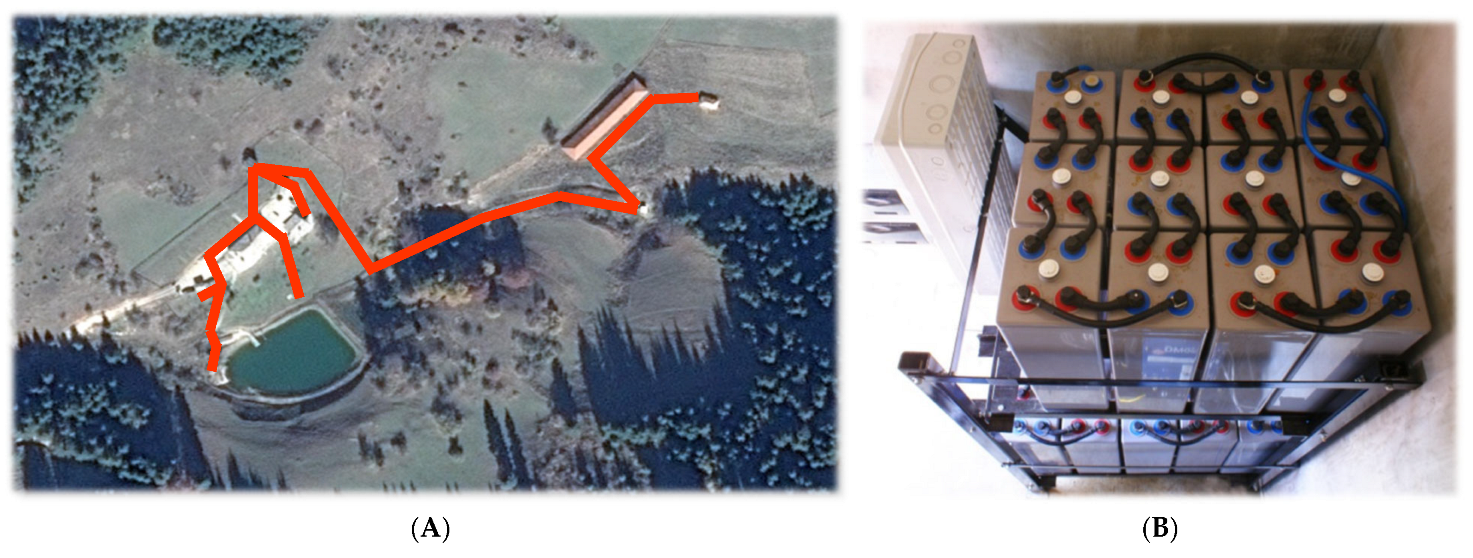
To demonstrate and validate the methodologies noted, a real-life data from the BESS of a grid-forming inverter of an autonomous microgrid is used. The microgrid is one of the test sites of the real-life living laboratory of the Power System Stability Laboratory (PSSL) of TU-Sofia. The autonomous microgrid (Figure 1A) consists of 54 V DC, 43 kWh battery storage (Figure 1B), an 8 kW bidirectional hybrid inverter with grid-forming and grid-supporting capability, one rooftop (2.3 kW) and one facade (2 kW) PV generator, a 3 kW hydro generator (HG) with 22 kWh unidirectional storage, a main 12 kW and auxiliary 4 kW diesel generators (DGs) and ~230 V AC grid (designated by the red lines on Figure 1A), which is feeding several houses, a small chapel, and five other buildings in the Rhodope mountains, Bulgaria [58].

The 54 V DC bus is formed by 27 pc. 2 V, 800 Ah OPzV batteries.

Under normal operational conditions, the PV generators feed the DC bus and charge the surplus power in the BESS.

The grid-forming unit converts the DC bus power and energy into AC, thus forming the ~230 V AC grid and serving the AC load.

5. Data Description and Pre-Processing

The data used are measured over 356 days from the 1st of January 2019 to the 22nd of December 2019. The recordings are averaged and stored every minute, providing 1440 measurements per day and 512,640 recordings in total. The measured parameters are the battery voltage and current, battery SOC (as estimated by the inverter), inverter voltage and current, AC input source power, AC output (load) power, battery temperature, and others.

After data acquisition and pre-processing, it was found that the total number of available recordings is 512,636, i.e., four are missing. Additionally, there are 67 invalid recordings with NaN values for all parameters. The missing and invalid NaN recordings represent 0.014% of the total 512,640 recordings, which is considered small. These recordings are removed from the data. The study is performed using the remaining 512,569 recordings, and the data are normalized using MinMaxScaler.

The fast and complex interactions between the system components, such as BESS, autonomous inverter, loads, PV generators, hydro generator, auxiliary diesel generator, etc., determine the rapid and significant changes of the parameters measured and stored for each 1 min time step. Due to this, when checking the data using the Z-score (standard score) method, the results show 52,065 recordings with outliers, which represents a significant share (10.16%) of the total recordings. After careful and extensive research of each parameter separately and also combined with the other parameters, it has been found that this significant share is a direct result of the physical nature of the processes. Thus, all the data are processed.

As a next step, a table of the linear correlations for the full dataset is calculated and analyzed. The linear correlation between the battery voltage U_dc and the other parameters shows relatively high positive correlation coefficient values of more than 0.74 for the battery current I_dc, 0.651 for the AC input source power, 0.516 for the temperature, and 0.112 for the AC output (load) power P_load. This could lead to the conclusion that the regression models included in this study might offer good results.

6. Training Process

6.1. Training Process Description

During the preliminary phase of the training process, a list of 37 days to be forecasted are randomly chosen. Each day from the list is used as a test period (holdout dataset). In order to prepare a model that will be tested by forecasting each day of the holdout dataset, the model is trained on all previous days before the test day (this was performed for each day separately).

In the study presented in [30], a multivariate polynomial regression model, compared with the rest of the models in the study, provided the best accuracy on forecasting regression tasks. Due to this result, the machine learning model is chosen to be based on multivariate polynomial regression. Each day from the list is used as a test period, and the training period represents all previous days before the test day. The metrics used are R² and normalized root mean square error nRMSE (normalized on the maximum achieved battery voltage).

The results of this training process for the random days set are the mean coefficient of regression R² = 0.126, and nRMSE = 1.93%, which is less than expected.

It is very possible that a data drift, similar to the one witnessed in [21], is limiting the results of this methodology. This means that using all the available data before the forecasted day for training could reduce the accuracy. Considering the relatively high correlation between the dependent and independent parameters, it was considered that it would be useful to navigate the research process in another direction.

This led to the concept of adding an optimization search to determine the optimal (or close to optimal) training period length (and using it afterwards). The chosen training length periods to compare are 15, 30, 60, and 90 days before the predicted day.

During the second stage of the training process, the data are divided into a train, validation, and test sets. The validation and test sets consist of a single day each, or 1440 recordings, and the training set length is 15, 30, 60, or 90 days.

The primary goal of this study is to compare the performance of MR, FNN, and decision-tree-based gradient boosting models (XGBoost, CatBoost, LightGBM), optimized for battery voltage forecasting in photovoltaic systems. A methodology for building an FNN model with a test R² as high as possible and an nRMSE as low as possible is proposed. The optimization of the hyperparameters of the gradient boosting methods is implemented. Additionally, a methodology for finding the optimal hyperparameter of MR with and without polynomial features is proposed and realized. In addition, an investigation how different training periods influence model performance, without assuming in advance whether the optimal training duration is model-dependent is conducted.

The research is divided into three branches—machine learning multiple linear regression analysis, deep learning FNN analysis, and gradient boosting regression analysis. Machine learning multiple linear regression analysis consists of the implementation of ML MR and ML MR with polynomial features. The latter includes grid search for optimal-degree poly-features. Deep learning FNN analysis consists of the implementation of the FNN model and a stacked ensemble of FNNs with an FNN as the main model. The hyperparameters of the single FNN and the ensemble of FNNs are optimized. The gradient boosting regression analysis consists of single models and stacked heterogeneous ensemble models with hyperparameters optimization and implementation.

6.1.1. Machine Learning Multiple Linear Regression Training

As a part of the machine learning multiple linear regression training process, a multiple linear regression model and multiple linear regression with polynomial features model are compared.

First, MR is run for a single day (train, validation, and test sets are extracted for a single day)—Figure 1. Then, as a pre-check, MR is run on the whole dataset (80/10/10—train/validation/test set).

In order to obtain the predictions of the MR, its model is run for 37 days, with four different training lengths for each day.

The implementation of MR with polynomial features requires a hyperparameter optimization search. The optimized parameters are the degree of the poly-features and the interaction between parameters.

The search for the optimal polynomial feature degree is realized with a k-fold cross-validation (k = 5) grid search. The range of possible degrees is 1 to 6; the interaction parameter is “with” and “without” interaction. The highest average result of the cross-validation provides the optimal hyperparameters, which are used for the prediction in the MR with PF model.

The prediction results of the multiple linear regression model with the optimal polynomial features and the results of the simple multiple linear regression models are calculated for a list of n number of days, n = 37, based on model training with different training periods for the forecasted day—15-, 30-, 60-, and 90-day training sets. This is implemented for each day of the list of the holdout dataset. For example, if day 100 of the recorded data is forecasted, then day 100 is used for the test data, and day 99 is used for the validation data. Each model calculates and trains four times for the given day, with four different training periods (datasets). For example, when training with 15 days, the training period is the 15 days before the validation period.

6.1.2. Deep Learning Feedforward Neural Network Training

The next stage in the research is deep learning training process. It is divided into two main parts—creating and optimizing a single-FNN model, and creating and optimizing a stacked ensemble model.

The ensemble consists of two layers—one with n base FNN models stacked together, and a second layer that consists of a main model, also an FNN.

Due to this, one of the main aims of the deep learning analysis is to implement a methodology to find an FNN, optimal or close to optimal, for the recorded data.

In order to find the optimal (or as close as possible to the optimal) hyperparameters of the feedforward neural network, a Bayesian hyperparameter optimization is run [59]. Four hyperparameters—learning rate, number of neuron nodes, number of layers, and activation function—are studied within pre-set limits.

The Bayesian grid search limits for the hyperparameter optimization of the base ensemble model are learning rate between 0.000001 and 0.1, number of neuron layers between 4 and 14, number of neurons per layer between 24 and 1024, and activation function between “ReLU” and “sigmoid”.

It was noted empirically during the search that after around 30 epochs, the neural network tends to overfit the training set, which reduces the accuracy of the results on the validation set (main monitored metrics are R squared and nRMSE). Due to this, the number of epochs for the hyperparameter optimization search and the actual predictions is set to 30.

After the hyperparameters of the single FNN are chosen, the predictions of the FNN model are implemented for every day of the chosen 37 days. For every day, a cycle is creating one by one, totaling 20 FNN models, with the chosen hyperparameters and 30 max epochs.

The goal of the cycle is to find the best of the created models and use it for the prediction for the given day. The cycle will save every model that is better than the previous best. The cycle, after finding the best of the 20 created models, will load it, use it for predictions, and store it.

In order to stop every model at its best epoch (after some waiting epochs), and eventually, the best trained model at its best epoch, an early stopping callback is used. Usually, with the default early stopping callback functions, the best epoch is found by monitoring either the lowest error on the training set or the lowest error on the validation set.

It was noted during the research that if the stopping callback monitors only the metrics of the validation set, then the model tends to achieve very high accuracy of the results on the validation set (which is a single day)—0.96, 0.98, and very low on the training set—any number from around 0.20 to 0.70. On the other hand, if the callback function monitors only the training set error, then the model overfits the training data, achieving very good results on the training set and lower results on the validation set.

Achieving good metrics on the validation set is a good predictor for achieving good results on the test set, (the data unseen by the model), if combined with good results on the training set. However, if the results on training set are not good enough, then this means that the model did not “understand” the dependences and connections between the independent variables and the dependent one. This increases the possibility of bad prediction results on the test set and is a good predictor for the low generalization of the model.

For this reason, it was considered that monitoring both training and validation metrics will be beneficial for this study. Since the default and known early stopping functions provide only training or only validation monitoring separately, a customized early stopping callback function is created to fulfill the abovementioned combined functionality.

This custom-made stopping callback could monitor one or more metrics, for both the training and validation sets, with pre-set minimum values (for example 0.75 R²). The trained model will be saved, only if it achieves better accuracy than the previous best R² results on both the training and validation sets.

The custom early stopping considers a model better than the previous one, only when the results of all metrics for the training set and validation are better than the previous values—for example, the R² on the training and validation sets of the currently trained model are better than the R² on the training and validation sets of the previous best model.

This sets some limits on the research due to omitting the models that achieve, for example, a 5% better validation R² and only a 0.1% lower training R² (if there are such models). It is considered in this research that adding a margin parameter to the custom early stopping function could be an area for future investigation.

Additionally, the custom early stopping function provides some pruning capabilities. It was noted during the training process that if the R² on the first epoch is lower than a certain value, then the trained FNN will not converge. Due to this, a pruning capability was included. If the R² for the first epoch is calculated below a certain value, then the training of the current FNN is stopped, and the training process continues with the next FNN. This leads to considerable computation process improvement.

The next part of the deep learning analysis is to study the additional possibility for results optimization to a homogeneous ensemble algorithm of a feedforward neural network model and to check its predictions on the 37 randomly chosen days. The homogeneous ensemble models are expected to improve the prediction abilities of a single model, as they consist of multiple base learner models and combine their results. The ensemble model is included in this study for comparison purposes only.

The same FNN model, with hyperparameters optimized with Bayesian search, is used as the base model. A number of k models are created, and their results are compared with the pre-set metric minimal values. Only the ones that achieved an R² and nRMSE on the training and validation sets that are higher than these pre-set minimum values—for example, 0.75 for R²—are saved and included in the stacked ensemble. When the homogeneous ensemble model is run for training, the saved base models are loaded and stacked together to form the first level of the ensemble. The first level of the ensemble (pre-trained base models) receives the training data and calculates predictions. Each base model provides its own prediction. These predictions are provided as input values to the second level of the ensemble model, which is the main model.

Based on the input predictions, the main model calculates its final forecast.

In order to create the main model, an FNN of its hyperparameters has been optimized using a second Bayesian search. As before, the researched parameters are learning rate, number of neuron nodes, number of layers, activation function, within preset limits.

The Bayesian search limits for the hyperparameter optimization of the main ensemble model are learning rate between 0.000001 and 0.1, number of neuron layers between 4 and 14, number of neurons per layer between 24 to 1024, and activation function between “ReLU” and “sigmoid”. The proposed base FNN consists of 12 dense layers, with a total 240,257 parameters. The metrics used are mean absolute error, mean square error, and coefficient of regression [60].

As mentioned above, several training period lengths are used in the study. It allows for research on the optimal training period for the models included. The research is carried out in parallel with the training and comparison of the models studied.

As proposed in [21], too long training periods could increase the error, mainly due to meteorological data drift—the PV generation model trained on winter days and temperatures will provide high error and low R² when tested on summer days. The proposed study on the optimal training length tries to avoid similar effects or different battery reactions due to the different season temperature. Also, it deserves to be noted that long training periods require more computation time and resources.

The gradient method used in the FNN training is Adam, with its exponential moving average variant: AMSGrad [61]. Cycling learning rate optimization [62,63] is also included in the optimization process.

6.1.3. Gradient Boosting Regression Training

Another part of the study is gradient boosting regression training process. In this part, a hyperparameter optimization for the chosen algorithms—XGBoost, CatBoost, and LightGMB—is implemented via Bayesian optimization.

Regarding XGBoost, the optimized hyperparameters with their limits are max depth (between 1 and 10), learning rate (between 0.0001 and 1), n_estimators (between 50 and 1000), min_child_weight (between 1 and 10), gamma (between 0.01 and 1), subsample (between 0.01 and 1), colsample bytree (between 0.01 and 1), reg_alpha (between 0.01 and 1), and reg_lambda (between 0.01 and 1). The number of lags is zero.

For CatBoost, the optimized hyperparameters with their limits are learning rate (between 0.0001 and 0.1), depth (between 1 and 10), subsample (between 0.01 and 1), colsample bylevel (between 0.05 and 1), and min_data_in_leaf (between 1 and 100). The number of lags is zero.

As for LightGBM, the optimized hyperparameters with their limits are learning rate (between 0.001 and 0.1), n_leaves (between 2 and 1000), subsample (between 0.01 and 1), colsample_bytree (between 0.05 and 1), and min_data_in_leaf (between 1 and 100). The number of lags is zero.

The chosen training length for the optimization process is 15 days.

The next part of the gradient boosting regression analysis is to study the additional possibility for results optimization to create a heterogeneous stacked ensemble model of the three decision tree models as base models (and several different algorithms for main models) and check its predictions on the 37 randomly chosen days. The heterogeneous ensemble models are expected to improve the prediction abilities of a single model, as they consist of multiple base learner models and combine their results.

The same DT models, with the optimized Bayesian hyperparameter search, are used as base models. When the heterogeneous ensemble model is run for training, the DTs are stacked together in order to form the first level of the ensemble.

Four algorithms are used as the main models—XGBoost, CatBoost, LightGBM, and linear regression. In order to optimize the hyperparameters of each main model, another Bayesian search is implemented, with the same parameters and limits as for single models.

The trained base models provide their predictions for the training and validation sets for each of the chosen days. The predictions of the three base DT models are combined into training and validation sets for the hyperparameter optimization of each main model.

As before, several training period lengths are used for the calculation.

6.2. Training Process Validation and Testing

6.2.1. Machine Learning Multiple Linear Regression Analysis

The results of a simple multiple linear regression with a 10% test set are R² equals 0.60625, RMSE equals 1.39 V, and nRMSE equals 2.32%. The results may be influenced by specific conditions or data shifts in the last 10% of the recordings.

This makes it reasonable to use k-fold cross-validation. The grid search for MR with PF is for 6 degrees and with/without interactions, which equals 12 combinations.

The k-fold cross (k = 5)-polynomial grid search calculations show that the MR with PR’s best results are for the third degree. The results of R² are [0.880, 0.897, 0.886, 0.891, 0.692], with an average result of R² 0.849. If the k-folds are 25, then the best average R² is 0.793, and the best degree is fourth. In the case of k = 3, the average R² is 0.868; the best degree is third. These results support the conclusion that the smaller the test period, the bigger the data drift with the rest of the data and the higher the error. In this study, the test period is a single day, which makes it reasonable to search for an optimal training period.

6.2.2. Deep Learning Feedforward Neural Network Analysis

The analysis of the FNN and the grid search is designed to allow the model to be accurately matched with the main parameters (battery current, P_load, P_gen, and battery temperature T). The rest of the parameters are harder to predict and use in practical model applications. Also, including the additional parameters makes the model overfit the training set and reduces accuracy on the test set. The results of the FNN trained on the full set of eight parameters are better than those from the smaller practical set of four parameters. However, given the fact that the additional four parameters are much harder to use in practical prediction, it could be assumed that for most applications, the results with the four main parameters are practically acceptable.

As a first step of the deep learning FNN analysis, a Bayesian search is implemented for the optimal values of some of the main hyperparameters of a single FNN model—learning rate, number of dense layers, number of dense nodes, and activation function. A hyperparameter set is considered better than the previous one if it improves the previous R² for the validation period.

The results are optimal learning rate—7.277 × 10⁻⁵, optimal number of dense layers—10, optimal neurons in layer—166, and optimal activation function—ReLU (rectifier linear unit). The FNNs in the next step of the research are based on this optimal hyperparameter search.

The next step is to compute the results of a single FNN model, trained with a customized early stopping function, for each of the 37 randomly chosen days with the four training periods.

After implementing the training, optimization, and predictions (with the four training periods) with a single-FNN model, the next step of the study is research on an ensemble of FNNs. The procedure is implemented to allow for the inclusion of a given number of base FNNs. This will enable future research on the optimal number of base learner FNNs. The base FNNs are pre-trained and saved only if they meet preset metric criteria—for example, FNNs that achieved an R² higher than 0.75. This means that if the number of base learners is specified to be n = 40 for the training/creating process, then only the models that achieve better results on the metric will be saved, stored, and used in the ensemble learning part of the study.

The Bayesian search limits for the optimized parameters of the main ensemble model are the learning rate between 0.000001 and 0.1, the number of neuron layers between 4 and 14, the number of neurons per layer between 24 and 1024, and the activation function between “ReLU” and “sigmoid”.

The best Bayesian grid search result from 50 iterations (n_calls = 50) is a learning rate of 0.0028, a number of FNN layers of 14, a number of neurons per layer of 994, and the activation function ReLU. It might be expected that the calculated hyperparameters could be closer to optimal with a higher number of iterations.

The resulting hyperparameters from the Bayesian grid search are used to create the main FNN model of the ensemble model of stacked FNNs. Then, for each day in the list of days, the stacked ensemble model is trained with different lengths of the training period—15, 30, 60, and 90 days.

The base FNN learners are trained on a given single day, and the ones that meet the preset criteria for accuracy are saved and used in the stacked ensemble.

Only the main model of the ensemble is trained on 37 random days.

In addition, polynomial features are created with the optimal (for the MR with PF model) third degree and fed as inputs for the FNN model. This is tested for several days only, and the results of MR PF are considerably higher than those of FNN with PF. This is implemented for testing purposes, and due to the low results, this research path is not continued.

6.2.3. Gradient Boosting Regression Analysis

The gradient boosting regression models use the same four parameters—battery current, P_load, P_gen and battery temperature T—as input data.

In this part of the study, the hyperparameters of the implemented models, based on XGBoost, CatBoost, and LightGBM, are optimized via Bayesian optimization.

The values of the optimized hyperparameters of XGBoost are max depth of 5, learning rate of 0.02562, n_estimators of 718, min_child_weight of 2, gamma of 0.84919, subsample of 0.060705, colsample bytree of 0.90312, reg_alpha of 0.30347, and reg_lambda of 0.92049. The number of lags is zero.

For CatBoost, the optimized hyperparameters and their values are learning rate of 0.09935, depth of 6, subsample of 0.80637, colsample bylevel of 0.60244, and min_data_in_leaf of 97. The number of lags is zero.

As for LightGBM, the optimized hyperparameter values are learning rate of 0.03655, n_leaves of 262, subsample of 0.78, colsample_bytree of 0.1184, and min_data_in_leaf of 97. The number of lags is zero.

A consequent part of the study is to implement ensembles from the three DT algorithms as base models and four main models—XGBoost, CatBoost, LightGBM, and linear regression model.

In order to create the first level of the ensemble, the three implemented DT models, with their optimized hyperparameters, are stacked together. Their predictions for the forecasted parameter—battery voltage—form the input datasets for the main models. The training set is created with predictions based on calculations with the training values of the four input parameters. The validation and test sets are based on calculations with the validation and test values, respectively.

The hyperparameters of the four chosen algorithms for the main model are optimized with the use of the created training and validation sets of predictions.

The values of the optimized hyperparameters of the XGBoost main model are max depth of 51, learning rate of 0.34848, n_estimators of 805, min_child_weight of 2, gamma of 0.32143, subsample of 0.99891, colsample bytree of 0.79738, reg_alpha of 0.41169, and reg_lambda of 0.12187. The number of lags is zero.

For the CatBoost main ensemble model, the optimized hyperparameters and their values are learning rate of 0.05498, depth of 5, subsample of 0.36544, colsample bylevel of 0.94349, and min_data_in_leaf of 80. The number of lags is zero.

As for the LightGBM main model, the optimized hyperparameters values are learning rate of 0.00418, n_leaves of 813, subsample of 0.11303, colsample_bytree of 0.63397, min_data_in_leaf of 22. The number of lags is zero.

As for the linear regression model, the optimized hyperparameters values are coefficient for XGBoost base model of 0.05130, coefficient for LightGBM base model of −0.0672, coefficient for CatBoost base model of 0.5595, and intercept of −0.2963.

7. Results and Analysis

The models and training process are realized with Tensorflow and other ML libraries.

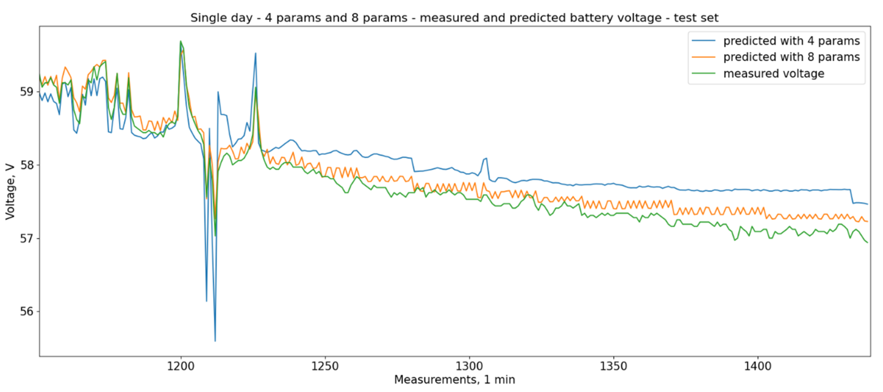
Figure 2 shows the calculated and measured values for the test period for a single day with four parameters and eight parameters for a test period of 200 time steps and a 1 min time step. The formatting is the same. It could be noticed that the prediction based on eight parameters is closer to the measured values, but the additional parameters are harder to predict and use in practical situations.

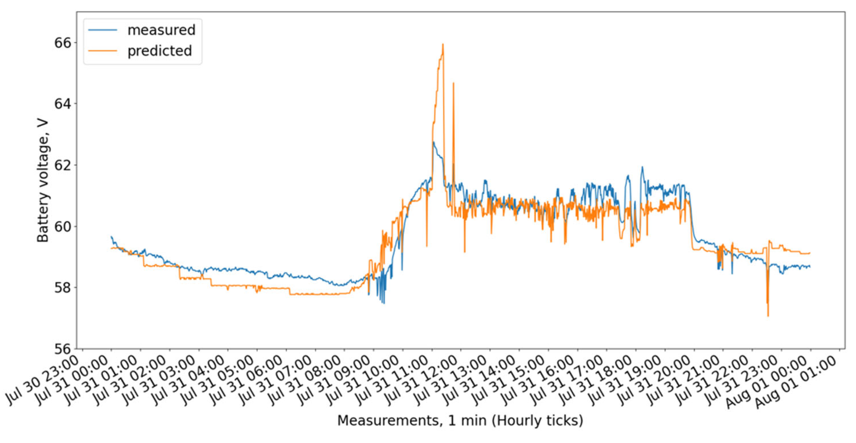
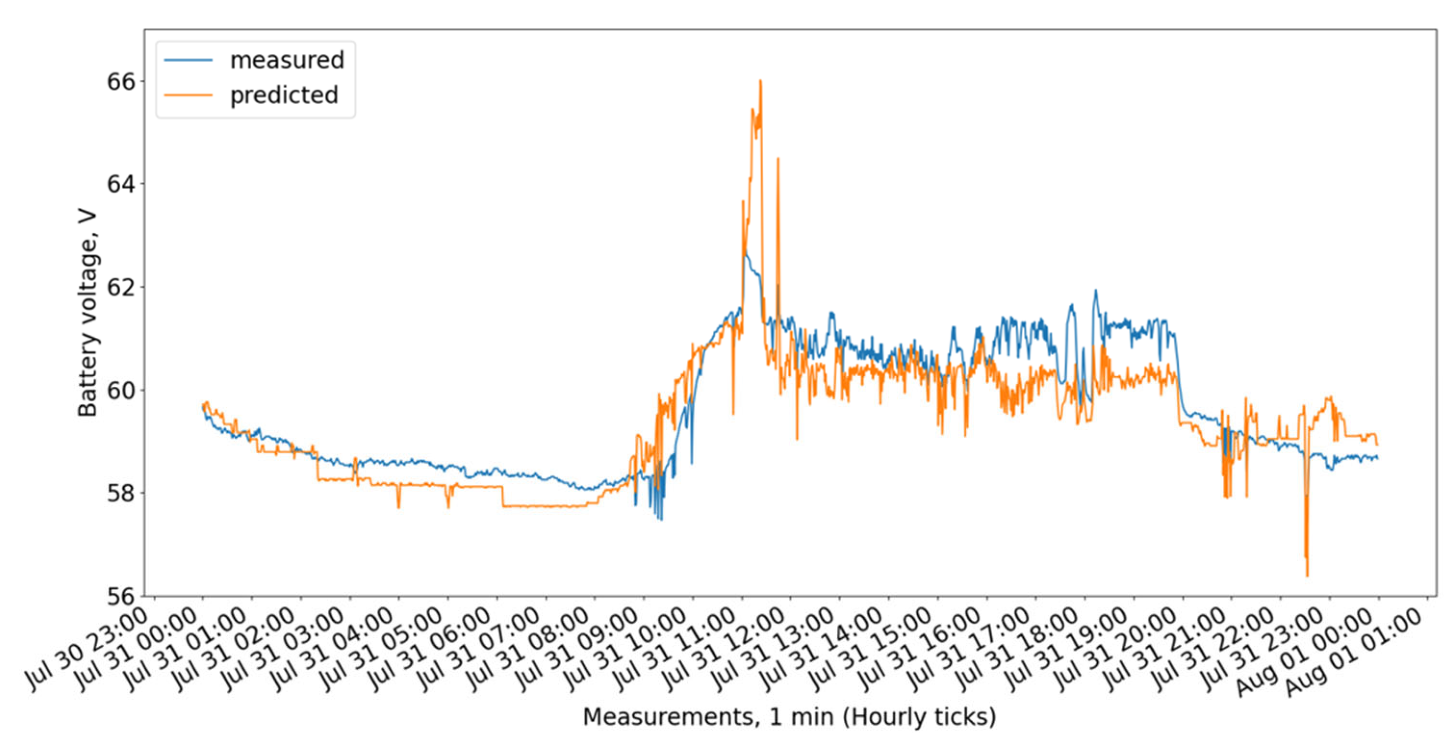
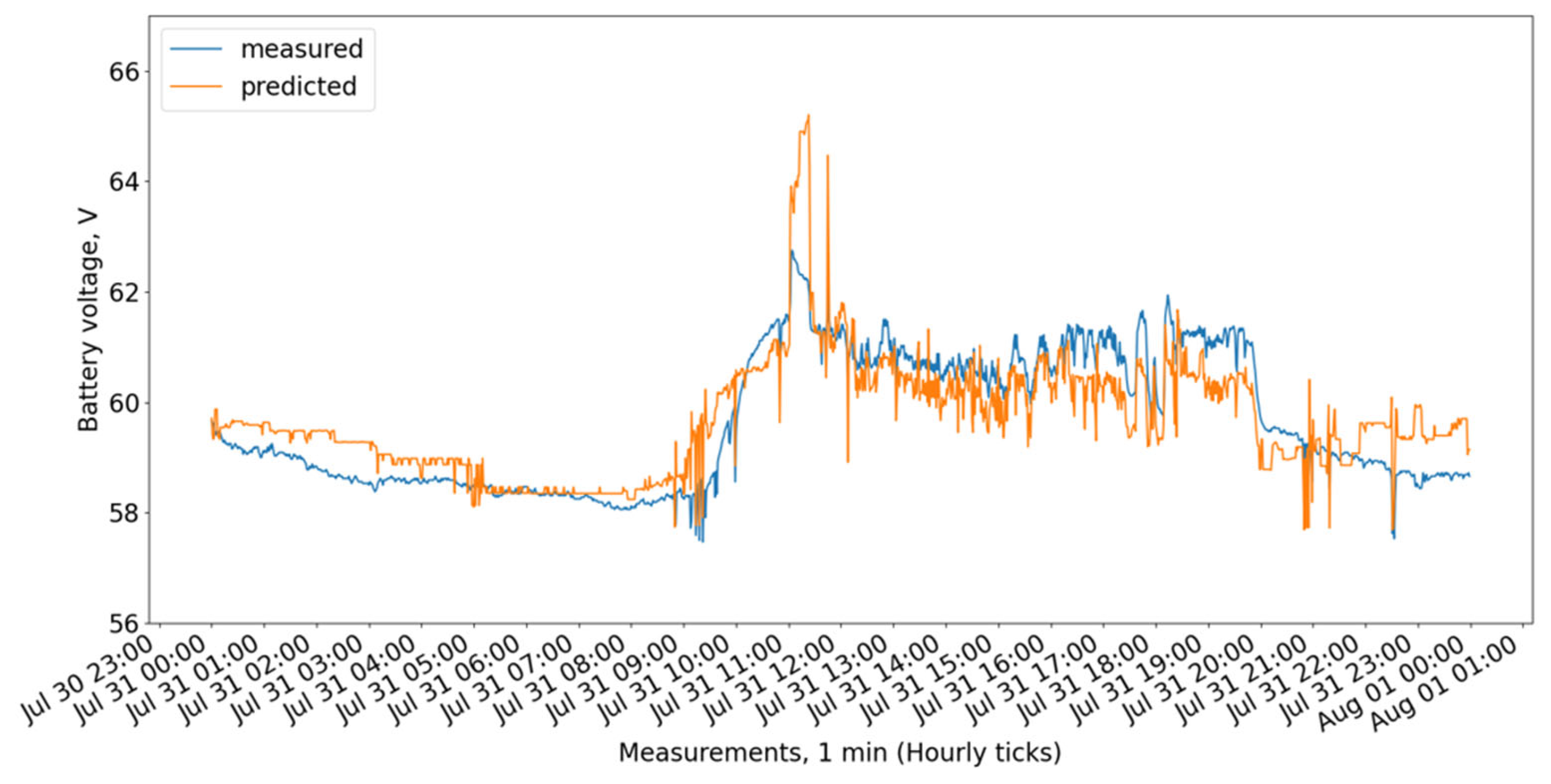
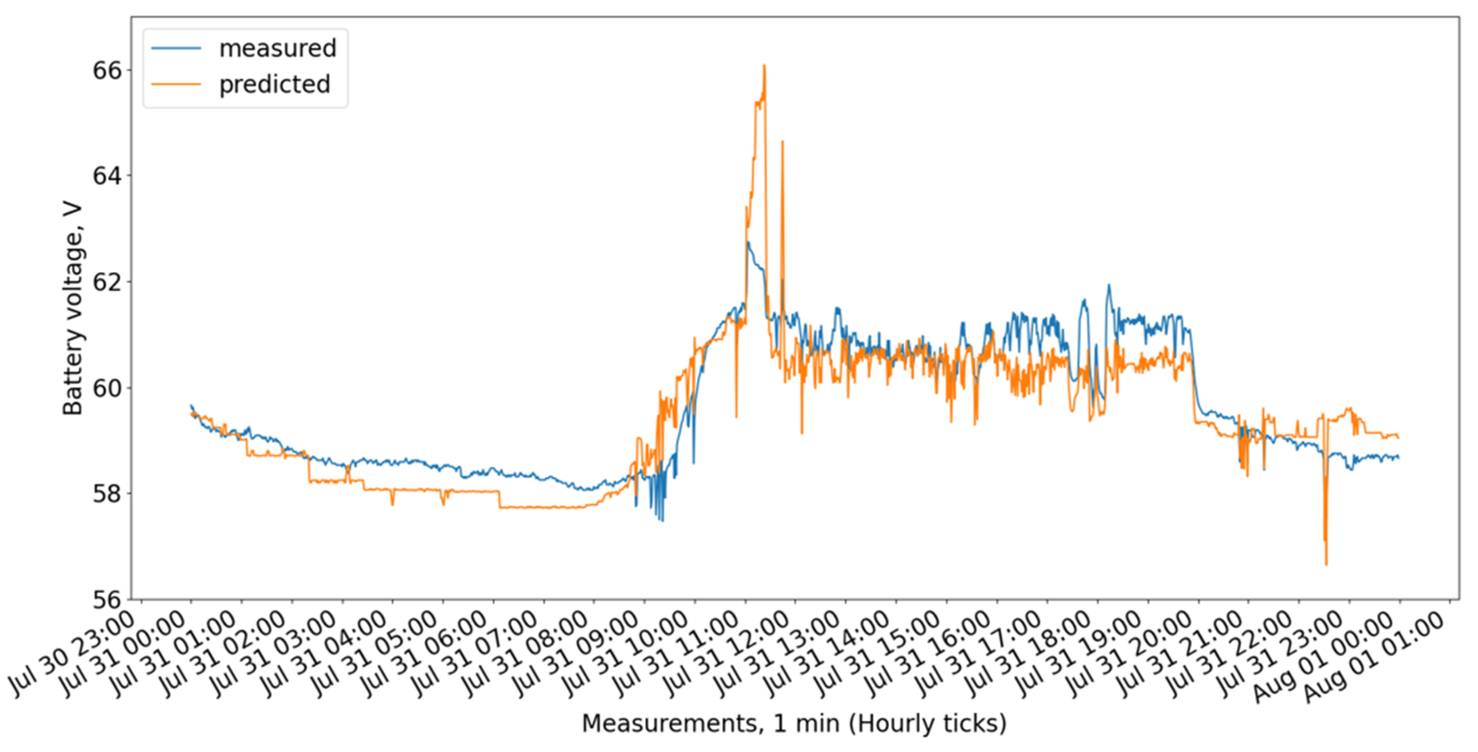
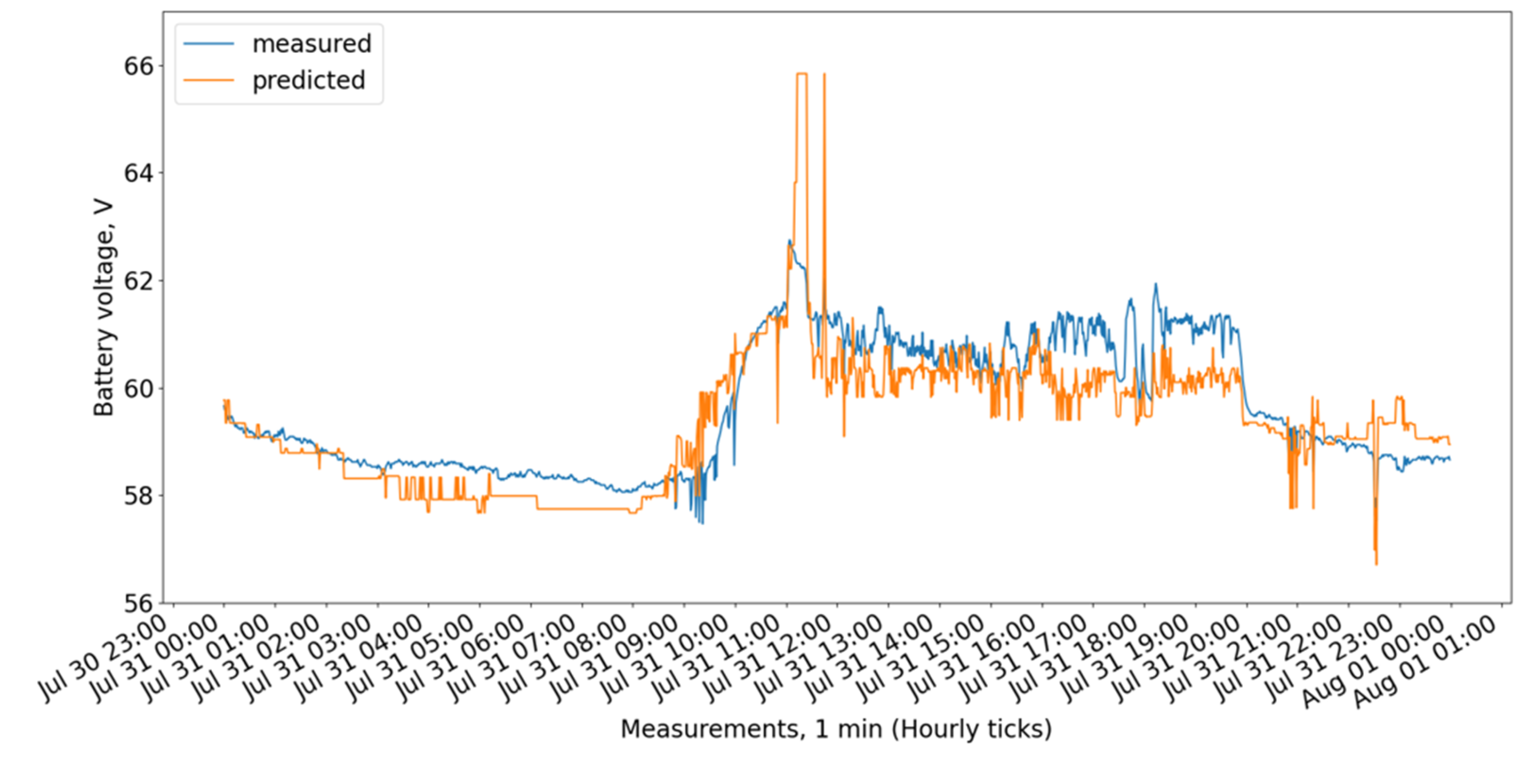
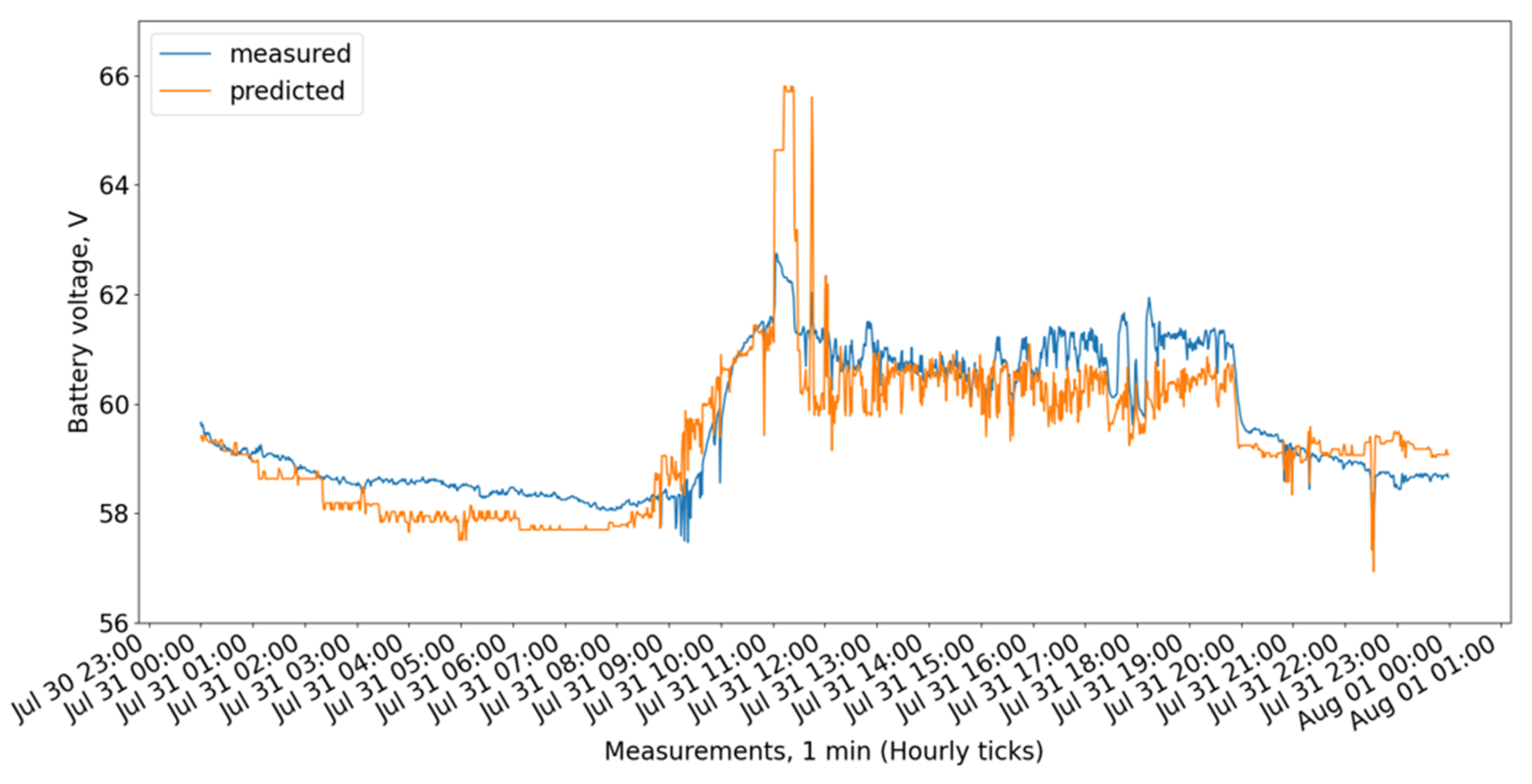
Figure 3, Figure 4, Figure 5, Figure 6, Figure 7, Figure 8 and Figure 9 show the measured and predicted battery voltage, calculated for the 15-day training period correspondingly using the CatBoost, XGBoost, LightGBM, 3 DT + LR ensemble, 3 DT + CatBoost ensemble, 3 DT + XGBoost ensemble, and 3 DT + LightGBM ensemble models.

While the CatBoost, XGBoost, and 3 DT + LR ensemble models show similar behavior offering the highest accuracy, the LightGBM exhibits a larger difference between forecasted and measured values.

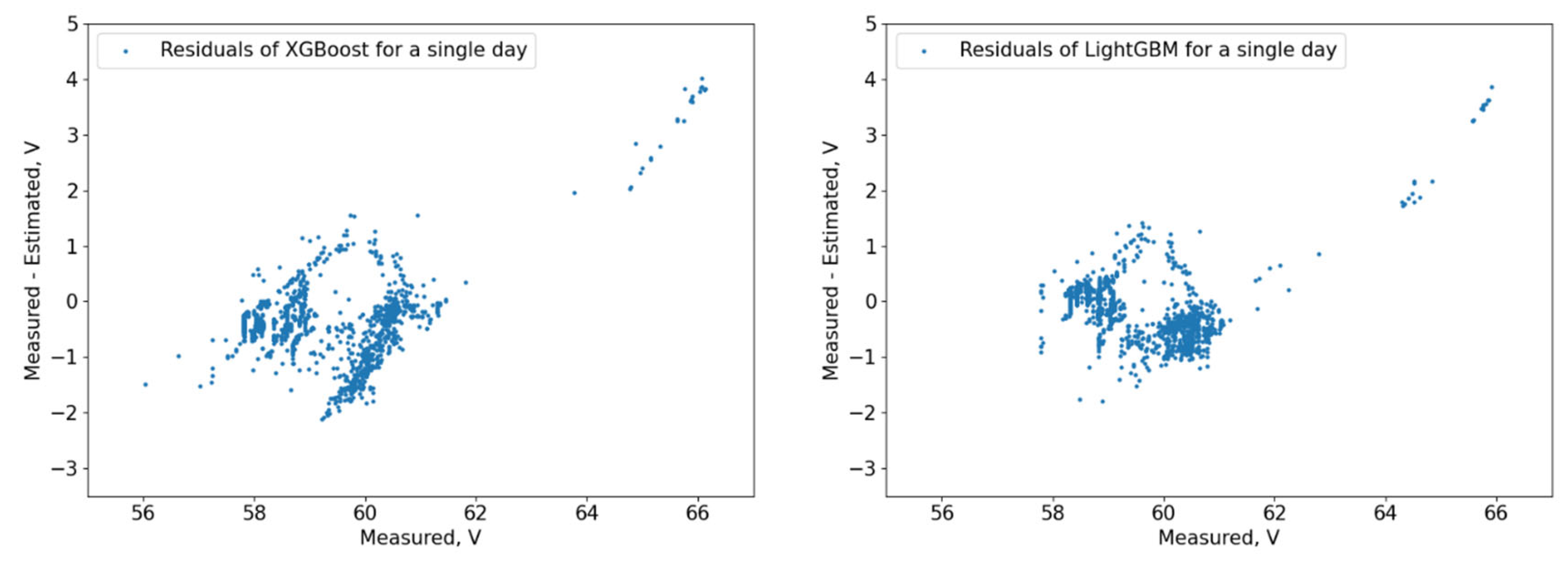
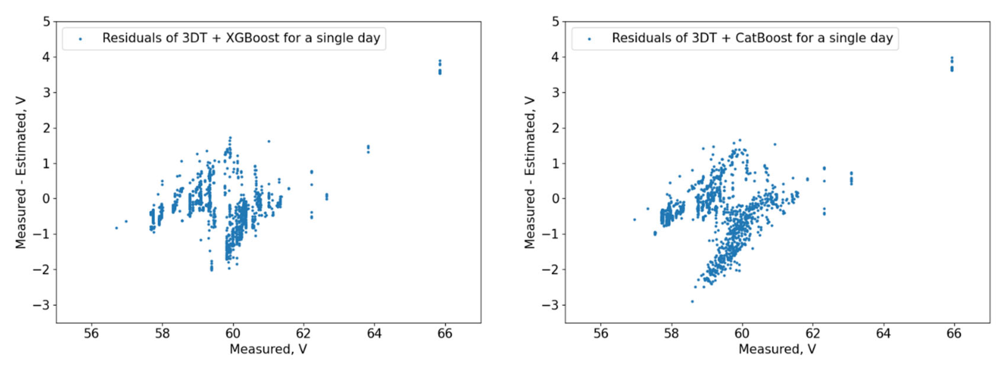
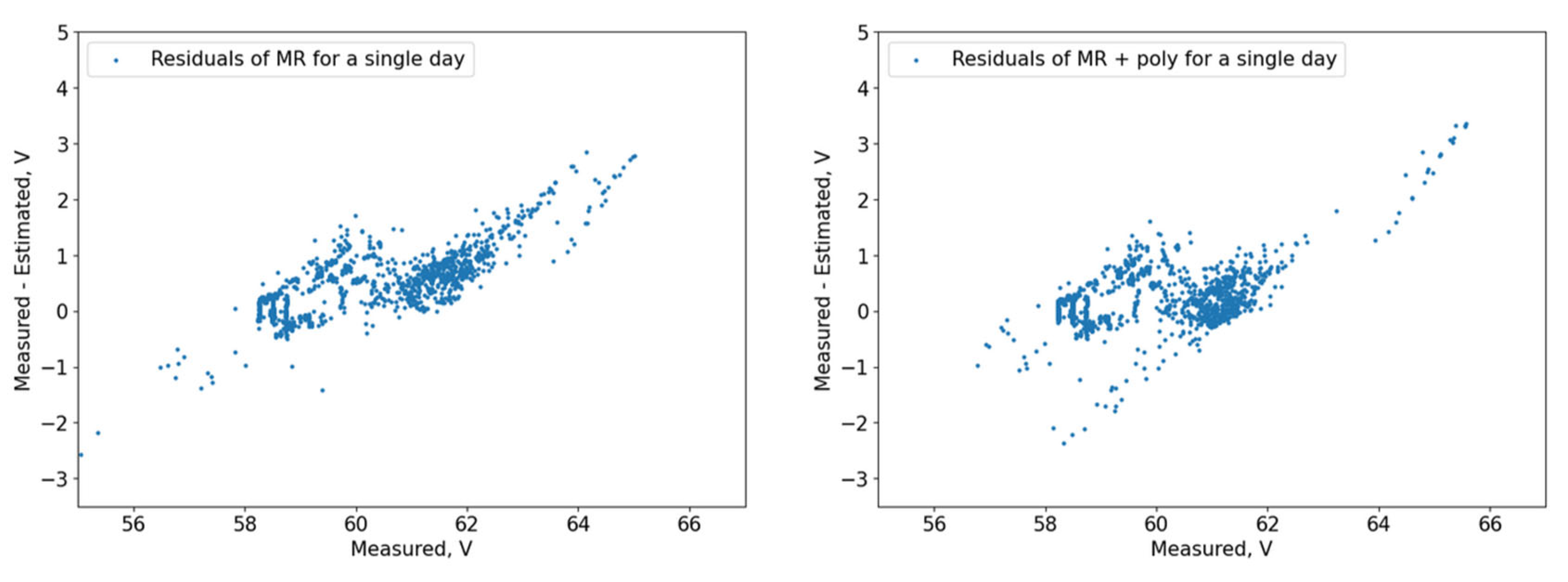
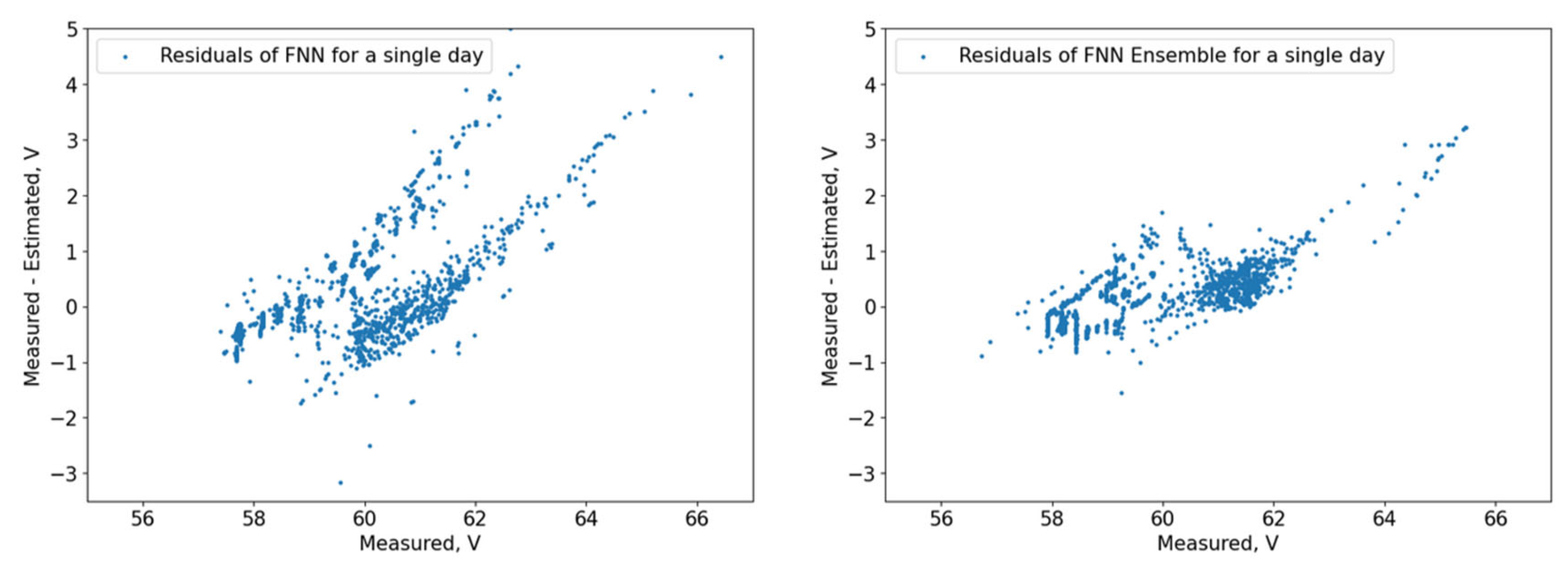
The residuals (Figure 10, Figure 11, Figure 12, Figure 13, Figure 14 and Figure 15) show that the models capture different dependencies between the input parameters and the forecasted variable. It can be noted that the residuals of the 3 DT + LR ensemble, CatBoost, and XGBoost are well grouped around the zero-point area, while others like FNN, MR, and the ensemble of FNNs are more dispersed with much more deviating results.

Table 1. Results for training, validation, and testing process.

Model Type	Training Period, Days Before	Train R2	Val R2	Test R2	nRMSE Train, %	nRMSE Val, %	nRMSE Test, %
MR	15	0.756	0.710	0.614	1.514	1.662	1.563
	30	0.734	0.645	0.598	1.618	1.818	1.670
	60	0.725	0.644	0.652	1.657	1.845	1.604
	90	0.712	0.611	0.667	1.712	1.949	1.663
MR with PF	15	0.884	0.805	0.713	1.025	1.292	1.278
	30	0.853	0.729	0.660	1.163	1.511	1.406
	60	0.809	0.705	0.717	1.340	1.585	1.344
	90	0.786	0.655	0.630	1.442	1.725	1.534
Single-FNN model	15	0.876	0.902	0.672	1.550	1.396	1.418
	30	0.843	0.902	0.706	1.436	1.317	1.384
	60	0.810	0.884	0.725	1.448	1.385	1.334
	90	0.794	0.872	0.712	1.490	1.433	1.384
FNN ensemble	15	0.793	0.831	0.683	1.409	1.360	1.425
	30	0.776	0.817	0.714	1.461	1.344	1.384
	60	0.758	0.807	0.723	1.564	1.479	1.432
	90	0.729	0.826	0.679	1.662	1.422	1.662
XGBoost model	15	0.940	0.905	0.764	0.442	0.452	0.673
	30	0.934	0.917	0.785	0.477	0.487	0.683
	60	0.912	0.872	0.732	0.555	0.605	0.723
	90	0.902	0.857	0.737	0.592	0.675	0.755
CatBoost model	15	0.941	0.907	0.773	0.437	0.443	0.689
	30	0.923	0.903	0.772	0.518	0.523	0.662
	60	0.898	0.854	0.759	0.598	0.637	0.712
	90	0.887	0.838	0.757	0.638	0.718	0.745
LightGBM model	15	0.875	0.851	0.687	0.632	0.638	0.828
	30	0.861	0.835	0.701	0.693	0.689	0.802
	60	0.835	0.803	0.667	0.759	0.783	0.844
	90	0.823	0.758	0.691	0.795	0.853	0.892
3 DT + XGBoost ensemble	15	0.944	0.929	0.766	0.421	0.428	0.699
	30	0.927	0.906	0.779	0.503	0.51	0.693
	60	0.902	0.858	0.749	0.586	0.627	0.730
	90	0.891	0.841	0.747	0.627	0.707	0.763
3 DT + CatBoost ensemble	15	0.957	0.949	0.755	0.364	0.361	0.713
	30	0.941	0.926	0.777	0.448	0.449	0.696
	60	0.917	0.880	0.728	0.538	0.569	0.732
	90	0.905	0.864	0.726	0.584	0.651	0.761
3 DT + LightGBM ensemble	15	0.950	0.937	0.763	0.395	0.402	0.702
	30	0.937	0.92	0.787	0.466	0.472	0.684
	60	0.916	0.877	0.731	0.542	0.578	0.726
	90	0.906	0.865	0.729	0.58	0.647	0.759
3 DT + LR ensemble	15	0.941	0.926	0.779	0.433	0.443	0.679
	30	0.923	0.904	0.792	0.517	0.523	0.669
	60	0.898	0.852	0.741	0.601	0.648	0.711
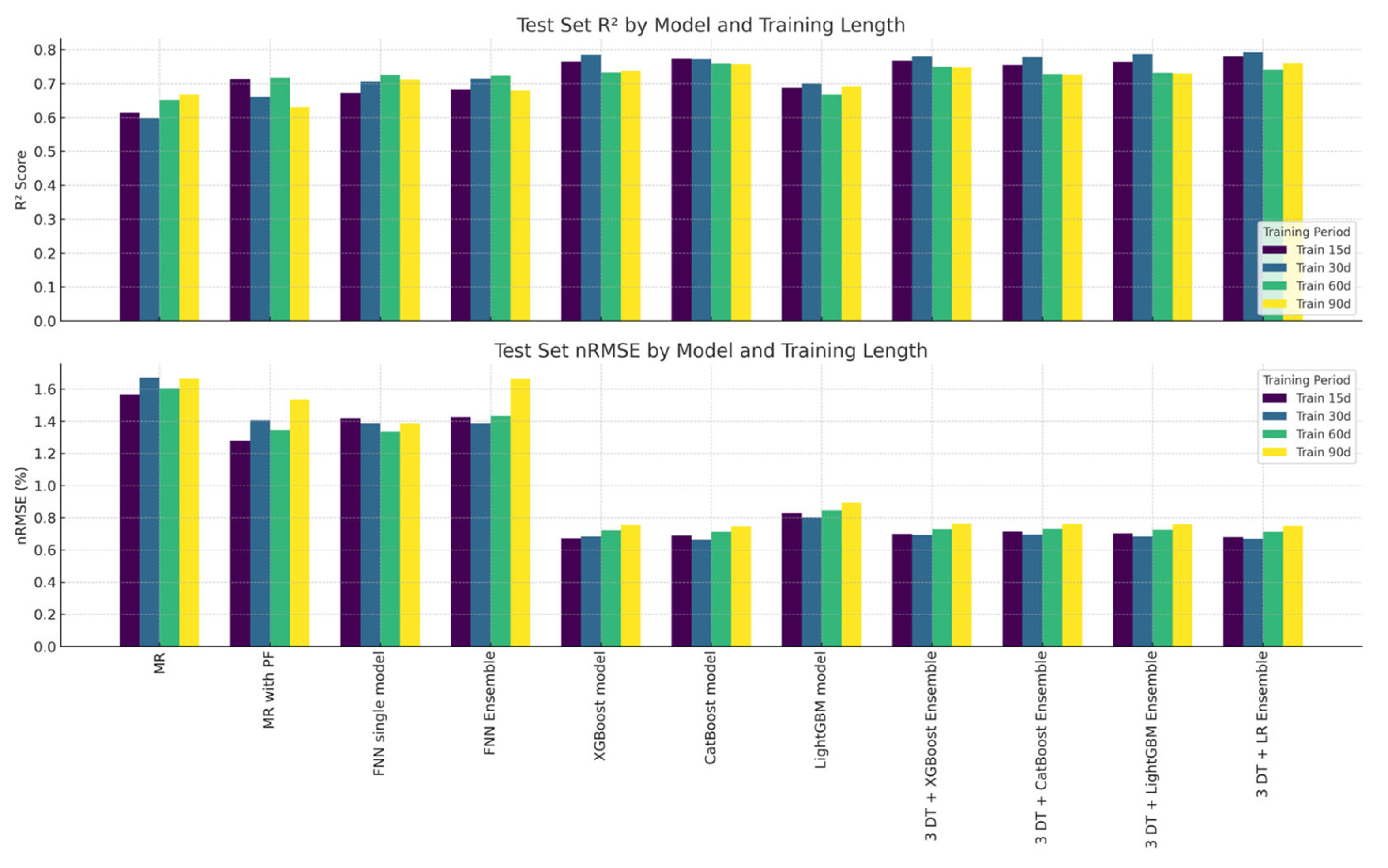
	90	0.886	0.836	0.760	0.640	0.726	0.749

shows the results of the eleven main studied models for the 37 random days of the year. It consists of the results for R² for training, validation, and test sets, and nRMSE results for training, validation, and test sets. The results are also presented for each model type’s different training period lengths. The highest achieved average result for the test set R² is for the 30-day training period for the 3 DT + LR ensemble model.

The single-FNN model, FNN ensemble, MR, and MR with polynomial features provide significantly lower results for both R² and nRMSE. Among them, the best nRMSE is from the last one, with the 15-day training period. Its R² result for 15 days is good among these four models, but the highest R² is achieved by the single-FNN model, for 60 days. The 60-day and 90-day periods, generally, provide lower results than the 15-day and 30-day period results. These data are in line with the results achieved in [30].

The average accuracy for the test R² of MR for all the training length periods (15, 30, 60, 90) is 0.632. The same accuracy for MR with polynomial features is considerably higher—0.68. For the single-FNN model, the R² is noticeably higher again—0.704. For the FNN stacked ensemble, the R² is very close to the single-FNN model—0.700.

The best result for the 37-day average nRMSE error for the test set is achieved by the CatBoost model with the 30-day training period. It can be concluded in general that the decision-tree-based models provide noticeably better results than the MR and FNN models. Assuming that the average result of a model for all training lengths could provide an indication about its performance on the data, the average result for the test nRMSE of MR for all training length periods (15, 30, 60, 90) is 1.625. The same result for MR with polynomial features is considerably better—1.39; for the single-FNN model, the results are slightly better—1.380; and for the FNN stacked ensemble, the results are worse than for the previous two models—1.475.

The results for decision-tree-based models, namely XGBoost, CatBoost, and LightGBM, for R² are 0.754, 0.765, and 0.686, respectively, and for nRMSE are 0.708, 0.702, and 0.841. This shows that the decision tree models offer better performance. CatBoost provides the best results from the DT models.

CatBoost offers slightly better results on average for all training periods than XGBoost. CatBoost appears to be a more reliable model for the available data, compared with XGBoost. On the other hand, the difference is small and could be dependent on the results for hyperparameter optimization and the chosen training periods. A higher number of iterations for hyperparameter optimization and other training periods could provide a better comparison between the two best performing models.

The heterogeneous stacked ensemble 3 DT + linear regression model provides the best test R² result, the best average R² result, and together with the CatBoost model, offers the best average result for the test nRMSE. This could be due to the fact that LR provides coefficients for the best result of the linear model, while finding the optimal hyperparameter values for the more complex DT models is more difficult. A possible future study might be to research whether the best DT model could provide better results with a higher number of Bayesian trials.

The results, presented in Table 1, are shown in a bar chart in Figure 16. The chart shows all models, in two rows. The first row shows the results of every model for test set R², for each training length—15, 30, 60, and 90 days. The second row shows the results for nRMSE of each model.

Regarding the homogeneous FNN ensemble, due to computation limits, the base FNN learners are trained only once on a single day, and not on the training days before each of the 37 days chosen. Only the main model (with loaded pre-trained base learners) is trained on the selected days. This imposes limits on the ensemble capabilities, as a big part of the model is not trained on the tested day training period. The lower results of the ensemble model when compared with the single FNN could be largely due to the above-mentioned limits.

A possible conclusion from these results is that if the base learners of a stacked ensemble model are not trained on suitable training data, then it cannot provide better results compared with the single model trained on proper data. One approach to overcome this might be to train each of the base FNN learners on different training days.

8. Discussion

This study shows that CatBoost achieves the best nRMSE, higher than the other single-DT models and the three DT ensembles. The second nRMSE result is provided by the 3 DT + LR ensemble. The third nRMSE result is provided by the XGBoost model. The best and the second best nRMSE results are based on a 30-day training period, while the third best are based on a 15-day training period.

The highest test set R² result of the study is shown by the heterogeneous 3 DT + LR ensemble, while the 3 DT + LightGBM ensemble follows closely in second. The third result is from the XGBoost model. The top three results are in the 30-day training period.

Generally, the decision-tree-based models exhibited better results compared with the FNN, ensemble of FNNs, and multiple regression models with and without polynomial features.

This could suggest that the optimal training period for this study is 30 days. This means that longer training periods are not necessary for achieving optimal prediction results.

In practical terms, when using such a model for day-ahead forecasting and considering the potential financial penalties of the energy market, nRMSE seems to be a more important metric than R². Due to this, in this research, the model with the lowest nRMSE is considered to have the highest importance for practice. In this study, the model with the lowest nRMSE test error is CatBoost (0.662%), and the ensemble of three DTs with LR closely follow (0.669%), though the latter provides much better R² metric results (0.792 compared with 0.772). Considering also that both models provide nearly the same average nRMSE result for all training periods, in practical tasks, the three DTs with LR could prove to be more useful.

This study has significant applicability for the practice by providing a prediction of real-life battery performance. This prediction allows for the optimal use of the energy stored in the BESS, smart planning of the available resources and capabilities for power system stability support, network parameter control using a converter-connected BESS, as well as smart flexible load control and peak load shifting.

The selected optimal prediction model can be further tested and compared with other hybrid and conventional models––LSTM, CNN, and other heterogeneous stacked ensembles.

This study proposes implementation for the calculation and training process, as well as a customized early stopping function for the training of NNs. As the default early stopping functions provide monitoring on a single metric—for example, nRMSE validation loss; the need to monitor both training and validation loss led to the conclusion of the development of a customized function. Additionally, it was noted empirically during the training process that many FNNs start with a very low value of R² in the first epoch and never improve. The customized function allows for the inclusion of pruning abilities—when an FNN shows a low R² in the first epoch, its training is stopped, and the training of the next one starts.

Regarding the test set size, consisting of 37 random days, which is around 10% of the available data, one possibility for future improvement is to increase the size of the test set. Due to computational resource considerations, this study was started and finished with this test set for the chosen training set lengths.

This study also proposes implementation for the calculation and optimization process for decision-tree-based models, as well as their hyperparameters for the data used. Additionally, this study proposes hyperparameter optimization and the implementation of four DT ensemble models. These models offer the best results.

9. Conclusions

This study shows a comparison between XGBoost, CatBoost and LightGBM models, three DT ensembles, the top-performing FNNs and their ensembles, MR, and MR utilizing polynomial features. Furthermore, an investigation into the ideal training duration employing the abovementioned models is proposed.

The results shown in Table 1, calculated with three DTs with an LR ensemble, lead to the conclusion that this model shows the highest performance for R² and the second best results for nRMSE amongst the included models. CatBoost offers competitive results, providing the best results for nRMSE and good results for R².

Based on the calculation results, it could be concluded that both FNNs and MR PF achieved lower accuracy in the research, with the latter showing slightly better metric results.

As part of the deep learning FNN analysis study, a Bayesian hyperparameter search is proposed, and a customized early stopping function is introduced. Also, an ensemble stacked model with a customizable size (based on the number of input base models) is proposed. The base models are generated with hyperparameters proposed by the results of the Bayesian hyperparameter search. The models that pass an accuracy check implemented with the customized early stopping callback function are included in the ensemble model.

As part of the machine learning Multiple Linear Regression analysis, an MR with polynomial features is introduced, with a grid search for the optimal features of polynomial degrees.

In the gradient boosting regression analysis part, the hyperparameters of the included three single and four ensemble models are optimized via Bayesian search.

The trained models or pipelines in this study could be used as a transfer learning addition to the study performed in [64].

A promising possible future work might include a comparison with other NN types, like LSTM, CNN, or transfer learning [65,66].