Photovoltaic Power Generation Forecasting Based on Secondary Data Decomposition and Hybrid Deep Learning Model

Abstract

Accurate forecasting of photovoltaic (PV) power generation is crucial for optimizing grid operation and ensuring a reliable power supply. However, the inherent volatility and intermittency of solar energy pose significant challenges to grid stability and energy management. This paper proposes a learning model named CECSVB-LSTM, which integrates several advanced techniques: a bidirectional long short-term memory (BILSTM) network, Complete Ensemble Empirical Mode Decomposition with Adaptive Noise (CEEMDAN), variational mode decomposition (VMD), and the Sparrow Search Algorithm (CSSSA) incorporating circle chaos mapping and the Sine Cosine Algorithm. The model first uses CEEMDAN to decompose PV power data into Intrinsic Mode Functions (IMFs), capturing complex nonlinear features. Then, the CSSSA is employed to optimize VMD parameters, particularly the number of modes and the penalty factor, ensuring optimal signal decomposition. Subsequently, BILSTM is used to model time dependencies and predict future PV power output. Empirical tests on a PV dataset from an Australian solar power plant show that the proposed CECSVB-LSTM model significantly outperforms traditional single models and combination models with different decomposition methods, improving R² by more than 7.98% and reducing the root mean square error (RMSE) and mean absolute error (MAE) by at least 60% and 55%, respectively.

1. Introduction

As global energy demand continues to rise and environmental pressures intensify, the development of new energy sources has become a global consensus. The extensive use of fossil fuels not only exacerbates environmental pollution but also accelerates climate change, compelling the international community to seek cleaner and more sustainable energy solutions. In this context, the advancement of safe renewable energy technologies, such as solar photovoltaic (PV), is particularly crucial [1]. Take the large-scale power outage in Spain and Portugal on 28 April 2025 as an example. This incident affected millions of people across the two countries and parts of France. The power outage, which was mainly attributed to factors like sudden drops in solar power output and grid oscillations, led to chaos in various aspects of society, including transportation, retail, and healthcare. It vividly exposed the vulnerability of power systems when integrating high-proportion renewable energy, highlighting the importance of ensuring grid reliability during the energy transition process. According to the latest report from the International Renewable Energy Agency (IRENA), in 2023, the global installed capacity of solar PV reached 1419 gigawatts (GW), accounting for 37% of the world’s total installed renewable energy capacity. This remarkable growth not only signifies technological advancement and cost-effectiveness but also reflects the urgent global demand for clean, sustainable energy solutions.

The output power of photovoltaic (PV) generation is influenced by meteorological factors such as solar radiation, temperature, humidity, and wind speed. These fluctuations increase the uncertainty of power generation, affecting system efficiency and stability [2,3]. For example, studies have shown that optimizing the spectral allocation of solar radiation can improve the solar-to-electricity efficiency of PV cells, with efficiency reaching 20.3% when the cutoff wavelength increases to 850 nm [4]. This highlights the significant impact of solar radiation levels on PV power output, making it a critical factor in system performance. With the large-scale grid integration of PV power plants, the penetration of PV power in the grid increases, enhancing the renewable energy supply but also introducing more uncertainty. This may lead to an imbalance between power supply and demand, threatening the stability of the smart grid. Therefore, developing accurate PV power prediction models is crucial. This helps grid operators optimize scheduling strategies, improve the efficiency of renewable energy utilization, and ensure the stable operation of the power system.

Photovoltaic (PV) power forecasts can be categorized into four types based on the time horizon: ultra-short-term, short-term, medium-term, and long-term forecasts [5]. Ultra-short-term forecasts, which address power variations from a few minutes to a few hours, are critical for real-time grid scheduling and management. They typically have a resolution of 5 min [6,7] and can effectively respond to immediate power demand changes [8]. Short-term forecasts cover periods from hours to a week and are mainly used for daily power operations and dispatch planning. Medium-term forecasts span from days to months and are typically used for seasonal power demand forecasting and maintenance planning. Long-term forecasts range from a few months to several years and support energy policy-making and strategic planning for electricity markets. This hierarchical forecasting approach helps the power system manage the uncertainty and volatility of PV power generation across different time scales. This research focuses on developing an ultra-short-term PV power forecasting model to provide utilities with the ability to accurately schedule power production and enhance power reserve management. This model will enable a more effective response to immediate changes in grid demand, ensuring continuity of power supply and system stability. Current PV power prediction methods include physical methods, statistical analysis methods, and machine learning methods. Each method has its own advantages and limitations, and selecting the appropriate technique is crucial for optimizing the overall benefits of PV power generation.

Physical methods for PV power prediction establish a physical link between power output and numerical weather prediction (NWP) by incorporating the geographical location of the PV plant and the equipment characteristics (e.g., PV panels and inverters) [9]. Mayer and Gróf (2021) systematically compared 32,400 physical model chains for 16 PV plants and reported that the optimal models achieved mean absolute errors (MAEs) of 28.3–32.6% and root mean square errors (RMSEs) of 46.1–52.1% for intraday forecasts, with a 12–13% accuracy gap between the best and worst model configurations [10]. However, the accuracy of this method heavily depends on the precision of numerical weather predictions, and uncertainties and errors in weather forecasts can directly affect the reliability of the prediction results [11,12]. Statistical analysis methods perform power prediction by analyzing historical time series data, with commonly used models including the autoregressive moving average (ARMA) model, the quantile regression model, and the autoregressive integrated moving average (ARIMA) model. These methods offer advantages such as simple model construction, fast computation speed, and suitability for handling time series data with stable changes. However, PV data are highly volatile and influenced by multiple environmental factors, which may lead to significant prediction errors [13]. In recent years, machine learning methods have gained widespread attention in PV power prediction due to their strong adaptability and data processing capabilities. Pan et al. [14] proposed a support vector machine (SVM) model optimized by improved ant colony optimization (I-ACO), achieving an R² of 0.997 for ultra-short-term PV power forecasting. The model significantly improved peak load prediction accuracy (MAE reduced by 44.2% vs. raw data) and nighttime forecasting (RMSE = 0.1868). However, SVM relies on quadratic programming, leading to long training times for large datasets (e.g., 5 min resolution data over 1.5 years). Zhuo et al. [15] proposed an extreme learning machine (ELM) model, achieving high prediction accuracy through meteorological feature screening and parameter optimization, but the random initialization of its hidden layer parameters may lead to performance fluctuations and overfitting [16]. Heng [17] proposed an optimized backpropagation algorithm (BP), which has better prediction performance than comparative algorithms but is prone to falling into local optima. The long short-term memory (LSTM) network is widely used due to its advantages in time series processing, multi-input integration, and long-term memory. The authors [18] combined LSTM with a particle swarm optimization algorithm to significantly improve the accuracy of solar power generation prediction, especially across different seasons. To enhance feature extraction, the structure of deep learning models, such as LSTM and GRU, can be optimized. A study by Mellit et al. [19] showed that bidirectional LSTM (BiLSTM) and bidirectional GRU (BiGRU) perform well in short-term solar power prediction with high accuracy. These machine learning methods provide an important reference for the selection of prediction models. To improve the accuracy and reduce the training time of PV power prediction models, the literature [13] suggests using Pearson’s correlation coefficient to identify meteorological variables that are highly correlated with PV power output. This approach reduces the dimensionality of input features, thereby decreasing data complexity and training time. Additionally, data completeness and accuracy are crucial to prediction results, as missing data and noise can have negative impacts. Decomposition techniques can effectively mitigate data noise and volatility, enhancing prediction accuracy [20]. Wavelet transform (WT), a commonly used decomposition technique, relies on the selection of basis functions and thresholds, and choosing the appropriate decomposition scales is also challenging [21]. To address this, Empirical Mode Decomposition (EMD) has been proposed, which automatically decomposes signals based on time-scale features, making it suitable for nonlinear analysis and exhibiting strong adaptability [22]. However, EMD suffers from mode-mixing problems. Complete Ensemble Empirical Mode Decomposition (CEEMDAN) [23] reduces the interference of high-frequency sequences in the original series on prediction accuracy by separating these sequences, but certain high-frequency components may still affect prediction results. To further minimize the interference of high-frequency sequences, Wen et al. [24] employed a second harmonic decomposition method, using the variational mode decomposition (VMD) algorithm to further decompose high-frequency components. In recent years, researchers have explored the fusion of different models to construct hybrid prediction models to improve prediction accuracy. One study [25] proposes an integrated learning model combining LSTM, VMD, and the Multi-Strategy Optimization Dung Beetle Algorithm (MODBO) for short-term electricity load forecasting, significantly improving forecasting accuracy and efficiency and optimizing global search capability. The authors of [26] present a hybrid neural network model that significantly enhances the accuracy and stability of photovoltaic (PV) power forecasting by combining Conv-LSTM and TCN structures, effectively supporting energy management and grid stability. In [27], a TCN-ATT-LSTM transfer learning method is introduced that combines sensitive meteorological feature selection specifically for wind and solar power generation prediction, capable of quickly constructing an adaptive model and significantly improving prediction accuracy at data-scarce target sites. Although hybrid models perform well in PV power generation prediction, different parameter settings can affect the final performance of the prediction model. For instance, the choices of VMD decomposition level K and penalty coefficient α are crucial for enhancing the model’s ability to handle nonlinear and nonsmooth signals [28]. Therefore, accurately finding the right parameters is a critical step in improving prediction accuracy. In [29], the accuracy of PV power prediction is significantly enhanced by combining an improved particle swarm optimization (PSO) algorithm with a kernel-based extreme learning machine (KELM) to effectively find the optimal parameters. Additionally, optimizing neural network parameters using meta-heuristic algorithms can enhance the model’s predictive performance. Such algorithms include particle swarm optimization (PSO), gray wolf optimization (GWO), and the whale optimization algorithm (WOA), among others. In [30], researchers employed the Sparrow Search Algorithm (SSA) to improve the performance of extreme learning machine (ELM) predictions, particularly in mitigating the uncertainty caused by input weights and biases. The results indicate that the SSA exhibits better optimization performance than the traditional particle swarm optimization (PSO) algorithm, although it sometimes falls into local optima during the search process. Further research [31] optimized the search step size of the SSA by introducing the Levy flight strategy, which improved search efficiency and increased prediction accuracy.

Although research has significantly improved the accuracy of PV power generation prediction by applying various deep learning hybrid models and optimization algorithms, challenges remain in handling complex data structures, especially high-frequency data components. These high-frequency components often adversely affect the prediction performance of models. To address this, this study proposes an innovative hybrid model, CECSVB-LSTM, which integrates CEEMDAN and the Sparrow Search Algorithm (CSSSA) that incorporates Circle chaotic mapping and Sine Cosine algorithms, VMD, and BiLSTM. By combining different decomposition techniques with a bidirectional long short-term memory network, the model optimizes global search capabilities and enhances the handling of complex data structures. The main contributions and innovations are summarized as follows:

(1) The model proposed in this study takes into account the correlation characteristics with the historical patterns of the target variable and significantly enhances predictive accuracy by integrating multiple correlated variables.

(2) This study enhances the SSA through multiple strategies. Circle chaotic mapping, the Sine Cosine Algorithm (SCA), the Learning Factor Strategy, Cauchy Variation, and Variable Spiral Search Strategies are integrated to rectify VMD parameters, forming the CSSSA-VMD method. This enhancement not only optimizes VMD parameter selection but also significantly improves the algorithm’s global search capability and parameter optimization efficiency.

(3) This study innovatively proposes an initial decomposition of the signal using CEEMDAN to extract intrinsic modal functions (IMFs), effectively addressing the nonlinearity and non-stationarity of the signal. Subsequently, high-frequency signal components are further finely decomposed using CSSSA-optimized VMD to ensure the extraction of richer features. This dual decomposition strategy not only enhances the extraction of signal features but also provides richer input information for the BiLSTM prediction model. Through multi-stage signal processing and optimization, the model is better adapted to complex time series data, significantly improving prediction accuracy and reliability.

In the subsequent study, the paper is organized as follows: Section 2 details the methodologies, including CEEMDAN, VMD, the optimized Sparrow Search Algorithm (SSA), and BiLSTM. It also outlines the CECSVB-LSTM model architecture, illustrating how dual decomposition (CEEMDAN + CSSSA-optimized VMD) collaborates with BiLSTM for forecasting. Section 3 compares the proposed CECSVB-LSTM model with commonly used models and verifies its performance advantages through multiple experiments. Finally, Section 4 summarizes the research findings, draws conclusions, and looks forward to future research directions.

2. Materials and Methods

2.1. CEEMDAN

The Complete Ensemble Empirical Mode Decomposition with Adaptive Noise (CEEMDAN) is an enhancement of the EMD, EEMD, and CEEMD algorithms, designed to address the issue of mode aliasing. The photovoltaic power curve exhibits non-stationary and nonlinear characteristics. While EMD decomposition is susceptible to mode aliasing, EEMD and CEEMD mitigate this to some extent by adding random white noise. However, they still suffer from issues such as residual noise and an inconsistent number of modes. CEEMDAN improves upon these by introducing adaptive noise, which enhances the precision and stability of the decomposition, thereby ensuring the quality of signal processing. The specific steps of CEEMDAN are as follows:

(1) Add n times Gaussian white noise of the same length to the original signal $x(t)$ to construct the sequence $x_i\left(t\right)$ to be decomposed n times, where $i=1,2,3,\dots ,n$. The formula is as follows:

$$x_i(t)=x(t)+{\epsilon }_0{\omega }_i(t)$$

(1)

where ${\epsilon }_0$ is the weight coefficient of the Gaussian white noise, and ${\omega }_i(t)$ is the Gaussian white noise generated at the i-th time.

(2) Decompose $x_i\left(t\right)$ by EMD to obtain the first modal component $IM{F}_1\left(t\right)$. Repeat the decomposition n times, and take the average value to obtain the first modal component $IM{F}_1$ and residual component $r_1(t)$ of CEEMDAN, using the following equations:

$$IM{F}_1={\displaystyle \frac{1}{n}}{\displaystyle \sum _{i=1}^{n}IM{F}_1(t)=\frac{1}{n}EM{D}_1(x_i(t))}$$

(2)

$$r_1(t)=x(t)-IM{F}_1$$

(3)

(3) Add white noise to the first residual component $r_1(t)$ again and, by analogy, obtain $IM{F}_2(t)$ and $r_2(t)$, using the following equations:

$$IM{F}_2={\displaystyle \frac{1}{n}}{\displaystyle \sum _{i=1}^{n}IM{F}_2(t)}$$

(4)

$$r_2(t)=r_2(t)-IM{F}_2$$

(5)

(4) Similar to the above steps, the k-th component is obtained as follows:

$$IM{F}_k={\displaystyle \frac{1}{n}}{\displaystyle \sum _{i=1}^{n}EM{D}_1(r_{k-1}(t)+{\epsilon }_{k-1}{\mathit{EMD}}_{k-1}({\omega }_i(t)))}$$

(6)

$$r_k(t)=r_{k-1}(t)-IM{F}_k$$

(7)

where $IM{F}_k$ denotes the k-th modal component obtained by CEEMDAN decomposition, and $r_k(t)$ denotes the k-th order residual signal.

(5) Until the residual component is a monotonic signal, i.e., it cannot be decomposed further, the decomposition is stopped, and the final original signal can be expressed as:

$$x\left(t\right)={\displaystyle \sum _{i=1}^{n}IM{F}_K+R\left(t\right)}$$

(8)

where K is the number of IMF obtained by CEEMDAN decomposition, and $R(t)$ is the final residual term.

2.2. VMD

Variational modal decomposition (VMD) is a signal processing method that can effectively improve the smoothness of time series with high complexity and strong nonlinearity, decomposing them into relatively smooth subsequences containing multiple different frequency scales with good adaptability and discriminative ability. In this paper, after CEEMDAN decomposition of the photovoltaic power series, the high-frequency component still exhibits significant randomness, and its VMD decomposition can effectively reduce this randomness. The core idea of VMD is to construct and solve a variational problem. The constrained variational model is as follows:

$$\left\{\begin{array}{l}\underset{\{u_k,{\omega }_k\}}{\min }\left({\displaystyle \sum _k{‖{\partial }_t\left\{\left[\delta \left(t\right)+\frac{j}{\pi t}\right]u_k\left(t\right)\right\}{e}^{-j{\omega }_{k}t}‖}_2^2}\right)\\ s.t.{\displaystyle \sum _{k=1}^K}{u}_k=x\left(t\right)\end{array}\right.$$

(9)

where $u_k$ is the k-th component of the original signal; ${\omega }_k$ is the central frequency of the k-th IMF component; $\delta \left(t\right)$ is the Dirac function; K is the decomposition level; $j$ is the imaginary unit; ${\partial }_t$ denotes differentiation; and $x\left(t\right)$ is the original signal to be decomposed. By introducing the penalty factor $\alpha$ and the Lagrange multiplier $\lambda$, the constrained problem is transformed into an unconstrained variational problem, expressed as follows:

$$\begin{array}{r}L\left(\left\{u_k\right\},{\omega }_k,\lambda \right)=\alpha {\displaystyle \sum _k{‖{\partial }_t\left\{\left[\delta \left(t\right)+\frac{\mathrm{j}}{\pi \mathrm{t}}\right]u_k\left(t\right)\right\}{e}^{-j{\omega }_{k}t}‖}_2^2+}\\ {‖x\left(t\right)-{\displaystyle \sum _k{u}_k}‖}_2^2+〈\lambda \left(t\right),x\left(t\right)-{\displaystyle \sum _k{u}_k}\left(t\right)〉\end{array}$$

(10)

In the process of using the VMD algorithm to decompose the data of photovoltaic power generation, the inherent characteristics of the original signal should be retained to the maximum extent, and information related to the signal characteristics should not be eliminated. Modal aliasing should be avoided during decomposition, as it can lead to incorrect merging of some of the signal’s information, thus failing to accurately reflect the true characteristics of the signal. To satisfy these two principles, two important parameters in the algorithm need to be set: the number of modes to be decomposed and the penalty factor. Different values of these two parameters will have a direct effect on decomposition, as shown in

Table 1. The effects of different K and α values on the decomposition effect.

K Is Too Large	K Is Small	α Is Too Large	α Is Small
Over-decomposition with overlapping center frequencies	Under-decomposition, loss of information	Useful information is eliminated	Redundant information is retained

.

The selection of parameters for optimizing the variational modal decomposition (VMD) algorithm is crucial in the analysis of PV power data. Traditional methods, such as empirical and trial-and-error methods, are inefficient and difficult to ensure the desired results [32]. In this study, the improved Sparrow Search Algorithm (CSSSA) is used to simulate the foraging behavior of sparrows in nature, significantly improving the efficiency and accuracy of parameter selection through automated search and iterative optimization. The global search capability and adaptability of the CSSSA allow it to find the optimal solution quickly in the complex parameter space, thus enhancing the performance and reliability of the VMD algorithm in PV data analysis.

2.3. Sparrow Search Algorithm Enhanced with Multi-Strategy Integration

In 2020, Xue Jiankai et al. [33] proposed the Sparrow Search Algorithm (SSA), inspired by the foraging and anti-predator behaviors of sparrows. The algorithm has advantages such as strong optimization ability, fast convergence speed, and high solution accuracy. It can effectively solve global optimization problems and has been successfully applied to many practical engineering problems.

Stage 1: A population of n sparrows can be expressed as follows:

$$X=\left[\begin{array}{cccc}{x}_{1,1}& x_{1,2}& \dots & x_{1,d}\\ x_{2,1}& x_{2,2}& \mathrm{\dots }& x_{2,d}\\ ⋮& ⋮& ⋮& ⋮\\ x_{n,1}& x_{n,2}& \mathrm{\dots }& x_{n,d}\end{array}\right]$$

(11)

The fitness value matrix of sparrows is expressed as follows:

$$F_x={[\begin{array}{c}f(x_1),f(x_2)\cdot \cdot \cdot f(x_n)\end{array}]}^T$$

(12)

$$f(x_i)=[f(x_{i,1}),f(x_{i,2})\cdot \cdot \cdot f(x_{i,d})]$$

(13)

where n denotes the number of sparrows, and each value in $F_x$ denotes the fitness value of an individual. In the SSA, discoverers with better fitness values are prioritized to obtain food during the search process. Additionally, because the discoverer is responsible for finding food for the entire sparrow population and leading the entire population closer to the food source, the discoverer can obtain a larger foraging search range than the joiner. During each iteration, the discoverer’s position is updated in the following way:

$$X_{i,j}^{t+1}=\left\{\begin{array}{ll}{X}_{i,j}^t\cdot \exp (-{\displaystyle \frac{i}{\alpha \cdot ite{r}_{\max }}})& if\hspace{1em}{R}_2<ST\\ X_{i,j}^t+Q\cdot L& if\hspace{1em}{R}_2\ge ST\end{array}\right.$$

(14)

where $t$ is the current iteration number, $j=(1,2,\dots ,d)$,$X_{i,j}^t$ is the position of the i-th sparrow in the j-th dimension, $ite{r}_{\max }$ is the maximum number of iterations, α is a random number in the range $\left(0,1\right]$, $R_2\in \left(0,1\right]$ indicates the alert threshold, $ST\in \left[0.5,1\right]$ represents the safety threshold, $Q$ is a random number from a normal distribution, and $L$ is a $1\times d$ matrix with each element as 1. When $R_2<ST$, it indicates no predators are nearby, allowing the discoverer to perform extensive searches. If $R_2\ge ST$, it indicates that some sparrows have detected a predator and issued a warning, prompting all sparrows to quickly move to a safer location for foraging.

Stage 2: Joiners closely monitor the movements of the finders. Once a finder locates higher quality food, the joiners quickly leave their current position to compete for that food. If successful, they gain access to the finder’s food. All individuals, except the finders, are joiners, and their positions are updated as follows:

$$X_{i,j}^{t+1}=\left\{\begin{array}{cc}\hspace{1em}Q\cdot \exp \left({\displaystyle \frac{X_{worst}^t-X_{i,j}^t}{i^2}}\right),& i>{\displaystyle \frac{n}{2}}\\ X_P^{t+1}+\mid X_{i,j}^t-X_P^{t+1}\mid \cdot A^{+}\cdot L,& \mathrm{other}\end{array}\right.$$

(15)

where $X_P$ is the current optimal position occupied by the finder, and $X_{worst}$ represents the current global worst position. A is a $1\times d$ matrix. When $i>n/2$, it indicates that the i-th individual has relatively low fitness. If joiners do not obtain food and are in a state of hunger, they need to fly to other locations to forage for more energy.

Stage 3: During foraging, some sparrows are designated as sentinels. When a predator appears, all sparrows, both finders and followers, abandon their current food and relocate. The position update formula is:

$$X_{i,j}^{t+1}=\left\{\begin{array}{cc}{X}_{best}^t+\beta \cdot \left|X_{i,j}^t-X_{best}^t\right|& if\hspace{1em}{f}_i>f_g\\ X_{i,j}^t+K\cdot ({\displaystyle \frac{\left|X_{i,j}^t-X_{worst}^t\right|}{(f_i-f_w)+\epsilon }})& if\hspace{1em}{f}_i=f_g\end{array}\right.$$

(16)

In this process, $X_{best}$ represents the current global optimal position. $\beta$ is the step size control parameter, following a normal distribution with a mean of 0 and a variance of 1. $K\in \left[-1,1\right]$ is a random number representing the current fitness of the sparrow. $f_g$ and $f_w$ are the fitness values of the current global best and worst, respectively. $\epsilon$ is a small constant to avoid division by zero. For simplicity, when $f_i>f_g$, it indicates that the sparrow is on the edge of the group and vulnerable to predator attacks. $X_{best}$ indicates that the sparrow at this position is the safest in the group. When $f_i=f_g$, it suggests that the sparrow senses danger and needs to move closer to others to reduce the risk of predation.

In this study, the traditional Sparrow Search Algorithm (SSA) is innovatively improved to enhance the accuracy and efficiency of PV power forecasting. By incorporating Circle chaotic mapping for population initialization, the diversity and stability of the population are enhanced, providing a more uniformly distributed starting point for the search process. Meanwhile, the Sine Cosine Algorithm (SCA) and nonlinear learning factor strategy are introduced. The fusion of these strategies not only enhances the search capability of the algorithm but also provides adaptivity, enabling the algorithm to dynamically adjust the search strategy according to the information in the search process. Additionally, the Cauchy variation and variable spiral search strategies are combined to update the position of joiners. This combination of strategies allows the algorithm to maintain a broad search while also performing a fine search when approaching the optimal solution, thus improving the convergence speed and prediction accuracy of the algorithm.

2.3.1. Circle Chaotic Mapping

Since the Sparrow Search Algorithm randomly generates populations in the initial stage, it can easily lead to the uneven distribution of population positions, affecting the algorithm’s optimization results. Introducing chaotic mapping to initialize the population can reduce the phenomenon of population clustering and expand the spatial location range. Currently, Tent chaotic mapping and Logistic chaotic mapping are commonly used to initialize the population, and Circle chaotic mapping is chosen in this paper. The uneven distribution of traditional Logistic chaotic mapping impacts the convergence speed and accuracy of the algorithm. Although the distribution of Tent mapping is more uniform, it has unstable cycles and can easily fall into immobile points. Circle mapping is more stable, and its distribution uniformity is comparable to Tent mapping. Its specific formula is as follows:

$$C_{i+1}=\mathrm{mod}[C_i+0.2-({\displaystyle \frac{0.5}{2\pi }})\sin (2\pi C_i),1]$$

(17)

In the equation, $C_{i+1}$ represents the $i+1$ position. Given $C_i$, the next position $i+1$ is calculated using the modulo function, which helps generate each position to successfully initialize the population. The Circle chaotic map is shown in Figure 1a.

From Figure 1a, it can be seen that the initial Circle chaotic map has uneven distribution issues, with chaotic values concentrated between 0.2 and 0.4. To address this, the Circle chaotic map equation is improved as follows:

$$C_{i+1}=\mathrm{mod}[3.14X_i+0.6-({\displaystyle \frac{0.65}{3.14\pi }})\sin (3.14\pi X_i),1]$$

(18)

From Figure 1b, it can be seen that the improved Circle chaotic map is more evenly distributed, enhancing population diversity and improving the algorithm’s search capability. This improvement is crucial for achieving better optimization results, as it ensures a more uniform initial distribution, reducing clustering and expanding the search space.

2.3.2. Integration of Sine Cosine Algorithm (SCA) and Nonlinear Learning Factor Strategy

In the basic SSA, when $R^2<ST$, as the iterations progress, each dimension of the sparrow shrinks, increasing the likelihood of falling into local optima. To address this, the SCA concept is integrated into the position update method, introducing nonlinear learning factors. This provides larger values in the early search phase for global exploration and smaller values in the later phase for local exploitation, enhancing accuracy. The learning factor Formula (19) and the improved position update Formula (20) are as follows:

$$\omega ={\omega }_{\min }+({\omega }_{\max }-{\omega }_{\min })\cdot \sin (t\pi /ite{r}_{\max })$$

(19)

$$X_{i,j}^{t+1}=\left\{\begin{array}{cc}(1-\omega )\cdot X_{i,j}^t+\omega \cdot \sin (r_1)\cdot |r_2\cdot X_{best}-X_{i,j}^t|& R_2<ST\\ (1-\omega )\cdot X_{i,j}^t+\omega \cdot \cos (r_1)\cdot |r_2\cdot X_{best}-X_{i,j}^t|& R_2⩾ST\end{array}\right.$$

(20)

In Equation (20), $r_1$ is a random number within $\left[0,2\pi \right]$, and $r_2$ is a random number within $\left[0,2\right]$.

2.3.3. Fusion of Cauchy Variation and Variable Spiral Search Strategy

In the Sparrow Search Algorithm, followers dynamically update with the position of the discoverer, leading to the blindness and singularity of their searching method. The spiral search strategy is inspired by the head whale population rounding up prey in the whale algorithm, and based on the ordinary spiral search, it is dynamically changed by altering the spiral search factor. The variable spiral update strategy is introduced into the follower update formula to make the follower position update more flexible and balance the global and local search of the algorithm.

The variable spiral search strategy is mathematically characterized as follows:

$$X_{i,j}^{t+1}=\left\{\begin{array}{ll}{e}^{zl}\cdot \cos (2\pi l)\cdot Q\cdot \exp ({\displaystyle \frac{X_{worst}^t-X_{i,j}^t}{i^2}})\hfill & i>{\displaystyle \frac{n}{2}}\hfill \\ X_P^{t+1}+|X_{i,j}^t-X_P^{t+1}|\cdot A^{+}\cdot L\cdot e^{zl}\cdot \cos (2\pi l)\hfill & otherwise\hfill \\ z=e^{k\cdot \cos \left|\pi \cdot \left[1-\left(\raisebox{1ex}{$i$}\!\left/ \!\raisebox{-1ex}{$i_{\max }$}\right.\right)\right]\right|}\hfill & \hfill \end{array}\right.$$

(21)

The parameter $z$ changes with the number of iterations and is composed of an exponential function based on $e$. It dynamically adjusts the size and amplitude of the spiral according to the properties of the sine and cosine functions. $k$ is a variation coefficient set to 5 to ensure an appropriate search range for the algorithm. $l$ is a random number uniformly distributed in the range of [−1, 1].

The Cauchy distribution is a continuous probability distribution, which is smaller at the origin, flatter and longer at both ends, and slower in approaching zero rate, making it stronger than the normal distribution in terms of perturbation ability. The Cauchy variation strategy is introduced into the follower update formula, utilizing Cauchy variation to perturb individuals in the sparrow position update, thereby expanding the search scale of the sparrow algorithm and enhancing the algorithm’s ability to leap out of the local space. The standard Cauchy distribution function is as follows:

$$f(x)={\displaystyle \frac{1}{\pi }}\cdot {\displaystyle \frac{1}{1+x^2}},x\in (-\infty ,+\infty )$$

(22)

The follower position update formula is as follows:

$$X_{i,j}^{t+1}=X_{best}(t)+\mathrm{cauchy}(0,1)\oplus X_{best}(t)$$

(23)

In the equation, $\mathrm{cauchy}(0,1)$ is a standard Cauchy distribution function, and $\oplus$ denotes the operation of multiplication. To further enhance the algorithm’s optimization capability, a Cauchy mutation strategy is executed in the early iterations, while a variable spiral search strategy is applied in later iterations. This diverse update of target positions improves the search efficiency and global search performance of the algorithm. The new follower position update formula is as follows:

$$X_{i,j}^{t+1}=\left\{\begin{array}{cc}{X}_{best}(t)+\mathrm{cauchy}(0,1)\oplus X_{best}(t)& i>{\displaystyle \frac{n}{2}}\\ X_P^{t+1}+\mid X_{i,j}^t-X_p^{t+1}\mid \cdot A^{+}\cdot e^{zl}\cdot \cos (2\pi l)& otherwise\end{array}\right.$$

(24)

The integrated application of these strategies significantly enhances the performance of the photovoltaic power prediction model. Compared to existing methods, the model shows notable improvements in prediction accuracy, convergence speed, and stability, providing a new and efficient solution for photovoltaic power forecasting.

2.4. Bidirectional Long Short-Term Memory Network

LSTM is a special structure developed from traditional recurrent neural networks (RNNs) to solve the gradient vanishing problem faced by RNNs when dealing with long sequential data. Although RNNs can retain information in a time series through their recurrent connections, they usually can only efficiently learn dependencies over short time intervals. LSTM significantly improves the network’s ability to process long-term dependency information by introducing gating mechanisms and cell states. Figure 2 illustrates the structure of a typical LSTM structure, where $x_t$ is the current input, $C_{\mathrm{t}-1}$ is the state value at the previous moment, $h_{\mathrm{t}-1}$ is the output value at the previous moment, $C_{\mathrm{t}}$ is the new state value, ${\tilde{C}}_t$ is the candidate unit state, $h_t$ is the current output value, and $\otimes$ denotes the Hadamard Product operation.

LSTM controls the forgetting and updating of information by introducing forget gates, input gates, and output gates.

The role of the forget gate is to decide what information to discard from the cell state. It looks at the combination of $h_{t-1}$ (the previous hidden state) and $x_t$ (the current input) through a sigmoid function and outputs a value between 0 and 1, which is multiplied by the cell state. Values close to 0 mean forgetting more, and values close to 1 mean retaining more information. The formula is as follows:

$$f_t=\sigma (W_f\cdot [h_{t-1},x_t]+b_f)$$

(25)

The input gate determines which new information will be stored in the cell state. It is calculated by the formula:

$$i_t=\sigma (W_i\cdot [h_{t-1},x_t]+b_i)$$

(26)

The candidate cell state ${\tilde{C}}_t$ is calculated by the following formula, which provides a potential new state update:

$${\tilde{C}}_t=\tan \mathrm{h}(W_c\cdot [h_{t-1},x_t]+b_c)$$

(27)

The update of the cell state $C_t$ is realized by combining the previous state $C_{\mathrm{t}-1}$ controlled by the forget gate $f_t$ and the candidate state ${\tilde{C}}_t$ regulated by the input gate $i_t$.This process is performed by the following equation:

$$C_t=f_r\odot C_{t-1}+i_t\odot {\tilde{C}}_t$$

(28)

The output gate determines which parts of the current cell state will be used as outputs for this time step. The formula for the output gate is:

$$O_t=\sigma (W_o\cdot [h_{t-1},x_t]+b_o)$$

(29)

The final hidden state $h_t$ is determined by the result of the output gate and a nonlinear transformation of the current cell state, ensuring that the output not only depends on the current input but also reflects the contents of the network’s long-term memory. The computational formula is:

$$h_t=O_t\odot \tanh (C_t)$$

(30)

Since LSTM is unidirectional, it can only view one side of the time series relationship. The bidirectional long short-term memory (BILSTM) network is a special recurrent neural network (RNN) structure that processes time series data by combining two LSTM layers, enabling it to capture both past and future information. This structure significantly enhances the model’s ability to learn long-term dependencies. In BILSTM, each time step is processed by two LSTM layers: one for forward sequences and the other for reverse sequences. The model of BILSTM is shown in Figure 3.

In the basic architecture of BILSTM, the main formulas are as follows:

Hidden state update of the forward layer:

$$h_t=f(w_1{X}_t+w_2{h}_{t-1})$$

(31)

Hidden state update of the reverse layer:

$$h_t=f(w_3{X}_t+w_5{h}_{t+1})$$

(32)

Calculation of final output:

$$O_t=g\left(w_4{h}_t+w_6{h}_t^{\prime }\right)$$

(33)

where $X_t$ is the input of the time step, $w_1$, $w_2$, $w_3$, $w_4$, $w_5$, $w_6$ are the corresponding weight matrices, $h_{t-1}$ is the output of the previous time step, $h_t$ is the output of the forward layer at the time step $t$, $h_{t+1}$ is the output of the next time step, ${h^{\prime }}_t$ is the output of the reverse layer at the time step $t$, and $o_t$ is the final output of the time step $t$.

2.5. Photovoltaic Forecasting Model

In this study, a time series forecasting model based on CEEMDAN, CSSSA-optimized VMD, and BILSTM is proposed for PV power forecasting. The overall architecture of the CECSVB-LSTM model, showcasing how its core components (CEEMDAN, CSSSA—optimized VMD, and BiLSTM) integrate to form the complete forecasting framework, is presented in Figure 4 (Flowchart of CECSVB-LSTM). Guided by this overarching framework, the entire model construction and evaluation process includes the following key steps: (1) The data preprocessing stage involves the identification and processing of missing values, in which a large number of missing records are deleted, while a small number of missing records are processed by the forward-filling method; at the same time, the outliers in the data are adjusted by correcting unreasonably negative or high values to zero, and the meteorological factors that are highly correlated with the PV power output are selected by correlation analysis, and min–max scaling is performed on these features to achieve standardization. (2) The CEEMDAN technique is applied to preliminarily decompose the time series to extract multiple intrinsic modal functions (IMFs), which lays the foundation for further signal processing, as shown in Figure 5a (initial decomposition of photovoltaic power time series based on CEEMDAN). (3) In order to process these IMFs more efficiently, the entropy of the samples of each IMF is computed, and a K-Means clustering algorithm is used for classification and merging, as shown in Figure 5b (clustering classification of IMFs based on K-means). For the high-frequency signal components in the clustering results, the merged high-frequency signal components are quadratically decomposed using the CSSSA-optimized VMD [34] to ensure that the individual frequency components in the time series are effectively and accurately separated, as shown in Figure 5c (Secondary decomposition of high-frequency signals based on VMD). (4) The processed data are converted into a supervised learning format and fed into the BILSTM network, which improves the accuracy of the prediction by capturing the long-term dependencies and bidirectional dynamic features in the time series data. (5) Ultimately, the prediction performance of the model is calculated by calculating statistical metrics, such as the root mean square error (RMSE), the mean absolute error (MAE), and the coefficient of determination (R²), for a comprehensive assessment, which not only quantifies the model’s prediction accuracy but also reflects its reliability and validity in practical applications. Figure 4 visualizes the sequential process (data preprocessing, decomposition, clustering, modeling, and evaluation), elucidating the synergy of CEEMDAN, CSSSA-optimized VMD, and BiLSTM in the CECSVB-LSTM framework and their role in accurate PV power forecasting.

3. Results

The dataset for this study originates from the Desert Knowledge Australian Solar Center (DKASC) in Alice Springs, Northern Territory, Australia, a solar technology demonstration platform operating since 2008, situated in a solar-rich arid desert region. Data was selected for the period December 2018 to December 2019. The specific system used in this study consists of Q.PEAK-G4.1 monocrystalline silicon solar modules manufactured by Q CELLS, with an array rated at 5.9 kW. These panels are installed with a tilt of 20 degrees and an azimuth of 0 degrees (Solar North). The dataset was recorded at 5 min intervals, covering PV power output during the time period from 7:00 to 18:00 h each day. This time period was chosen based on actual power generation activity, as PV output is typically zero before sunrise and after sunset. Figure 6 illustrates the fluctuations in active photovoltaic power generation over time, showing how power output varies across different sample points.

To deeply evaluate the model’s performance under different seasonal conditions, the dataset was divided according to seasonal variations, as shown in

Table 2. Data selection.

Season	Data	Number of Data
Spring	1 September 2019 to 30 November 2019	12,103
Summer	1 December 2018 to 28 February 2019	11,970
Autumn	1 March 2019 to 31 May 2019	12,103
Winter	1 June 2019 to 31 August 2019	12,103

. The first 75% of the data for each season was used as a training set, and the remaining 25% as a test set to train the model to recognize power generation patterns under different seasonal conditions. Each experiment was repeated 50 times to ensure the reliability of the results. This method of data partitioning ensures the model’s predictive ability under various seasons and weather conditions, providing a solid foundation for the performance evaluation and optimization of solar PV systems.

3.1. Data Preprocessing

To ensure the accuracy of data analysis and the effectiveness of model training, this study adopted a normalization process for historical data. Normalization is a commonly used data preprocessing technique to eliminate the effects of magnitude differences between data with different features, making the model training process more efficient and accurate, as shown in the equation below:

$$x^{\prime }={\displaystyle \frac{x-x_{\min }}{x_{\max }-x_{\min }}}$$

(34)

where $x$ represents the original data value, i.e., the value before any normalization process. $x^{\prime }$ represents the normalized data value. $x_{\min }$ and $x_{\max }$ represent the minimum and maximum values in the dataset, respectively. By applying this formula, we can effectively map all feature data citation ability.

PV power generation is affected by various meteorological factors to varying degrees, so it is necessary to select the meteorological factors that have a greater impact on PV power generation in the multivariate time series dataset to participate in the prediction, thereby improving the accuracy of the prediction. The meteorological factors included in the collected measured data are wind speed, humidity, temperature, total horizontal radiation, and diffuse horizontal radiation. In this paper, the data of this dataset was analyzed for correlation and variable selection. A large number of studies have been conducted on the relationship between meteorology and PV power generation, and the current research focuses on correlation analysis between meteorological factors and PV power generation and then designs the inputs to the neural network model based on the magnitude of the correlation to improve the accuracy of power prediction [35]. The correlation coefficient is a way to evaluate the degree of linear correlation between variables, and the Pearson correlation coefficient is usually chosen to analyze the correlation between each meteorological factor and PV power, which is expressed by r, and the specific formula is shown below:

$$r={\displaystyle \frac{{\displaystyle \sum _{i=1}^n\left(X_i-E_X\right)\left(Y_i-E_Y\right)}}{\sqrt{{\displaystyle \sum _{i=1}^n{\left(X_i-E_X\right)}^2}}\sqrt{{\displaystyle \sum _{i=1}^n{\left(Y_i-E_Y\right)}^2}}}}$$

(35)

where $X_i$ represents meteorological factors; $Y_i$ represents power generation; and $E_X$, $E_Y$ are the average values of the samples. The correlation coefficient r ranges from −1 to 1. The correlation coefficient describes the degree of linear correlation between the two variables X and Y. The larger the absolute value of r, the stronger the correlation between the variables. If $r>0$, it indicates a positive correlation; if $r<0$, it indicates a negative correlation. The correlation coefficients between each meteorological feature and PV power generation are shown in

Table 3. Pearson correlation coefficients between meteorological characteristics in different seasons and photovoltaic power.

Season	GHI	DHI	RH	WS	Temp
Spring	0.996	0.582	−0.384	−0.504	0.507
Summer	0.994	0.670	−0.376	−0.568	0.586
Autumn	0.988	0.580	−0.412	−0.208	0.482
Winter	0.991	0.598	−0.455	−0.122	0.535

and are generally divided into three levels: $r\le 0.2$ indicates a low degree of linear correlation; $0.2\le r<0.5$ indicates a significant linear correlation; and $0.5\le r<1$ indicates a high degree of linear correlation.

3.2. Evaluation Metrics

In the field of PV power forecasting, evaluation metrics are key tools for measuring the performance of forecasting models. Mean absolute error (MAE) provides an intuitive measure of error magnitude, assigning equal weight to all errors, which makes the model robust to outliers. The root mean square error (RMSE) quantifies the standard deviation of the error by squaring the differences, giving more weight to larger errors, and helps identify the model’s performance in extreme cases. It is a common metric for evaluating model performance. The coefficient of determination ($R^2$) measures the proportion of variability explained by the model relative to the total variability. The closer its value is to 1, the closer the model’s predictions are to the actual observations, indicating stronger explanatory power [36]. Together, these three metrics form a comprehensive assessment framework for PV power forecasting, allowing for an understanding of the model’s predictive power and accuracy from different perspectives:

$$MAE={\displaystyle \frac{1}{n}}\sum _{i=1}^n\left|y_i-y_{ipred}\right|$$

(36)

$$RMSE=\sqrt{{\displaystyle \frac{1}{n}}\sum _{i=1}^n{\left(y_i-y_{ipred}\right)}^2}$$

(37)

$$R^2=1-{\displaystyle \frac{{\displaystyle \sum _{i=1}^n}{\left(y_i-y_{ipred}\right)}^2}{{\displaystyle \sum _{i=1}^n}{\left(y_i-{\overline{y}}_i\right)}^2}}$$

(38)

3.3. Experimental Environment

In this experiment, the computer system used was a Windows 11 operating system with an Intel(R) Core(TM) i7-13700k processor and an NVIDIA GeForce RTX 4070 Ti Super GPU. Additionally, the system had 32GB of RAM, and the experiment was conducted in Python 3.8 and TensorFlow 2.10 environments.

3.4. Experimental Analysis

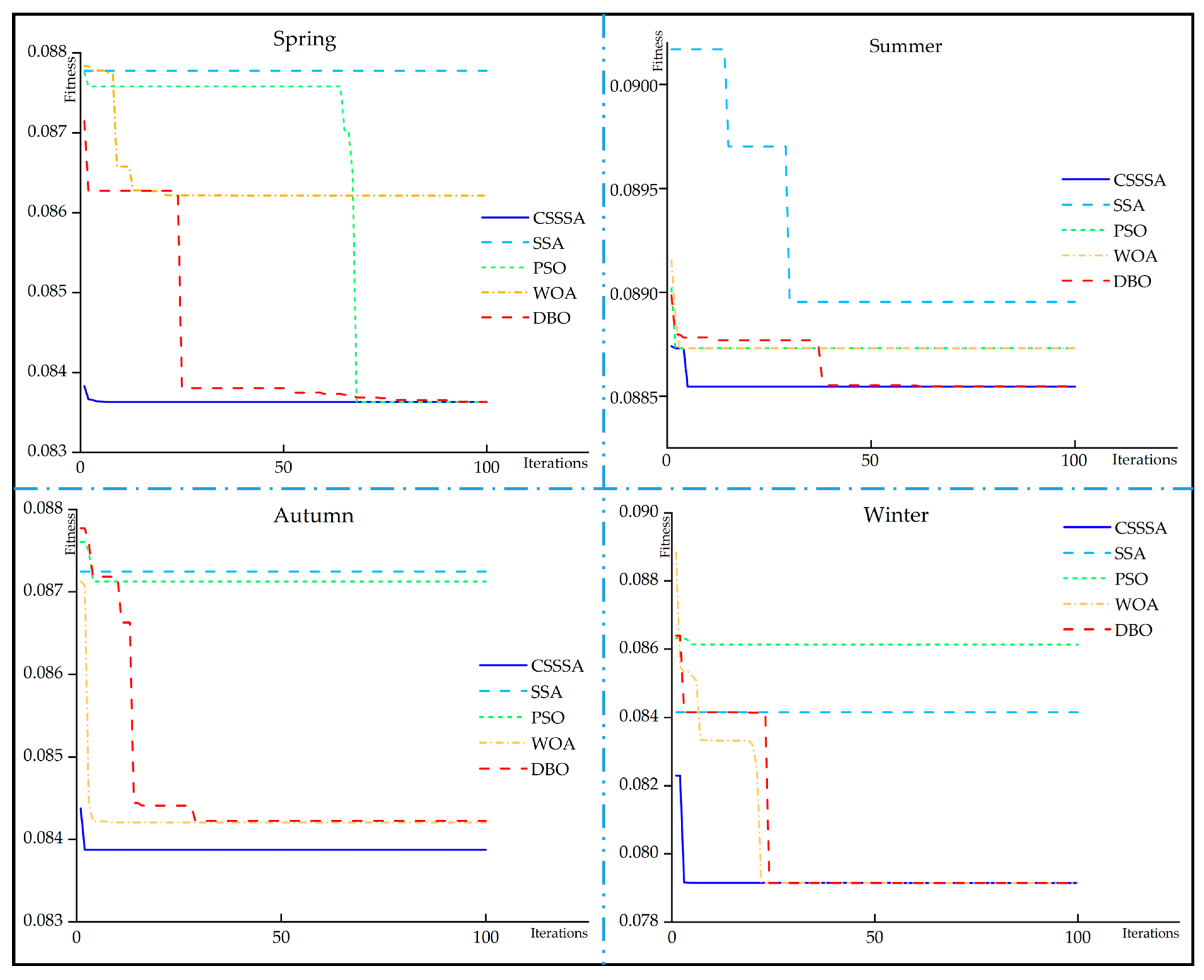
3.4.1. Comparative Results of CSSSA with Different Intelligent Algorithms

The core objective of Experiment 1 was to validate the effectiveness of CSSSA in optimizing the parameter selection for VMD. VMD is a powerful signal processing technique, but its performance is highly dependent on the selection of the penalty factor α and the number of decomposition layers, K. Improper parameter selection may lead to mode aliasing or the introduction of noise, affecting the decomposition effect. Traditional parameter selection methods, such as the center-frequency observation method, are effective to a certain extent, but the process is cumbersome and time-consuming, making it difficult to adapt to rapidly changing signal environments.

To address this issue, the CSSSA was used in this experiment and compared in detail with four other intelligent optimization algorithms (the SSA, PSO, WOA, and DBO). The experimental design covered four different seasons (spring, summer, fall, and winter) to simulate different signal environments. Each algorithm was performed for 100 iterations, and the optimal fitness values after each iteration were recorded. The effectiveness of each algorithm in optimizing the VMD parameters was evaluated by comparing the convergence speeds of the different algorithms and the final optimal solutions achieved. Figure 7 presents the convergence curves of different optimization algorithms across the four seasons, illustrating the differences in convergence speed and performance.

In the experiments, the CSSSA reached the optimal solution significantly faster than the SSA, PSO, WOA, and DBO, which required more iterations to approach the optimal solution. In all seasonal scenarios, the CSSSA consistently outperformed the other algorithms.

Additionally,

Table 4. A comparison of the prediction performance of different optimization algorithms for the same model across scenarios of the four seasons.

Model		Spring			Summer			Autumn			Winter
		RMSE	MAE	R2	RMSE	MAE	R2	RMSE	MAE	R2	RMSE	MAE	R2
CECSVB-LSTM	5 min	0.0992	0.0768	0.9965	0.0993	0.0641	0.9952	0.1309	0.0849	0.9927	0.0821	0.0706	0.9976
	10 min	0.1652	0.1179	0.9903	0.1770	0.1095	0.9850	0.1466	0.0969	0.9909	0.1110	0.0937	0.9957
CEEMDAN-SSA -VMD-BILSTM	5 min	0.5734	0.3468	0.8997	0.5231	0.3014	0.8830	0.3316	0.2794	0.9536	0.2494	0.2096	0.9784
	10 min	0.6461	0.3977	0.8728	0.6128	0.3708	0.8396	0.4707	0.4058	0.9067	0.3583	0.3039	0.9556
CEEMDAN-WOA -VMD-BILSTM	5 min	0.5409	0.2972	0.9099	0.4543	0.2545	0.9116	0.2839	0.2337	0.9655	0.4156	0.3732	0.9403
	10 min	0.6580	0.3799	0.8666	0.4866	0.2900	0.8986	0.4127	0.3455	0.9273	0.4604	0.3865	0.9268
CEEMDAN-PSO -VMD-BILSTM	5 min	0.5546	0.3201	0.9051	0.4757	0.2498	0.9033	0.2211	0.1766	0.9794	0.2702	0.2325	0.9746
	10 min	0.6583	0.4035	0.8661	0.5242	0.2999	0.8828	0.3078	0.2473	0.9602	0.3551	0.3084	0.9562
CEEMDAN-DBO -VMD-BILSTM	5 min	0.5448	0.3085	0.9081	0.5030	0.2495	0.8921	0.2620	0.2278	0.9708	0.2470	0.2199	0.9788
	10 min	0.6550	0.4020	0.8669	0.6133	0.3223	0.8403	0.3953	0.3405	0.9338	0.2599	0.2265	0.9766

shows the results of the comparison of the prediction performance of different optimization algorithms in the spring, summer, autumn, and winter scenarios. In the spring and summer scenarios, the CSSSA achieves RMSE values of 0.0992 kW and 0.0993 kW at 5 min steps, MAE values of 0.0768 kW and 0.0641 kW, and R² values close to 1, specifically 0.9965 and 0.9952, respectively. In the fall and winter scenarios, the CSSSA also performs well, with RMSE values of 0.1309 kW and 0.0821 kW at 5 min steps and MAE values of 0.0849 kW and 0.0706 kW. The R² values are 0.9927 and 0.9976. In contrast, other optimization algorithms, such as the SSA, WOA, PSO, and DBO, do not perform as well as the CSSSA in all seasonal scenarios, especially at the 10 min step, where the RMSE and MAE values of these algorithms are significantly higher than those of the CSSSA, and the R² values are also relatively low.

In summary, through the comparison experiments between the CSSSA and the other four intelligent optimization algorithms (the SSA, PSO, WOA, and DBO) under four seasonal scenarios, namely, spring, summer, autumn, and winter, we verified the excellent performance of the CSSSA in optimizing the VMD parameter selection. The CSSSA is not only better than the other algorithms in terms of convergence speed but also displays a better adaptation value in the final performance, indicating its remarkable efficiency and accuracy in optimizing the key parameters of VMD. The experimental results consistently show that the CSSSA is able to reach the optimal solution quickly and has a high prediction accuracy, with an R² value close to 1, which significantly improves the VMD decomposition. Therefore, the CSSSA can effectively overcome the limitations of traditional parameter selection methods, and its excellent optimization ability makes it the preferred algorithm for optimizing VMD parameters.

3.4.2. Ablation Study

To systematically evaluate the performance of the CECSVB-LSTM model in the short-term forecasting of PV power generation and assess the contribution of each component, an ablation experiment was designed for Experiment 2. This experiment compared the full model (CECSVB-LSTM) with partial models (including CEEMDAN-VMD-BILSTM, VMD-BILSTM, CEEMDAN-BILSTM, and BILSTM alone) across different seasons (spring, summer, autumn, and winter) and forecasting step sizes (5 min and 10 min). The prediction performance was evaluated in terms of root mean square error (RMSE), mean absolute error (MAE), and the coefficient of determination (R²), as shown in

Table 5. Results of model ablation experiments across scenarios of four seasons.

Model		Spring			Summer			Autumn			Winter
		RMSE	MAE	R2	RMSE	MAE	R2	RMSE	MAE	R2	RMSE	MAE	R2
CECSVB-LSTM	5 min	0.0992	0.0768	0.9965	0.0993	0.0641	0.9952	0.1309	0.0849	0.9927	0.0821	0.0706	0.9976
	10 min	0.1652	0.1179	0.9903	0.1770	0.1095	0.9850	0.1466	0.0969	0.9909	0.1110	0.0937	0.9957
CEEMDAN-VMD-BILSTM	5 min	0.1772	0.1044	0.9887	0.1605	0.1214	0.9846	0.1693	0.1219	0.9878	0.1764	0.1536	0.9894
	10 min	0.3108	0.1882	0.9653	0.2374	0.1788	0.9663	0.2383	0.1732	0.9760	0.2034	0.1811	0.9859
VMD-BILSTM	5 min	0.2541	0.1935	0.9761	0.2433	0.2058	0.9675	0.2489	0.2143	0.9734	0.2931	0.2547	0.9704
	10 min	0.3156	0.2388	0.9630	0.2865	0.2494	0.9550	0.2931	0.2560	0.9631	0.3775	0.3268	0.9508
CEEMDAN-BILSTM	5 min	0.2923	0.1698	0.9715	0.2661	0.1969	0.9678	0.2183	0.1736	0.9798	0.2670	0.2379	0.9757
	10 min	0.3454	0.1960	0.9602	0.3211	0.2411	0.9531	0.2867	0.2332	0.9652	0.3112	0.2789	0.9670
BILSTM	5 min	0.5157	0.2987	0.9117	0.3920	0.2264	0.9302	0.4296	0.3563	0.9221	0.4125	0.3355	0.9421
	10 min	0.6400	0.3658	0.8639	0.4568	0.2654	0.9052	0.4783	0.4045	0.9034	0.4328	0.3749	0.9362

.

The experimental results indicate that the full model CECSVB-LSTM significantly outperforms the other partial models in terms of prediction performance across all seasons. The RMSE and MAE values of the full model are significantly lower than those of the other models in both time steps of spring, summer, autumn, and winter, indicating smaller prediction errors. For instance, at the 5 min time step in spring, the RMSE of the full model is 0.0992 kW and the MAE is 0.0768 kW, while the RMSE of the model using only BILSTM is 0.5157 kW and the MAE is 0.2987 kW. In terms of the R² metrics, the values of the full model are close to 0.999 in all seasons, indicating that its predictions are highly consistent with the actual observations, while the R² values of the other partial models are significantly lower.

Additionally, the effectiveness of the CSSSA in optimizing VMD parameters can be clearly seen by comparing the results of CECSVB-LSTM and CEEMDAN-VMD-BILSTM. For example, in the autumn 5 min scenario, the RMSE of the complete model is 0.1309 kW, while the RMSE of the model without the CSSSA is 0.1693 kW, indicating that the CSSSA significantly improves the decomposition effect of VMD, thereby enhancing prediction accuracy.

In summary, the model proposed in this paper shows superior performance in experiments across different seasons, especially in spring and winter, and its prediction accuracy and robustness are further verified. Despite the more complicated weather conditions in summer, the model still performs better than some other models in all seasons. These results indicate that the CECSVB-LSTM model has significant advantages in dealing with the complexity and volatility of PV power generation data, and the synergistic effect of the components provides strong support for improving prediction accuracy and reliability.

3.4.3. Traditional Single-Model Comparison Experiment

In the single-model comparison experiments, several representative models, namely, the BP neural network, extreme learning machine (ELM), the bidirectional long short-term memory (BILSTM) network, and the Bidirectional Gated Recurrent Unit (BIGRU), are selected for comparison in this paper. As a classical feed-forward neural network, the BP neural network is widely used in regression and classification tasks. It is selected as a comparison model to evaluate the performance of the proposed model under the traditional neural network architecture and verify the superiority of the model in performing the PV power generation forecasting task. ELM is a fast learning algorithm for single hidden layer feed-forward neural networks, characterized by fast training speed and good generalization performance. By comparing it with ELM, the advantages of the proposed model in forecasting complex time series can be demonstrated, especially in handling the nonlinearities and volatility of PV power generation data. BILSTM, as a variant of LSTM, is able to capture both past and future information of time series data. By selecting BILSTM as a comparison model, the effectiveness of the proposed model in utilizing bidirectional temporal dependencies can be verified. BIGRU is a bidirectional version of GRU with a similar structure and functions. By comparing with BIGRU, the proposed model can further evaluate the performance differences under different bidirectional recurrent neural network architectures and verify the applicability and effectiveness of the model in PV power forecasting.

In Experiment 3, we validated the performance of the proposed CEEMDAN-CSSSA-VMD-BILSTM model in the PV power forecasting task through comparative experiments and performed detailed performance comparisons with other single models (the BP neural network, ELM, BILSTM, and BIGRU). The evaluation metrics included RMSE, MAE, and R². As shown in

Table 6. A comparison of the prediction performance between the proposed model and single models across scenarios of the four seasons.

Model		Spring			Summer			Autumn			Winter
		RMSE	MAE	R2	RMSE	MAE	R2	RMSE	MAE	R2	RMSE	MAE	R2
CECSVB-LSTM	5 min	0.0992	0.0768	0.9965	0.0993	0.0641	0.9952	0.1309	0.0849	0.9927	0.0821	0.0706	0.9976
	10 min	0.1652	0.1179	0.9903	0.1770	0.1095	0.9850	0.1466	0.0969	0.9909	0.1110	0.0937	0.9957
BP	5 min	0.5068	0.2528	0.9146	0.3781	0.1700	0.9350	0.3635	0.2967	0.9442	0.4007	0.3541	0.9454
	10 min	0.6402	0.3648	0.8635	0.4479	0.2050	0.9086	0.3853	0.3194	0.9373	0.4201	0.3675	0.9399
ELM	5 min	0.6145	0.3811	0.8746	0.5018	0.3327	0.8856	0.2768	0.2011	0.9676	0.1865	0.1421	0.9881
	10 min	0.7263	0.4796	0.8248	0.5709	0.4095	0.8519	0.3251	0.2532	0.9554	0.2072	0.1588	0.9853
BILSTM	5 min	0.5157	0.2987	0.9117	0.3920	0.2264	0.9302	0.4296	0.3563	0.9221	0.4125	0.3355	0.9421
	10 min	0.6400	0.3658	0.8639	0.4568	0.2654	0.9052	0.4783	0.4045	0.9034	0.4328	0.3749	0.9362
BIGRU	5 min	0.5377	0.3001	0.9040	0.3981	0.2469	0.9280	0.1899	0.1380	0.9847	0.3222	0.2799	0.9646
	10 min	0.6613	0.3844	0.8548	0.4987	0.3385	0.8870	0.2420	0.1818	0.9752	0.4322	0.3705	0.9364

and Figure 8, the experimental results demonstrate that the proposed model exhibits superior performance in predicting 5 min and 10 min steps across spring, summer, autumn, and winter. Specifically, the proposed model significantly outperforms other single models in terms of RMSE, MAE, and R² in spring and winter, performs well in all evaluation metrics in summer despite the complex weather conditions, and achieves the best performance in terms of RMSE and MAE in autumn, with R² close to 1.

In contrast, traditional single models (e.g., the BP neural network and ELM) perform poorly in dealing with the complexity and volatility of PV power generation data, especially under complex weather conditions, where their prediction accuracy and robustness are obviously insufficient. Although bidirectional recurrent neural networks (BILSTM and BIGRU) have certain advantages in time series prediction, they still have limitations in utilizing bidirectional time dependencies. Our experimental results verify the significant advantages of the CEEMDAN-CSSSA-VMD-BILSTM model in handling the complexity and volatility of PV power generation data. The joint action of its components significantly improves the accuracy and reliability of the prediction, demonstrating the good applicability and validity of this model in PV power generation prediction tasks.

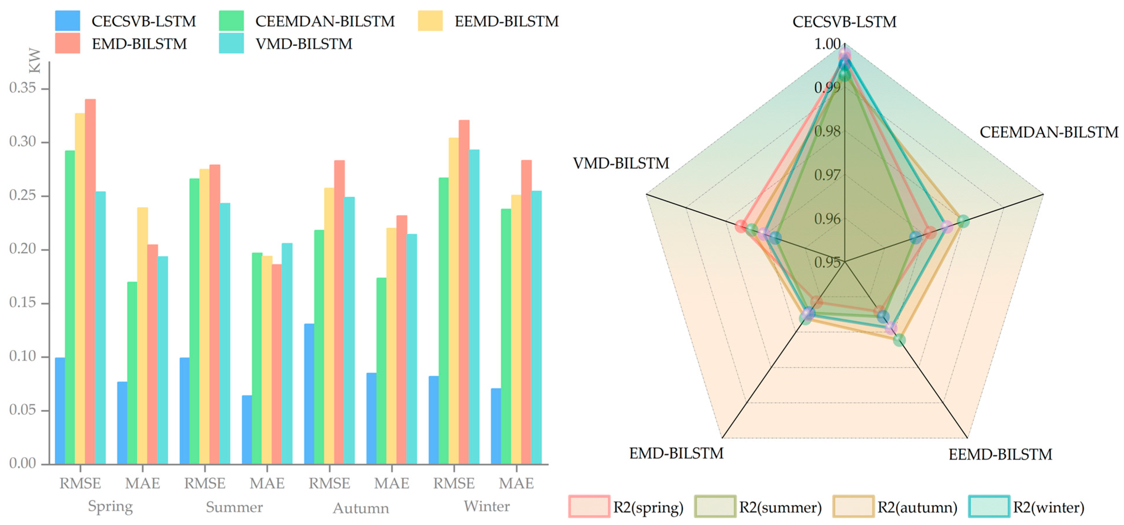
3.4.4. Comparison Experiment of Different Signal Decomposition Methods

In Experiment 4, we validated the advantages of the proposed CECSVB-LSTM model as a dual decomposition method for PV power generation prediction through comparative experiments. The purpose of the experiment was to demonstrate the superiority of the combination of CEEMDAN and CSSSA-VMD in terms of feature separation and prediction accuracy. The comparisons included CEEMDAN-BILSTM, EMD-BILSTM, EEMD-BILSTM, and VMD-BILSTM. The experiments were designed to test the effects of different decomposition algorithms under the same BILSTM framework, with evaluation metrics including RMSE, MAE, and R². The experimental data covered four seasons: spring, summer, autumn, and winter, with prediction steps of 5 min and 10 min.

As shown in

Table 7. A comparison of the prediction performance between the proposed model and different signal decomposition methods across scenarios of the four seasons.

Model		Spring			Summer			Autumn			Winter
		RMSE	MAE	R2	RMSE	MAE	R2	RMSE	MAE	R2	RMSE	MAE	R2
CECSVB-LSTM	5 min	0.0992	0.0768	0.9965	0.0993	0.0641	0.9952	0.1309	0.0849	0.9927	0.0821	0.0706	0.9976
	10 min	0.1652	0.1179	0.9903	0.1770	0.1095	0.9850	0.1466	0.0969	0.9909	0.1110	0.0937	0.9957
CEEMDAN-BILSTM	5 min	0.2923	0.1698	0.9715	0.2661	0.1969	0.9678	0.2183	0.1736	0.9798	0.2670	0.2379	0.9757
	10 min	0.3454	0.1960	0.9602	0.3211	0.2411	0.9531	0.2867	0.2332	0.9652	0.3112	0.2789	0.9670
EEMD-BILSTM	5 min	0.3270	0.2393	0.9642	0.2751	0.1941	0.9656	0.2574	0.2201	0.9722	0.3040	0.2509	0.9688
	10 min	0.4058	0.2794	0.9449	0.3253	0.2219	0.9518	0.3198	0.2629	0.9571	0.3769	0.3158	0.9521
EMD-BILSTM	5 min	0.3402	0.2046	0.9615	0.2790	0.1862	0.9645	0.2832	0.2318	0.9661	0.3207	0.2833	0.9650
	10 min	0.4393	0.2046	0.9358	0.3659	0.2622	0.9388	0.3311	0.2555	0.9536	0.4491	0.2833	0.9314
VMD-BILSTM	5 min	0.2541	0.1935	0.9761	0.2433	0.2058	0.9675	0.2489	0.2143	0.9734	0.2931	0.2547	0.9704
	10 min	0.3156	0.2388	0.9630	0.2865	0.2494	0.9550	0.2931	0.2560	0.9631	0.3775	0.3268	0.9508

and Figure 9, the experimental results indicate that the CECSVB-LSTM model outperforms the combined models of other single decomposition methods in all assessment metrics. The model performs best on the RMSE and MAE metrics in spring and winter, with R² metrics close to 1, showing its significant advantage in dealing with data complexity and volatility. In summer, the proposed model maintains a low prediction error despite the complex weather conditions, while in autumn, it also performs well on the RMSE and MAE metrics, with an R² metric close to 1. In contrast, traditional single decomposition methods, such as EEMD and EMD, have higher errors under complex weather conditions. VMD is sensitive to the number of modes and has unstable initialization when dealing with the non-stationarity of PV power generation data, limiting its performance in complex PV generation data. While CEEMDAN-BILSTM performs better in some metrics, its overall performance is not as good as the proposed model. These results validate the advantages of the CEEMDAN-CSSSA-VMD dual decomposition method in refining feature separation and reducing prediction errors, demonstrating its applicability and effectiveness in PV power generation prediction tasks.

4. Conclusions

Aiming at the key issues of data nonlinearity, intermittency, and model parameter optimization in the short-term prediction of PV power generation, this paper proposes a hybrid prediction model, CECSVB-LSTM, which combines dual decomposition techniques and improved intelligent algorithms. The model preliminarily decomposes the PV power series using CEEMDAN to capture complex nonlinear features and optimizes the key parameters of the variational mode decomposition (VMD) using the Sparrow Search Algorithm (CSSSA), which integrates Circle chaos mapping and Sine Cosine Algorithms, to achieve fine separation of high-frequency components. A multivariate input prediction framework was constructed by leveraging the BiLSTM network’s ability to capture time series dependencies in both directions. The experimental results show that the proposed model performs well on measured data from Australian solar power plants: compared to traditional single models, such as BP and ELM, the coefficient of determination R² is improved by more than 7.98%, and the root mean square error (RMSE) and mean absolute error (MAE) are reduced by 60% and 55%, respectively. Compared to combined models using single decomposition methods, the non-stationary signal processing error is reduced by more than 30%, significantly improving feature extraction efficiency and prediction accuracy. Under different seasons and prediction steps, the model maintains stable and high accuracy, with an R² close to 0.99, verifying the synergistic advantage of the dual decomposition strategy and the intelligent optimization algorithm. While the CECSVB-LSTM model exhibits remarkable predictive performance. However, two primary limitations should be acknowledged. Firstly, the multi-stage decomposition approach (CEEMDAN combined with VMD) and the BiLSTM structure result in relatively high computational complexity. This may constrain its applicability in real-time scenarios with stringent latency constraints, such as ultra-fast grid dispatching. Secondly, the model validation predominantly utilizes data from a single solar plant in Australia. Although the dataset encompasses four seasons, it lacks sufficient representation of diverse global climatic regions (e.g., tropical and desert climates) and extreme weather events (e.g., typhoons). This could introduce uncertainties when deploying the model on a broader scale. In the future, research will further incorporate statistical methods such as 95% confidence intervals and hypothesis testing (e.g., t-tests) to evaluate model performance differences, integrate numerical weather prediction, satellite remote sensing, and other multi-source data to improve generalization ability, develop dynamic adaptive mechanisms to cope with equipment aging and sudden environmental changes, and provide more accurate technical support for smart grid scheduling and efficient consumption of renewable energy.

References

1. Sabadus, A.; Blaga, R.; Hategan, S.M.; Calinoiu, D.; Paulescu, E.; Mares, O.; Boata, R.; Stefu, N.; Paulescu, M.; Badescu, V. A cross-sectional survey of deterministic PV power forecasting: Progress and limitations in current approaches. Renew. Energy 2024, 226, 120385. [Google Scholar] [CrossRef]
2. Jebli, I.; Belouadha, F.Z.; Kabbaj, M.I.; Tilioua, A. Prediction of solar energy guided by pearson correlation using machine learning. Energy 2021, 224, 120109. [Google Scholar] [CrossRef]
3. Kim, G.G.; Lee, W.; Bhang, B.G.; Choi, J.H.; Ahn, H.K. Fault Detection for Photovoltaic Systems Using Multivariate Analysis With Electrical and Environmental Variables. IEEE J. Photovolt. 2021, 11, 202–212. [Google Scholar] [CrossRef]
4. Zhu, T.; Li, Q.; Yu, A. Analysis of the solar spectrum allocation in a spectral-splitting photovoltaic-thermochemical hybrid system. Sol. Energy 2022, 232, 63–72. [Google Scholar] [CrossRef]
5. Zhang, H.C.; Zhu, T.T. Stacking Model for Photovoltaic-Power-Generation Prediction. Sustainability 2022, 14, 5669. [Google Scholar] [CrossRef]
6. Rajagukguk, R.A.; Ramadhan, R.A.A.; Lee, H.J. A Review on Deep Learning Models for Forecasting Time Series Data of Solar Irradiance and Photovoltaic Power. Energies 2020, 13, 6623. [Google Scholar] [CrossRef]
7. Boubakr, G.; Gu, F.S.; Farhan, L.; Ball, A. Enhancing Virtual Real-Time Monitoring of Photovoltaic Power Systems Based on the Internet of Things. Electronics 2022, 11, 2469. [Google Scholar] [CrossRef]
8. Rodríguez, F.; Galarza, A.; Vasquez, J.C.; Guerrero, J.M. Using deep learning and meteorological parameters to forecast the photovoltaic generators intra-hour output power interval for smart grid control. Energy 2022, 239, 122116. [Google Scholar] [CrossRef]
9. Ye, W.J.; Yang, D.M.; Tang, C.H.; Wang, W.; Liu, G. Combined Prediction of Wind Power in Extreme Weather Based on Time Series Adversarial Generation Networks. IEEE Access 2024, 12, 102660–102669. [Google Scholar] [CrossRef]
10. Mayer, M.J.; Gróf, G. Extensive comparison of physical models for photovoltaic power forecasting. Appl. Energy 2021, 283, 116239. [Google Scholar] [CrossRef]
11. Ahmed, R.; Sreeram; Mishra, Y.; Arif, M.D. A review and evaluation of the state-of-the-art in PV solar power forecasting: Techniques and optimization. Renew. Sustain. Energy Rev. 2020, 124, 109792. [Google Scholar] [CrossRef]
12. Nam, S.; Hur, J. A hybrid spatio-temporal forecasting of solar generating resources for grid integration. Energy 2019, 177, 503–510. [Google Scholar] [CrossRef]
13. Liu, L.S.; Guo, K.Q.; Chen, J.; Guo, L.; Ke, C.Y.; Liang, J.R.; He, D.W. A Photovoltaic Power Prediction Approach Based on Data Decomposition and Stacked Deep Learning Model. Electronics 2023, 12, 2764. [Google Scholar] [CrossRef]
14. Pan, M.Z.; Li, C.; Gao, R.; Huang, Y.T.; You, H.; Gu, T.S.; Qin, F.R. Photovoltaic power forecasting based on a support vector machine with improved ant colony optimization. J. Clean. Prod. 2020, 277, 123948. [Google Scholar] [CrossRef]
15. Zhou, Y.; Zhou, N.R.; Gong, L.H.; Jiang, M.L. Prediction of photovoltaic power output based on similar day analysis, genetic algorithm and extreme learning machine. Energy 2020, 204, 117894. [Google Scholar] [CrossRef]
16. Behera, M.K.; Majumder, I.; Nayak, N. Solar photovoltaic power forecasting using optimized modified extreme learning machine technique. Eng. Sci. Technol. Int. J. 2018, 21, 428–438. [Google Scholar] [CrossRef]
17. Heng, S.Y.; Ridwan, W.M.; Kumar, P.; Ahmed, A.N.; Fai, C.M.; Birima, A.H.; El-Shafie, A. Artificial neural network model with different backpropagation algorithms and meteorological data for solar radiation prediction. Sci. Rep. 2022, 12, 10457. [Google Scholar] [CrossRef]
18. Zheng, J.Q.; Zhang, H.R.; Dai, Y.H.; Wang, B.H.; Zheng, T.C.; Liao, Q.; Liang, Y.T.; Zhang, F.W.; Song, X. Time series prediction for output of multi-region solar power plants. Appl. Energy 2020, 257, 114001. [Google Scholar] [CrossRef]
19. Mellit, A.; Pavan, A.M.; Lughi, V. Deep learning neural networks for short-term photovoltaic power forecasting. Renew. Energy 2021, 172, 276–288. [Google Scholar] [CrossRef]
20. Zhou, Y.; Liu, Y.F.; Wang, D.J.; Liu, X.J.; Wang, Y.Y. A review on global solar radiation prediction with machine learning models in a comprehensive perspective. Energy Convers. Manag. 2021, 235, 113960. [Google Scholar] [CrossRef]
21. Zhu, H.L.; Li, X.; Sun, Q.; Nie, L.; Yao, J.X.; Zhao, G. A Power Prediction Method for Photovoltaic Power Plant Based on Wavelet Decomposition and Artificial Neural Networks. Energies 2016, 9, 11. [Google Scholar] [CrossRef]
22. Liu, H.; Mi, X.W.; Li, Y.F. Wind speed forecasting method based on deep learning strategy using empirical wavelet transform, long short term memory neural network and Elman neural network. Energy Convers. Manag. 2018, 156, 498–514. [Google Scholar] [CrossRef]
23. Yang, X.Y.; Yang, L.; Li, Y.K.; Zhao, Z.Y.; Zhang, Y.F. A new method of photovoltaic clusters power prediction based on Informer considering time-frequency analysis and convergence effect. Electr. Power Syst. Res. 2025, 238, 111049. [Google Scholar] [CrossRef]
24. Wen, Y.; Pan, S.; Li, X.X.; Li, Z.B. Highly fluctuating short-term load forecasting based on improved secondary decomposition and optimized VMD. Sustain. Energy Grids Netw. 2024, 37, 101270. [Google Scholar] [CrossRef]
25. Chen, J.Y.; Liu, L.S.; Guo, K.Q.; Liu, S.R.; He, D.W. Short-Term Electricity Load Forecasting Based on Improved Data Decomposition and Hybrid Deep-Learning Models. Appl. Sci. 2024, 14, 5966. [Google Scholar] [CrossRef]
26. Wang, S.C.; Huang, Y. Spatio-temporal photovoltaic prediction via a convolutional based hybrid network. Comput. Electr. Eng. 2025, 123, 110021. [Google Scholar] [CrossRef]
27. Wang, Y.; Bi, Y.; Guo, Y.; Liu, X.L.; Sun, W.Q.; Yu, Y.; Yang, J.Q. A Wind and Solar Power Prediction Method Based on Temporal Convolutional Network-Attention-Long Short-Term Memory Transfer Learning and Sensitive Meteorological Features. Appl. Sci. 2025, 15, 1636. [Google Scholar] [CrossRef]
28. Zhang, J.L.; Tan, Z.F.; Wei, Y.M. An adaptive hybrid model for day-ahead photovoltaic output power prediction. J. Clean. Prod. 2020, 244, 118858. [Google Scholar] [CrossRef]
29. Chen, X.; Ding, K.; Zhang, J.W.; Han, W.; Liu, Y.J.; Yang, Z.N.; Weng, S. Online prediction of ultra-short-term photovoltaic power using chaotic characteristic analysis, improved PSO and KELM. Energy 2022, 248, 123574. [Google Scholar] [CrossRef]
30. An, G.Q.; Jiang, Z.Y.; Chen, L.B.; Cao, X.; Li, Z.; Zhao, Y.Y.; Sun, H.X. Ultra Short-Term Wind Power Forecasting Based on Sparrow Search Algorithm Optimization Deep Extreme Learning Machine. Sustainability 2021, 13, 10453. [Google Scholar] [CrossRef]
31. Jia, P.Y.; Zhang, H.B.; Liu, X.M.; Gong, X.F. Short-Term Photovoltaic Power Forecasting Based on VMD and ISSA-GRU. IEEE Access 2021, 9, 105939–105950. [Google Scholar] [CrossRef]
32. Wang, L.; Liu, Y.; Li, T.; Xie, X.; Chang, C. Short-term PV power prediction based on optimized VMD and LSTM. IEEE Access 2020, 8, 165849–165862. [Google Scholar] [CrossRef]
33. Xue, J.K.; Shen, B.; Pan, A.Q. A hierarchical sparrow search algorithm to solve numerical optimization and estimate parameters of carbon fiber drawing process. Artif. Intell. Rev. 2023, 56, 1113–1148. [Google Scholar] [CrossRef]
34. Zhang, X.Q.; Zheng, Z.W. A Novel Groundwater Burial Depth Prediction Model Based on Two-Stage Modal Decomposition and Deep Learning. Int. J. Environ. Res. Public Health 2023, 20, 345. [Google Scholar] [CrossRef] [PubMed]
35. Sepulveda-Oviedo, E.H. Impact of environmental factors on photovoltaic system performance degradation. Energy Strategy Rev. 2025, 59, 101682. [Google Scholar] [CrossRef]
36. Gueymard, C.A. A review of validation methodologies and statistical performance indicators for modeled solar radiation data: Towards a better bankability of solar projects. Renew. Sustain. Energy Rev. 2014, 39, 1024–1034. [Google Scholar] [CrossRef]
Figure 1. Chaotic value distribution of Circle map: pre-improvement (a) and post-improvement (b), showing optimized uniformity.
Energies 18 03136 g001
Figure 2. LSTM structure.
Energies 18 03136 g002
Figure 3. BILSTM structure.
Energies 18 03136 g003
Figure 4. Flowchart of CECSVB-LSTM.
Energies 18 03136 g004
Figure 5. Signal decomposition and processing steps of the proposed model: (a) initial decomposition of photovoltaic power time series based on CEEMDAN; (b) clustering classification of IMFs based on K-means; (c) secondary decomposition of high-frequency signals based on VMD.
Energies 18 03136 g005
Figure 6. Curve chart of photovoltaic power generation varying with time.
Energies 18 03136 g006
Figure 7. Comparative convergence curves of different optimization algorithms.
Energies 18 03136 g007
Figure 8. Comparison of prediction performance among multiple models across four seasons.
Energies 18 03136 g008
Figure 9. Comparison of prediction performance of different signal decomposition methods for PV power generation.
Energies 18 03136 g009