1. Introduction
With the active promotion of the offshore wind power industry in China, by 2023, China had secured the leading position in the global offshore wind power market. Nevertheless, the output characteristics of offshore wind power generation show significant volatility, which undoubtedly increases the risk of instability in its grid-connected operation [
1,
2]. In view of this, the National Development and Reform Commission (NDRC) issued the “Guiding Opinions on Encouraging renewable energy power generation Enterprises to Build or Purchase peak load Capacity to expand the scale of grid-connected operations” [
3]. This policy aims to ensure that new energy power companies have a sufficient proportion of energy storage systems to cope with unstable output situations [
4]. Electrochemical energy storage technology has become the preferred solution for the vast majority of offshore wind power enterprises due to its cost effectiveness, rapid deployment advantages [
5], and relatively unrestricted geographical conditions [
6,
7,
8,
9].
Domestic and foreign scholars have carried out in-depth research on the configuration of electrochemical energy storage in offshore wind farms. Paul et al. [
10] proposed a novel multi-objective optimization framework to determine the optimal capacity of battery energy storage systems (BESSs) in the collaborative operation of large offshore wind farms (OWFs) and BESSs, taking into account the battery cost and life, as well as the availability of wind turbines. Tian et al. [
11] used a hybrid hydrogen energy storage system to smooth the output volatility of offshore wind power and discussed the relationship between the abandoned air volume, volatility, and economy. The results show that the addition of hydrogen energy storage system will greatly reduce the economy of energy storage systems. Wu et al. [
12] proposed a voltage control method based on the reactive power coordination and electrochemical energy storage of wind farms, which can well improve the stability of the grid-connected voltage of offshore wind farms. Mokhtare et al. [
13] considered the rated capacity and rated power configuration of an optimal battery energy storage system that gives priority to meeting the grid-connected requirements of offshore wind farms in order to achieve the highest economy. Li et al. [
14] integrated a large-scale offshore wind power system, coupled thermal power station, electrochemical energy storage system, and floating photovoltaic system to improve the overall economy and system performance. Based on the configuration of battery energy storage in offshore wind power, supercapacitor energy storage was added to prevent the over-charge and over-discharge of the battery so as to improve the service life of the battery [
15]. Studies on the deployment of electrochemical energy storage in offshore wind farms have well revealed the help of electrochemical energy storage for the grid connection of offshore wind farms, but there are few studies on the relationship between the output power volatility and investment cost of offshore wind farms.
Most studies addressing both the volatility and investment cost in offshore wind power systems have investigated hybrid energy storage solutions. For example, Lu et al. [
16] combined lithium-ion batteries with supercapacitors and applied wavelet decomposition to allocate high-frequency fluctuations to supercapacitors and low-frequency variations to batteries. This hybrid configuration reduced the daily energy storage input costs by 2.79% and 3.84%, respectively, compared with standalone battery or supercapacitor schemes, while meeting volatility requirements. In another study, Lu et al. [
17] evaluated a 2 MW wind farm equipped with a hybrid storage system that comprised electrolytic cells, fuel cells, and supercapacitors; the optimization of this configuration achieved a 41.1% reduction in the annualized cost. Li et al. [
18] proposed an electric–hydrogen hybrid storage system controlled via deep reinforcement learning to coordinate the battery and hydrogen production unit operation. Their method reduced the average daily wind power fluctuation range from 20.11 MW to 5.74 MW—a 71.5% decrease—while enhancing the storage utilization efficiency. Chen et al. [
19] combined lithium-ion battery storage with expanded transmission capacity to improve the wind power utilization and lower the overall investment; they demonstrated that compared with merely upgrading the transmission infrastructure, adding appropriately sized storage could achieve equivalent consumption levels at a reduced cost. Most of these studies focused on the parameter changes of wind farms themselves, without considering the impact of energy storage on the policy changes of the electricity market and participation in real-time electricity trading.
This study combined the latest policies of China’s electricity market, introduced the spot trading model, proposed and compared three different schemes considering the investment cost and output power volatility of energy storage, considered them from the grid side and the power generation side, and used the change in SOC after configuring energy storage to evaluate the actual lifespan of the energy storage battery in this project. In order to improve the reliability of the calculation examples, this study conducted a comparative analysis using NSGA-II and the MOPSO algorithm, selected the better solutions of the two, and presented the optimal configuration with both the investment cost and power volatility under different circumstances.
3. Methods
In this study, Python 3.8 was adopted, and the capacity optimization of offshore wind power equipped with electrochemical energy storage was carried out by using NSGA-II through the imported SYS module. In this study, NSGA-II was used to optimize the capacity of offshore wind power equipped with electrochemical energy storage. Based on genetic algorithms, the algorithm significantly reduced the computational complexity and maintained population diversity through a fast non-dominated sorting process, density estimation (using crowding distances), and an explicit selection mechanism [
25]. In NSGA-II, the crowding distance was used to measure the distribution density of individuals in the objective space [
26]. For the middle individual, the crowding distance is the sum of the differences between the individual and the neighboring individuals in all objective functions. Specifically, for the
individual, the crowding distance is calculated as follows [
27]:
where
M is the number of objective functions;
is the value of individual
i on the
objective function; and
and
are the maximum and minimum values of this objective function in the population, respectively. The introduction of the crowding distance takes into account the distribution of individuals and avoids the selection of individuals too concentrated in some areas so as to maintain the diversity of the population and improve the search ability and convergence of the algorithm. Sun et al. enhanced NSGA-II to optimize the multi-objective configuration of wind and hydrogen systems, demonstrating that the total system cost was reduced by CNY 18 million through the introduction of an elite strategy [
28]. This study utilized NSGA-II to optimize the capacity of offshore wind power integrated with electrochemical energy storage. It thoroughly analyzed the performance data of offshore wind farms and preliminarily established a potential range for energy storage capacity, and thus, reduced the computational effort required in subsequent optimization steps. In this study, the energy storage power was randomly initialized within the range of 0 to 12 MW, and the rated capacity was randomly initialized within the range of 0 to 48 MWh. An initial population of 20 individuals was generated, with each individual representing a potential energy storage configuration. In each generation, 60 offspring were produced through genetic operations, and 20 individuals were selected to form the next generation to maintain a constant population size. The crossover and mutation probabilities were both set to 0.5, and the algorithm iterated for 300 generations. The simplified procedural steps are illustrated in
Figure 2 and described as follows:
Step 1: The relevant parameters of the offshore wind power plant were input, the feasible ranges for rated power and capacity of the energy storage system were defined, and these variables were encoded into two-dimensional individuals to form the initial population. Each individual was evaluated using the objective function and constraints to ensure compliance with initial conditions.
Step 2: Genetic operators were defined with crossover and mutation probabilities set at 0.5. Twenty energy storage configurations were randomly generated and their performances and feasibilities were evaluated.
Step 3: Evolutionary operations, including reproduction, evaluation, parent–offspring merging, and selection, were conducted over 300 generations to derive a convergent and diverse Pareto front.
Step 4: The optimal solutions were extracted by analyzing the 20 sets of rated power and capacity data, along with their corresponding objective values. Configurations that met the desired criteria were identified based on the relationship between the rated power and capacity, and the results were visualized.
4. Results
This study selected a 40 MW wind farm in Wan’an County composed of 16 wind turbines with a single-unit power of 2.5 MW as the research object. The output power data of the wind turbines of this wind farm throughout 2023 was selected as the reference for the energy storage configuration. In order to explore the relationship between the rated power and rated capacity of the energy storage configuration and the life of energy storage batteries, first, we selected the typical weeks when the proportion of wind power output time exceeds 80% for research according to Scheme 1 (the period from 9 to 15 December was selected for this study). The cost parameters utilized in this analysis are detailed in
Table 2. Given the significant regional variations in the electrochemical ESS disposal costs, this factor was excluded from the current calculation, which potentially led to a conservative estimate of the investment costs. The operational lifespan of the ESS was set at 25 years. Considering that the typical cycle life of electrochemical storage equipment was approximately 8000 cycles with a service life of around 10 years, it was anticipated that the battery system will require two replacements over the entire operational period. In this study, the volatility of the wind power output was analyzed by configuring an energy storage system (ESS) to align the instantaneous wind power output with the daily average power. The daily average power was calculated as the mean of 144 ten-minute interval power recordings per day. For the period from 9 to 15 December, the output power smoothness index
of the wind farm without the ESS configuration was calculated to be 27.23%. The reduction rate in the output power volatility
achieved through the ESS configuration was calculated as follows:
Figure 3 shows the Pareto frontier obtained by NSGA-II, which reflected the optimal allocation of the energy storage capacity and power under different cost constraints.
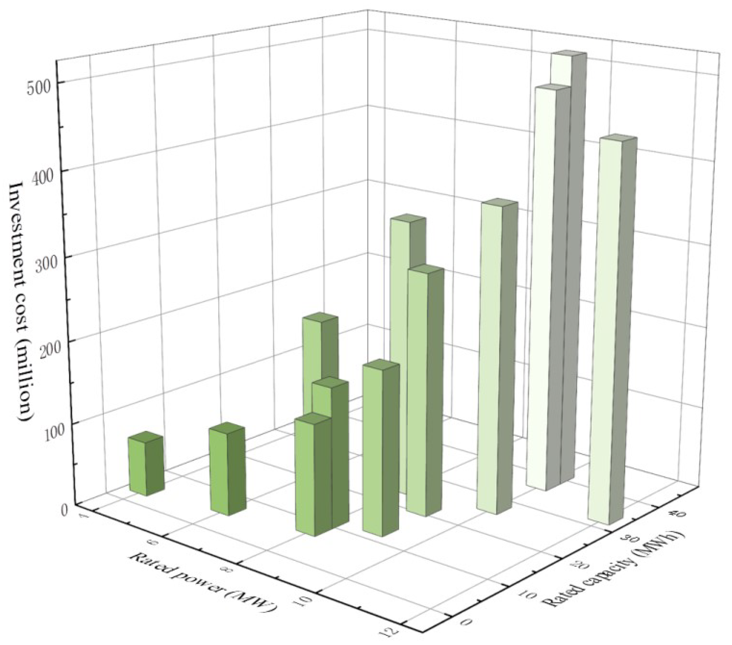
Figure 4 and
Figure 5 respectively show the impacts of changes in the rated power and rated capacity of energy storage system on the overall investment cost of the energy storage system and the output power fluctuation of offshore wind power after storage. In this study, the rated power variation range of the energy storage system was set at 10–30% of the rated power of wind farm. At the same time, the continuous working time of the energy storage was changed from 1 h to 4 h. Through the analysis, it is found that with the increase in the power and capacity of the energy storage system, the output power volatility of the wind farm after the configuration of the energy storage decreased from 22.48% to 18.63%, the volatility reduction rate increased from 5.29% to 21.18%, and the investment cost of the energy storage system increased from CNY 67.04 million to CNY 520.45 million. This trend suggests that in order to achieve better smoothing, more energy storage systems are needed to smooth out the wind power output fluctuations and reduce its instability. In addition, with the increase in cost, we observed that the overall smoothness of the output power curve after the allocation of wind power storage was significantly improved.
However, in the process of optimizing the configuration of the energy storage system by NSGA-II, the potential impacts of the rated power and rated capacity on the life of the energy storage battery must be carefully considered. Changes in these parameters will directly affect the SOC state of the battery at various points in time, thus having a decisive impact on its service life.
Table 3 shows the cycle times of the energy storage battery corresponding to each optimization solution on the Pareto front and its estimated life period, while
Figure 6 reflects the distribution of the Pareto front after the life correction. The analysis shows that in the case of a low-rated-power and low-rated-capacity configuration of the energy storage system, the charge and discharge frequency of the battery per unit time will increase and the depth of charge and discharge will be intensified, which will undoubtedly accelerate the aging process of the battery and greatly reduce its service life. As a result, the frequency of battery replacement will increase throughout the life cycle of the energy storage system, which will negatively affect the overall economic operating efficiency of the system. In order to quantify the specific effects of the rated power and rated capacity on the life of energy storage batteries, a multiple linear regression model was used for the fitting analysis. The model was able to establish the statistical correlation between the storage battery life
Y and its rated power
and rated capacity
:
When predicting the service life of the energy storage battery, the fitting degree
= 0.96965 shown by the multiple linear regression model indicates that the model had a high degree of agreement with the actual data, which provides strong confidence for our prediction. Through this model, we found that the service life of the energy storage battery was mainly affected by the rated capacity, and this impact showed a positive correlation. Specifically, when the rated capacity of the energy storage system was small, the actual cost was often higher than the expected cost simulated by NSGA-II. When the rated capacity was large, the actual cost could be lower than the cost of the algorithm simulation. This finding reveals that in the process of optimal allocation, relying only on the Pareto frontier obtained by NSGA-II may lead to a biased estimation of the economy. Therefore, in order to ensure an economic evaluation closer to the real situation, the Pareto frontier generated by NSGA-II must be modified based on the energy storage battery life. The Pareto frontier after the life correction is shown in
Figure 6, which provides us with a more accurate and practical decision basis. Through in-depth analysis and correction of the energy storage battery life, the impact of the rated capacity on the cost of the energy storage system could be more comprehensively understood.
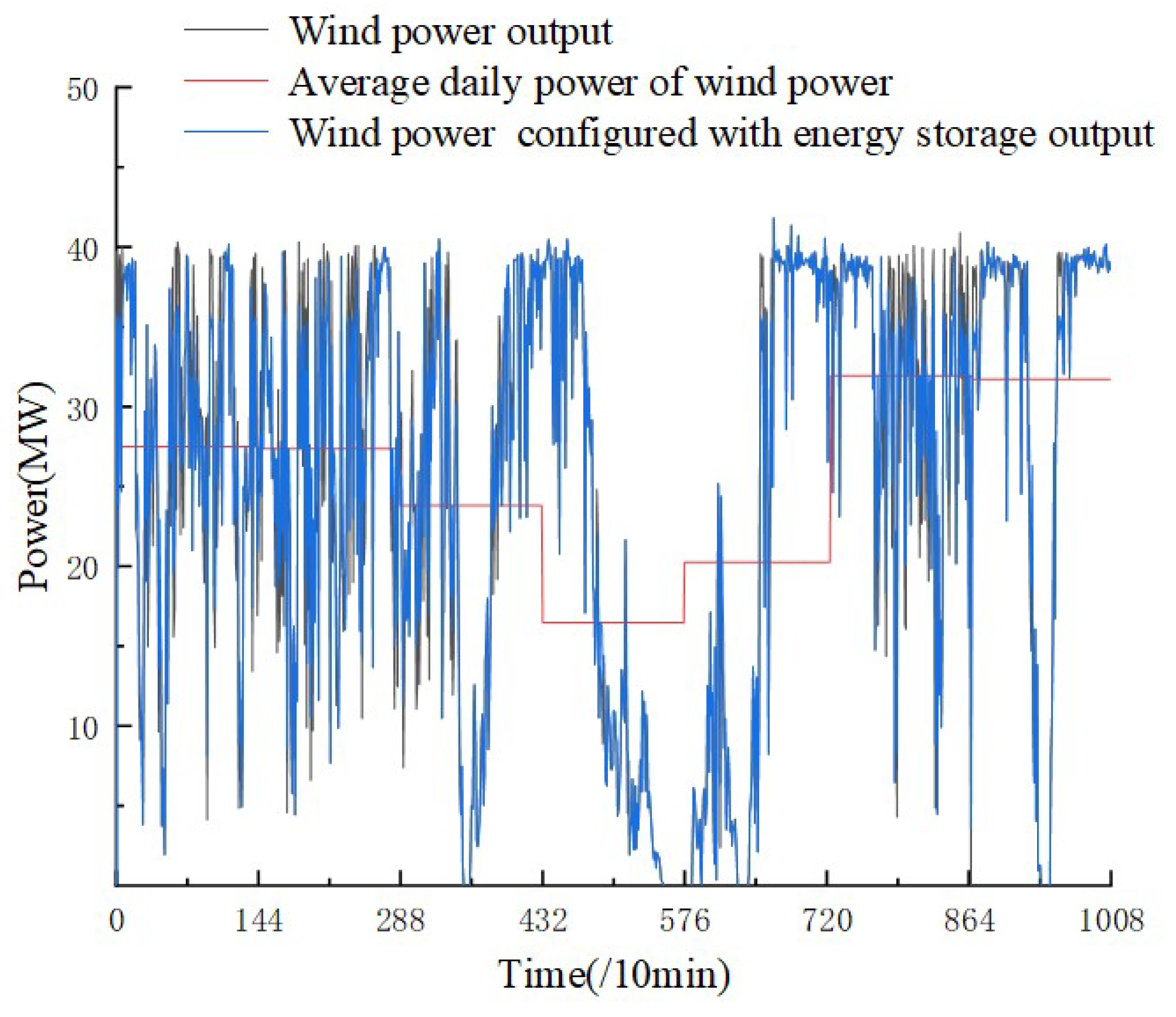
Figure 7 and
Figure 8 respectively show the comparison of the output power before and after the wind farm was configured with 10% energy storage and 25% energy storage. It can be clearly seen that the overall output curve was smoother when the wind farm was configured with a high proportion of energy storage.
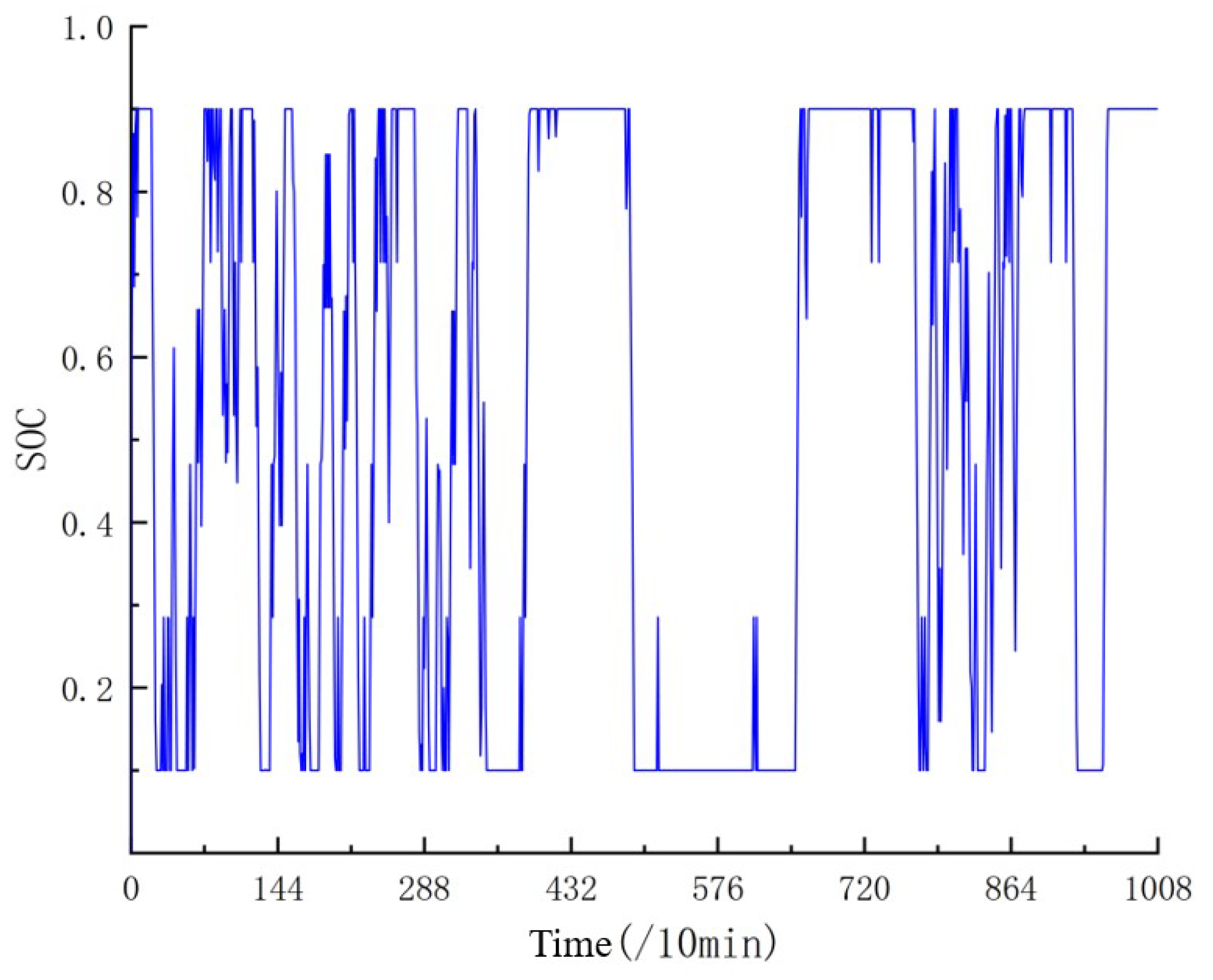
Figure 9 and
Figure 10 show the state charge (SOC) change curve of the energy storage system batteries with different proportions of energy storage, indicating that the SOC of the batteries was kept within a reasonable range during the entire operation cycle, thus ensuring the stable operation and efficient management of the energy storage system.
Due to significant seasonal variations in the wind speed, the power outputs of the wind turbines varied considerably throughout the year. As a result, an energy storage configuration based on a single week of data could not accurately represent the actual long-term demand of the wind farm. To address this limitation, the life correction method introduced in the previous section was applied to the full-year dataset, which enabled a comprehensive assessment of the annual energy storage configuration. The modified Pareto front obtained through this process is illustrated in
Figure 11. To evaluate and identify the optimal energy storage configuration, this study employed the multi-objective particle swarm optimization (MOPSO) algorithm as a benchmark against NSGA-II. The MOPSO parameter settings are listed in
Table 4, and the resulting Pareto front is depicted in
Figure 12. For a quantitative comparison of each algorithm’s trade-off performance, we introduce the metric
, which is defined as the incremental energy storage investment cost required to achieve a 1% reduction in the output volatility:
Table 5 reports the
values on the Pareto front produced by NSGA-II, while
Table 6 presents the corresponding
values obtained by MOPSO. The introduction of energy storage markedly reduced the wind farm output fluctuations; however, further investments yielded progressively smaller improvements. As the investment cost increased,
also rose, indicating that the marginal cost required to reduce the output volatility by 1% became larger. Within the same cost range, MOPSO yielded higher
values than NSGA-II, suggesting a less favorable trade-off between the investment cost and output volatility.
To effectively balance the volatility of the offshore wind power output with the economic feasibility of energy storage investment, it is essential to identify an optimal configuration during the project selection process. This study employed the ideal point method and the inflection point method to analyze the Pareto frontier and determine the most suitable energy storage configuration. The ideal point method, which is grounded in the Technique for Order Preference by Similarity to Ideal Solution (TOPSIS) framework, focuses on establishing an ideal point—representing the optimal values across all objectives—and subsequently assesses the proximity of each alternative solution to this ideal point. The solution that exhibits the minimum distance to the ideal point is selected as the optimal configuration. Initially, all target values are normalized according to Equation (
16), after which the distances from each alternative solution to the ideal point are computed using Equation (
17) [
29]:
Let
denote the value of the
target, where
and
represent the minimum and maximum values of the target, respectively. The metric
quantifies the distance from the ideal point. The ideal point method allows for flexible weight assignment across different targets. Particularly effective in low-dimensional target spaces, this method can identify values that are close to the ideal solution when the number of targets is small. The inflection point method is a selection technique based on changes in curvature. It identifies the point of maximum curvature change within the target space by sorting the solution set. This method locates the point with the most significant curvature change by calculating the gradient and curvature between adjacent points, which is referred to as the inflection point. Beyond this point, further improvements are marginal. The inflection point method utilizes Equation (
18) to compute the gradient and Equation (
19) to calculate the curvature [
30]:
where
and
represent the increments in the target values, and
denotes the curvature, which reflects the rate of change in the target values. The inflection point method is applicable to large-scale multi-objective optimization and can avoid the waste of resources. When there is no obvious weight relationship in a multi-objective problem, the inflection point method is more suitable for the ideal solution method. If the objective has no obvious inflection point or there is an obvious weight relationship between multiple objectives, the ideal solution method can be used to assign weights to different objectives and then calculate. Using the inflection point method to identify the optimal configuration on each front (
Table 7), we found that MOPSO achieved a lower investment cost at its selected point, whereas NSGA-II more effectively suppressed the volatility. Consequently, NSGA-II outperformed MOPSO in the multi-objective optimization. Under equal weighting of the cost and volatility, the optimal energy storage configuration was a rated power of 4 MW with a rated capacity of 28 MWh.
By comparison, it was found that NSGA-II had more advantages in this case. Therefore, both Schemes 2 and 3 adopted NSGA-II for calculation. The spot electricity price data adopted in the research case was derived from the 2024 data released by the Energy Bureau of Guangdong Province. Taking the spot electricity price on 29 January as an example for analysis, as shown in
Figure 13. The analysis results show that the period from 3:00 a.m. to 5:00 a.m. was the low-electricity-price stage, and the period from 6:00 p.m. to 8:00 p.m. was the high-electricity-price stage. Therefore, Scheme 3 implemented the strategy of charging the energy storage battery only from 3:00 a.m. to 5:00 a.m. and discharging the energy storage battery only from 6:00 p.m. to 8:00 p.m. The Pareto frontiers of Scheme 2 and Scheme 3 calculated based on the above strategy are shown in
Figure 14, and the specific data are presented in
Table 8. The results show that when the wind power was leveled through energy storage and participated in the spot electricity market transactions, the overall input cost of the energy storage system could be effectively reduced. When the energy storage configuration was lower than the rated power of 8 MW and the rated capacity of 14 MWh, the annual electricity sales revenue could cover the full cycle investment cost of the energy storage system. By joining the electricity spot market, the wind farms could flexibly adjust their energy storage strategies according to the market demand. Scheme 3 adopted the peak–valley difference arbitrage strategy to increase the profitability while meeting the demand of the electricity spot market.
By comparing the frontier curves of Schemes 2 and 3, it was found that the two schemes had the same configuration points. When the rated power was 10 MW and the rated capacity was 26 MWh, the investment cost of Scheme 3 was CNY 2.73 million lower than that of Scheme 2. That is, Scheme 3 could gain an additional CNY 2.73 million in a year through the peak–valley difference arbitrage strategy. Although the arbitrage behavior of Scheme 3 could increase the annual output power volatility, it could be adjusted through flexible switching between the two schemes in actual operation. When the power grid required a stable output, Scheme 2 was adopted for power fluctuation regulation. When participating in the spot market, Scheme 3 was used to balance the market demand and economic benefits. The inflection point method and the ideal point method were further adopted to conduct the selection and analysis of the optimal configuration point for Scheme 2. The optimal configuration obtained by the inflection point method was a rated power of 10 MW and a rated capacity of 48 MWh. However, this point was the extreme value point of the Pareto front, and an obvious inflection point could not be clearly determined. Therefore, it was more appropriate to adopt the ideal point method in this case. The optimal configuration determined by the ideal point method was a rated power of 8 MW and a rated capacity of 37 MWh. In the spot market environment, this configuration could best balance the volatility of the wind power output and investment cost.


 ,
, 


