Enhanced Model-Free Predictive Current Control for PMSM Based on Ultra-Local Models: An Efficient Approach for Parameter Mismatch Handling

Abstract

Traditional model predictive current control (MPCC) is heavily dependent on the accuracy of motor parameters and incurs high computational costs. To address these challenges, this paper proposes an enhanced model-free predictive current control (MFPCC) strategy based on ultra-local models (ULMs). Initially, a Kalman filter (KF) is used to estimate the current gain, while an adaptive sliding mode observer (SMO) is employed to estimate current disturbances. Subsequently, an equivalent transformation of the cost function is carried out in the αβ domain, and the voltage vector combinations are reduced to a single one via sector distribution. Hence, the proposed MFPCC is independent of motor parameters and capable of reducing computational complexity. Simulation and experimental results demonstrate that the proposed MFPCC method significantly improves computational efficiency and the robustness of current prediction, enabling precise current tracking even in the presence of motor parameter mismatches.

1. Introduction

Permanent magnet synchronous motors (PMSMs) have become a cornerstone in modern electrical drive systems, owing to their high power density, compact structure, and excellent adaptability across diverse operating environments. They are widely employed in electric vehicles [1], robotics [2], and industrial automation systems [3]. To ensure stable operation of PMSM-based systems under complex and dynamic conditions—while simultaneously achieving high efficiency and precise control—various advanced control strategies have been developed. These include field-oriented control (FOC) [4], direct torque control (DTC) [5], and model predictive control (MPC) [6]. In recent years, MPC has garnered significant attention due to its fast dynamic response, ease of implementation, and robust multi-objective control capabilities.

According to the dynamic response requirements defined by the cost function, model predictive control (MPC) is conventionally categorized into two principal classes: continuous control set MPC (CCS MPC) and finite control set MPC (FCS MPC). CCS MPC exploits the continuous nature of the control input domain to compute the optimal voltage vector via online optimization, thereby refining the control policy in accordance with the cost function [7]. In contrast, FCS MPC identifies the optimal switching state of the voltage vector at each switching interval by evaluating the cost function and subsequently applies these switching commands directly to the inverter output to regulate motor operation [8]. Compared with CCS MPC, FCS MPC provides simpler implementation, more direct computation and execution of control actions [7], and superior computational efficiency, resulting in its widespread adoption in motor control applications. Model predictive current control (MPCC), a fundamental technique within the FCS MPC paradigm, predicts future current trajectories based on the motor model and real-time current measurements, thereby enabling the optimal design of control inputs [9]. However, control performance of the system depends critically on the accuracy of the model parameters [10,11]. Parameter mismatches lead to systematic deviations in the current response [12,13] and significantly amplify fluctuations. Among these parameters, inductance and flux linkage exert the most pronounced impact [14,15].

Model-free control strategies have been extensively adopted to surmount the limitations of model-dependent methods in terms of modeling accuracy and real-time responsiveness [16,17,18]. Reference [19] introduces a prediction current control (PCC) approach based on current difference detection, in which control is effected by measuring the discrepancy between actual and estimated currents and leveraging stator current differentials associated with various inverter switching states, thereby obviating reliance on motor parameters; Finite control set model-free predictive current control (FCS MFPCC) [20] utilizes ULM combined with a current compensation strategy to enhance prediction accuracy. Model-free predictive current control with a balancing factor (MPF MPCC) [16] examines the effects of current and voltage differentials on current variation and incorporates a balancing factor to weight these components within the predictive model. Another variant, MPF MPCC [15], removes resistance and flux linkage parameters from the model and implements a streamlined real-time algorithm for current prediction. Reference [21] presents an ETAV-MFPC control approach utilizing active-vector execution timing and an ultra-local model to attenuate current ripple. Moreover, MFPCC [22] integrates an online gradient-update strategy to overcome stagnation issues inherent to conventional current gradient update methods.

Meanwhile, numerous studies have adopted parameter identification techniques for online estimation of system parameters, thereby mitigating the impact of dynamic parameter variations on model predictions [23]. Reference [24] exploits dynamic discrepancies in motor parameters by employing an affine projection algorithm to independently estimate inductance, flux linkage, and load torque. A model-reference adaptive framework with fuzzy-logic methods to infer controller parameters is integrated in [25]. In [26], a sliding-mode exponential-reaching-law approach is proposed for a stator-current and disturbance observer, thereby optimizing parameter mismatch issues.

Furthermore, to reduce computational complexity, several studies have proposed simplified voltage vector selection methods [27]. The STV MPCC approach integrates reference voltage computation with differential free control, thereby reducing the number of voltage vector selections to five [28]. Another enhanced MPCC method [29] employs the reference voltage vector at the end of the next cycle—which counteracts current errors—to directly select the candidate voltage vector that most closely aligns with it, while the PFPCC approach [30] reduces the candidate voltage vector combinations in three-vector MPCC from six to two, thereby alleviating the screening burden. However, existing approaches suffer from insufficient accuracy in current disturbance estimation and still entail substantial computational complexity in voltage vector selection.

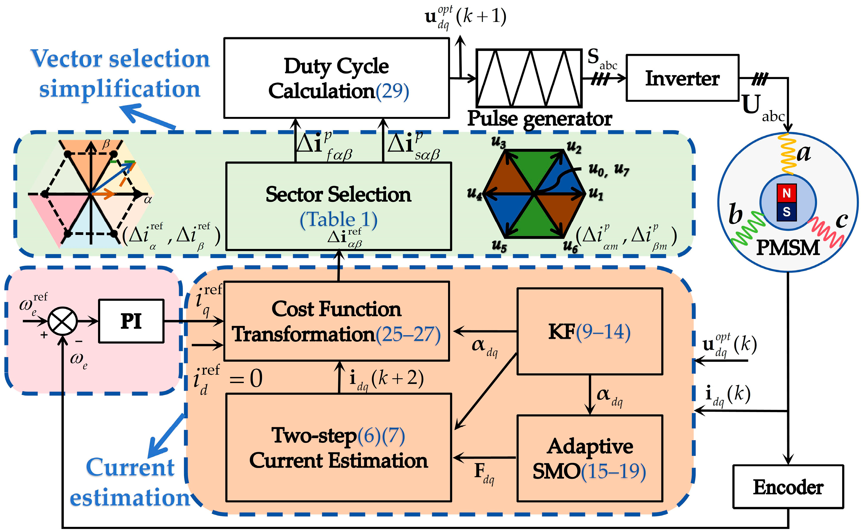
In this article, in order to enhance the accuracy of current estimation in model-free predictive control and streamline the voltage vector selection process. a current ULM based on a KF and an adaptive SMO is proposed. Moreover, by transforming the cost function, a vector selection method based on sector distribution is introduced. The main contributions of this study include:

• A ULM for PMSM current control is developed to reduce dependence on precise motor parameters, thereby enabling highly adaptive control.
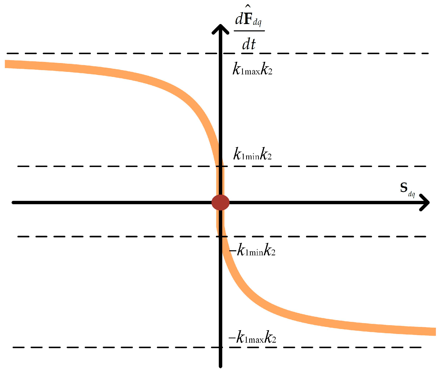
• By designing a KF to monitor current gain and utilizing an adaptive SMO to detect current disturbances, the robustness of the system is enhanced and precise current prediction is realized.
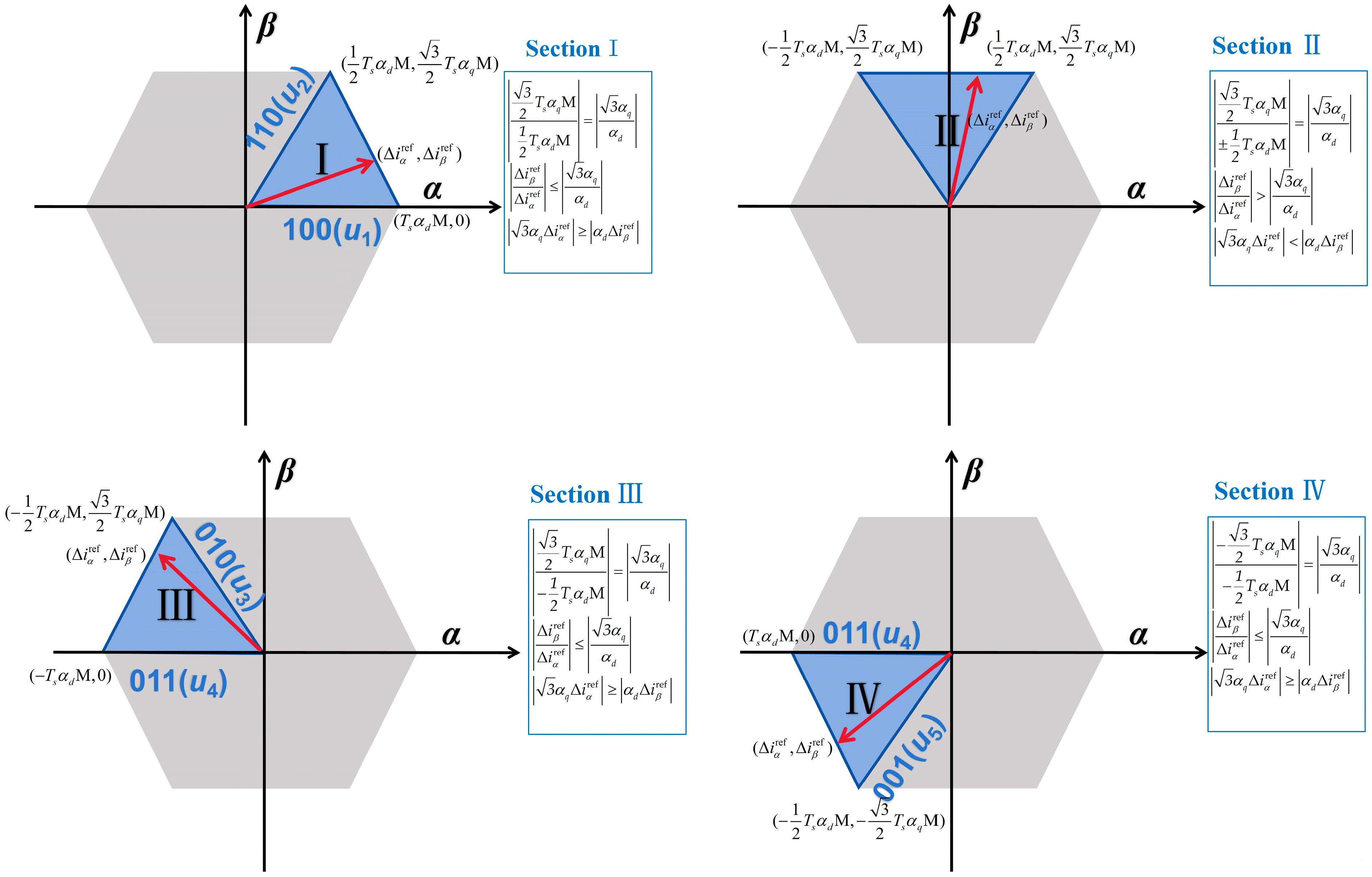
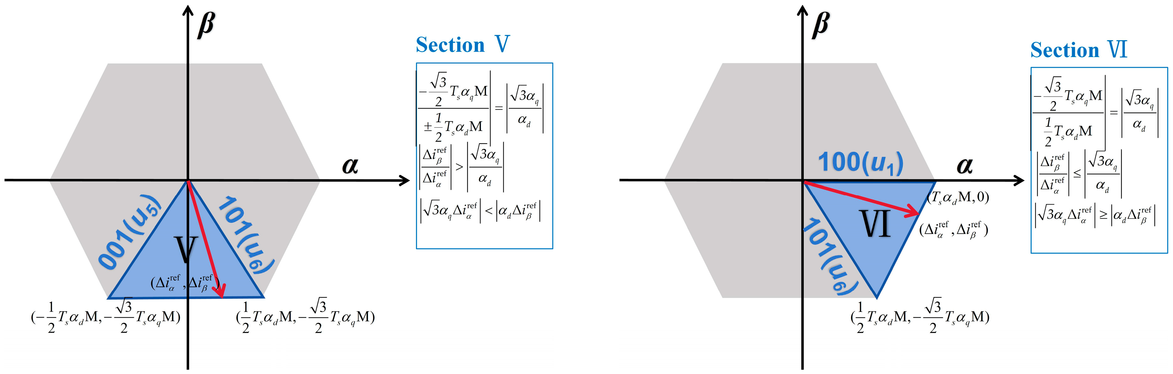
• Based on the developed ULM, an equivalent transformation of the cost function in the αβ reference domain is executed, and a vector selection method based on sector distribution is introduced. The proposed method reduces the six possible voltage vector combinations to a single, unified voltage vector combination, thereby significantly reducing the computational complexity.

This paper is organized as follows. Section 2 presents the mathematical model of the PMSM, followed by the introduction of the MFPCC control strategy, with detailed descriptions of its current estimation and voltage vector simplification processes. In Section 3 and Section 4, simulations and experiments are performed to validate the effectiveness of the proposed control strategy. Finally, a conclusion of this study is given in Section 5.

2. Mathematical Model and Theoretical Foundations

2.1. Mathematical Model of PMSM

The mathematical equation describing a three-phase PMSM in the dq-axis coordinate system can be expressed as:

$${\displaystyle \frac{d{i}_{dq}}{dt}}=A{u}_{dq}+B{i}_{dq}+C$$

(1)

where $i_{dq}=\left[\begin{array}{c}{i}_d\\ i_q\end{array}\right]$, $u_{dq}=\left[\begin{array}{c}{u}_d\\ u_q\end{array}\right]$, $A=\left[\begin{array}{cc}{\displaystyle \frac{1}{L_d}}& 0\\ 0& {\displaystyle \frac{-1}{L_q}}\end{array}\right]$, $B=\left[\begin{array}{cc}{\displaystyle \frac{-R_{\mathrm{s}}}{L_d}}& {\displaystyle \frac{L_q{\omega }_e}{L_d}}\\ {\displaystyle \frac{L_d{\omega }_e}{L_q}}& {\displaystyle \frac{-R_s}{L_q}}\end{array}\right]$, $C=\left[\begin{array}{c}0\\ {\displaystyle \frac{{\omega }_e{\psi }_f}{L_q}}\end{array}\right]$. i_d and i_q represent the current along the dq-axis, respectively; u_d and u_q denote the dq-axis voltages; R_s indicates the stator resistance; ω_e signifies the electric angular speed; and ψ_f represents the stator flux linkage.

By applying the Euler discretization method, Equation (1) can be approximated as:

$$i_{dq}(k+1)=i_{dq}(k)+T_s(A{u}_{dq}(k)+B{i}_{dq}(k)+C)$$

(2)

where $i_{dq}(k+1)=\left[\begin{array}{c}{i}_d(k+1)\\ i_q(k+1)\end{array}\right]$, $i_{dq}(k)=\left[\begin{array}{c}{i}_d(k)\\ i_q(k)\end{array}\right]$, $i_{dq}(k+1)=\left[\begin{array}{c}{i}_d(k+1)\\ i_q(k+1)\end{array}\right]$, $u_{dq}(k)=\left[\begin{array}{c}{u}_d(k)\\ u_q(k)\end{array}\right]$ and T_s represents the sampling time.

The PMSM is driven by a PWM inverter operating in eight distinct switching states. Based on these states, the three-phase voltage equations are derived as:

$$\left\{\begin{array}{c}{U}_{\mathrm{a}}={\displaystyle \frac{U_{\mathrm{dc}}(2S_{\mathrm{a}}-S_{\mathrm{b}}-S_{\mathrm{c}})}{3}}\\ U_{\mathrm{b}}={\displaystyle \frac{U_{\mathrm{dc}}(2S_{\mathrm{b}}-S_{\mathrm{a}}-S_{\mathrm{c}})}{3}}\\ U_{\mathrm{c}}={\displaystyle \frac{U_{\mathrm{dc}}(2S_{\mathrm{c}}-S_{\mathrm{a}}-S_{\mathrm{b}})}{3}}\end{array}\right.$$

(3)

where U_a, U_b, and U_c denote the three-phase voltages; U_dc represents the DC voltage; S_a, S_b, and S_c indicate the inverter switching states. Through various switching configurations, the inverter ultimately produces eight distinct voltage combinations—comprising two zero-voltage states and six active voltage states.

2.2. Proposed MFPCC Algorithm

The complete workflow is illustrated in Figure 1. First, an ultra-local model is adopted to supplant the conventional predictive model reliant on motor parameters (6)(7). The current gain is measured using a Kalman filter (9–14), and the current disturbance is estimated using an adaptive sliding mode observer (15–19). Then, the reference current undergoes a series of transformations in the αβ coordinate domain (25–27), and candidate voltage vectors are selected via sector decomposition (

Table 1. Candidate sector correspondence.

Conditions	Sectors	uf	us	Conditions	Sectors	uf	us
$i_{\alpha }^{\mathrm{ref}}$ ≥ 0	Ⅰ	u1	u2	$i_{\beta }^{\mathrm{ref}}$ ≥ 0 |$\sqrt{3}$αqΔ$i_{\alpha }^{\mathrm{ref}}$| < |αdΔ$i_{\beta }^{\mathrm{ref}}$|	Ⅱ	u2	u3
$i_{\beta }^{\mathrm{ref}}$ ≥ 0
|$\sqrt{3}$αqΔ$i_{\alpha }^{\mathrm{ref}}$| ≥ |αdΔ$i_{\beta }^{\mathrm{ref}}$|
$i_{\alpha }^{\mathrm{ref}}$ ≤ 0	Ⅲ	u3	u4	$i_{\alpha }^{\mathrm{ref}}$ ≤ 0	Ⅳ	u4	u5
$i_{\beta }^{\mathrm{ref}}$ ≥ 0				$i_{\beta }^{\mathrm{ref}}$ ≤ 0
|$\sqrt{3}$αqΔ$i_{\alpha }^{\mathrm{ref}}$| ≥ |αdΔ$i_{\beta }^{\mathrm{ref}}$|				|$\sqrt{3}$αqΔ$i_{\alpha }^{\mathrm{ref}}$| ≥ |αdΔ$i_{\beta }^{\mathrm{ref}}$|
$i_{\beta }^{\mathrm{ref}}$ ≥ 0 |$\sqrt{3}$αqΔ$i_{\alpha }^{\mathrm{ref}}$| < |αdΔ$i_{\beta }^{\mathrm{ref}}$|	Ⅴ	u5	u6	$i_{\alpha }^{\mathrm{ref}}$ ≥ 0	Ⅵ	u6	u1
				$i_{\beta }^{\mathrm{ref}}$ ≤ 0
				|$\sqrt{3}$αqΔ$i_{\alpha }^{\mathrm{ref}}$| ≥ |αdΔ$i_{\beta }^{\mathrm{ref}}$|

). Finally, the dwell time of each candidate vector is calculated to produce the PWM output (29).

2.2.1. ULM Design

Equation (1) indicates that the current equations in the dq-axis coordinate system are highly sensitive to motor parameters; therefore, precise estimation of these parameters is critical for effective MPCC implementation. To enhance prediction robustness, a ULM is employed in place of Equation (1), with its detailed formulation presented below:

$${\displaystyle \frac{d{i}_{dq}}{dt}}={\alpha }_{dq}{u}_{dq}+F_{dq}$$

(4)

where ${\alpha }_{dq}=\left[\begin{array}{cc}{\alpha }_d& 0\\ 0& {\alpha }_q\end{array}\right]$, $F_{dq}=\left[\begin{array}{c}{F}_d\\ F_q\end{array}\right]$; α_d and α_q denote the voltage gains in the dq domain; F_d and F_q represent the unknown disturbances in the dq domain. By applying a discretization scheme, Equation (4) can be approximated as:

$$i_{dq}(k+1)=i_{dq}(k)+T_s({\alpha }_{dq}{u}_{dq}(k)+F_{dq})$$

(5)

To compensate for the inherent control step delay of the motor, a two-step prediction scheme is employed for current forecasting as:

$$i_{dq}^p(k+1)=i_{dq}(k)+T_s({\alpha }_{dq}{u}_{dq}^{opt}(k)+F_{dq})$$

(6)

$$i_{dq}^p(k+2)=i_{dq}^p(k+1)+T_s({\alpha }_{dq}{u}_{dqc}(k)+F_{dq})$$

(7)

where the superscript p denotes the predicted current; ${\mathbf{u}}_{dq}^{opt}$(k) represents the candidate voltage vector computed at time k − 1; u_dqc(k) denotes the candidate voltage vector at the current time; F_dq is assumed to remain constant during the two-step prediction.

The cost function (8) is evaluated by combining multiple candidate voltage vectors.

$$g={[i_d^{\mathrm{ref}}-i_d^p(k+2)]}^2+{[i_q^{\mathrm{ref}}-i_q^p(k+2)]}^2$$

(8)

where $i_d^{\mathrm{ref}}$ and $i_q^{\mathrm{ref}}$ denote the reference currents along the dq axis, respectively, with $i_d^{\mathrm{ref}}$ set to 0 and $i_q^{\mathrm{ref}}$ determined by the outer speed loop. Among the various voltage vector combinations, the one corresponding to the minimum value of the cost function is ultimately selected.

2.2.2. KF-Based Estimation of α_dq

Equation (1) indicates that α_dq equals ${\mathbf{L}}_{dq}^{-}$, where $L_{dq}=\left[\begin{array}{cc}{L}_d& 0\\ 0& L_q\end{array}\right]$. Therefore, if the inductance is known and constant, α_dq would be invariant. In practice, however, precise inductance measurement is challenging, and the inductance may vary with operating conditions. To address this issue, a KF is employed for online estimation of α_dq owing to its rapid convergence, high robustness, and superior noise immunity. The online estimation process of KF is illustrated in Figure 2.

Initially, the parameter α_dq is modeled as a state variable assumed constant or slowly varying over time. From the discrete time model, the state update equation can be expressed as:

$${\widehat{\alpha }}_{dq}^{-}(k)=F{\widehat{\alpha }}_{dq}(k-1)+w_{dq}$$

(9)

where ${\widehat{\alpha }}_{dq}^{-}$ represents the priori state estimate; ${\widehat{\alpha }}_{dq}$ denotes the posteriori state estimate. F is the state matrix, for current gain, $F=\left[\begin{array}{cc}1& 0\\ 0& 1\end{array}\right]$; w_dq represents the process noise accounting for minor variations in the parameter, with its covariance denoted by Q.

In conjunction with Equation (6), the measurement Z_dq is defined as the difference between the present and the previous current values, augmented by the disturbance term. Accordingly, the measurement equation can be expressed as:

$$Z_{dq}(k)=H_{dq}(k){\alpha }_{dq}(k)+V_{dq}$$

(10)

where $Z_{dq}(k)=i_{dq}(k)-i_{dq}(k-1)-T_s\cdot F_{dq}$,$H_{dq}(k)=\left[\begin{array}{cc}{T}_s{u}_d^{opt}(k)& 0\\ 0& T_s{u}_q^{opt}(k)\end{array}\right]$; V_dq denotes the measurement noise, with its covariance given by R.

The predicted covariance matrix is given by:

$$P_{dq}^{-}(k)=F{P}_{dq}(k-1)F^T+Q$$

(11)

where ${\mathbf{P}}_{dq}^{-}$ denotes the covariance between the true and predicted values; P_dq denotes the covariance between the true values and the optimal estimated values. Subsequently, following the KF principles, the Kalman gain K_g is computed to achieve optimal correction of the state estimate:

$$K_g(k)={\displaystyle \frac{P_{dq}^{-}(k)H_{dq}^T(k)}{H_{dq}(k)P_{dq}^{-}(k)H_{dq}^T(k)+R}}$$

(12)

Subsequently, the state variables are corrected and updated to achieve a more precise state estimation:

$${\widehat{\alpha }}_{dq}(k)={\widehat{\alpha }}_{dq}^{-}(k)+K_g(k)(Z_{dq}(k)-H_{dq}(k){\widehat{\alpha }}_{dq}^{-}(k))$$

(13)

Finally, the covariance matrix is updated to accurately capture the most recent changes in state estimation uncertainty, thereby ensuring the posteriori estimate attains optimal statistical performance:

$$P_{dq}(k)=\left[\begin{array}{c}I-K_g(k)H_{dq}(k)\end{array}\right]P_{dq}^{-}(k)$$

(14)

In the system, the inductance variation amplitude is small. Therefore, the process noise covariance is set as $Q=\left[\begin{array}{cc}0.01& 0\\ 0& 0.01\end{array}\right]$, and the measurement noise covariance is set as $R=\left[\begin{array}{cc}0.01& 0\\ 0& 0.01\end{array}\right]$, ensuring that the estimate of ${\widehat{\alpha }}_{dq}$ remains smooth.

2.2.3. Adaptive SMO-Based Estimation of F_dq

In order to estimate F_dq, an adaptive SMO is designed as Figure 3.

Initially, from (4), the SMO can be conducted as:

$$\left\{\begin{array}{c}{\displaystyle \frac{d{\widehat{i}}_{dq}}{dt}}={\alpha }_{dq}{u}_{dq}+{\widehat{F}}_{dq}+M_{smo}\\ {\displaystyle \frac{d{\widehat{F}}_{dq}}{dt}}=k_1{M}_{smo}\end{array}\right.$$

(15)

where ${\widehat{i}}_{dq}=\left[\begin{array}{c}{\widehat{i}}_d\\ {\widehat{i}}_q\end{array}\right]$, ${\widehat{F}}_{dq}=\left[\begin{array}{c}{\widehat{F}}_d\\ {\widehat{F}}_q\end{array}\right]$, $M_{smo}=\left[\begin{array}{c}{M}_{dsmo}\\ M_{qsmo}\end{array}\right]$. ${\widehat{i}}_d$ and ${\widehat{i}}_q$ are the predicted dq-axis current, respectively; ${\widehat{F}}_d$ and ${\widehat{F}}_q$ are the corresponding components of the unknown disturbance estimate in the dq-axis. The scalar k₁ denotes the sliding mode observer gain, and M_dsmo and M_qsmo are the sliding mode control functions for the dq-axis.

Selecting ${\widehat{i}}_{dq}$ as the observed output, the sliding surface is defined as:

$$S_{dq}={\widehat{i}}_{dq}-i_{dq}$$

(16)

where $S_{dq}=\left[\begin{array}{c}{S}_d\\ S_q\end{array}\right]$. The sliding mode control function employed is given by:

$$M_{smo}=-k_2\mathrm{sign}(S_{dq})$$

(17)

where k₂ denotes the sliding mode control parameter (k₂ >  0); sign() is a symbolic function which can be expressed as:

$$\mathrm{sign}(x)=\left\{\begin{array}{c}-1,\hspace{1em}x<0\hfill \\ 0,\hspace{1em} x=0\hfill \\ 1,\hspace{1em} x>0\hfill \end{array}\right.$$

(18)

To prevent high-frequency chattering as the system approaches the sliding surface, the sliding mode observer gain is adaptively adjusted according to:

$$k_1=k_{1\min }+(k_{1\max }-k_{1\min }){\displaystyle \frac{\left|S_d\right|+\left|S_q\right|}{\left|S_d\right|+\left|S_q\right|+G}}$$

(19)

where k_1min and k_1max represent the lower and upper bounds of the sliding mode control parameters; G > 0 is a smoothing parameter. Consequently, the rate of change of the current disturbance is depicted in Figure 4.

By combining Equations (4), (15) and (16), the derivative of S_dq is obtained as:

$${\displaystyle \frac{d{S}_{dq}}{dt}}=E_{F_{dq}}+M_{smo}$$

(20)

where $E_{F_{dq}}=\left[\begin{array}{c}{E}_{F_d}\\ E_{F_q}\end{array}\right]={\widehat{F}}_{dq}-F_{dq}$.

Theorem 1.

The SMO method demonstrates stability and ultimately converges during the iterative process.

Proof of Theorem 1.

The stability of the system is established through a Lyapunov function:

$$V_f=0.5S_{dq}^T{S}_{dq}=0.5(S_d^2+S_q^2)$$

(21)

According to Lyapunov theory, system stability requires that the derivative of V_f be negative:

$${\displaystyle \frac{d{V}_f}{dt}}=S_d{\displaystyle \frac{d{S}_d}{dt}}+S_q{\displaystyle \frac{d{S}_q}{dt}}<0$$

(22)

By combining Equations (17) and (20), Equation (22) can be simplified as follows:

$${\displaystyle \frac{d{V}_f}{dt}}=S_d(E_{F_d}-k_2\mathrm{sign}(S_d))+S_q(E_{F_q}-k_2\mathrm{sign}(S_q))<0$$

(23)

The resulting constraint on k₂ can thus be written as:

$$k_2>\max (|E_{F_d}|,|E_{F_q}|)$$

(24)

If k₂ satisfies Equation (24), it can be proven that SMO ultimately converges during the iterative process. □

2.3. Simplification of the Candidate Vector

A vector selection method based on sector distribution mitigates the combinatorial explosion of voltage vector combinations and the attendant computational burden in conventional model predictive control by reducing six candidate vector combinations to a single representative vector. First, Equation (8) is reformulated as:

$$g={[\mathsf{\Delta }{i}_d^{\mathrm{ref}}-\mathsf{\Delta }{i}_d^p(k+2)]}^2+{[\mathsf{\Delta }{i}_q^{\mathrm{ref}}-\mathsf{\Delta }{i}_q^p(k+2)]}^2$$

(25)

where

$$\left\{\begin{array}{c}\mathsf{\Delta }{i}_d^{\mathrm{ref}}=i_d^{\mathrm{ref}}-i_d^p(k+1)-T_s{F}_d\\ \mathsf{\Delta }{i}_d^p(k+2)=i_d^p(k+2)-i_d^p(k+1)-T_s{F}_d=T_s{\alpha }_d{u}_{dc}(k)\\ \mathsf{\Delta }{i}_q^{\mathrm{ref}}=i_q^{\mathrm{ref}}-i_q^p(k+1)-T_s{F}_q\\ \mathsf{\Delta }{i}_q^p(k+2)=\mathsf{\Delta }{i}_q^p(k+2)-i_q^p(k+1)-T_s{F}_q=T_s{\alpha }_q{u}_{qc}(k)\end{array}\right.$$

For the cost function g, it is interpreted as the distance between Δ${\mathbf{i}}_{dq}^{\mathrm{ref}}$ and Δ${\mathbf{i}}_{dq}^p$(k + 2) in the dq domain, which is equivalent to the distance between Δ${\mathbf{i}}_{\alpha \beta }^{\mathrm{ref}}$ and Δ${\mathbf{i}}_{\alpha \beta }^p$(k + 2) in the αβ domain. The transformation equation between the dq and αβ coordinate systems can be presented as:

$$\left[\begin{array}{cc}\mathsf{\Delta }{i}_{\alpha }^{\mathrm{ref}}\hfill & \mathsf{\Delta }{i}_{\alpha }^p(k+2)\\ \mathsf{\Delta }{i}_{\beta }^{\mathrm{ref}}\hfill & \mathsf{\Delta }{i}_{\beta }^p(k+2)\end{array}\right]=\left[\begin{array}{cc}cos({\theta }_e)& -sin({\theta }_e)\\ sin({\theta }_e)& cos({\theta }_e)\end{array}\right]\left[\begin{array}{cc}\mathsf{\Delta }{i}_d^{\mathrm{ref}}\hfill & \mathsf{\Delta }{i}_d^p(k+2)\\ \mathsf{\Delta }{i}_q^{\mathrm{ref}}\hfill & \mathsf{\Delta }{i}_q^p(k+2)\end{array}\right]$$

(26)

where θ_e is the electrical angle. Therefore, Equation (25) can be further reformulated as:

$$g_l={[\mathsf{\Delta }{i}_{\alpha }^{\mathrm{ref}}-\mathsf{\Delta }{i}_{\alpha }^p(k+2)]}^2+{[\mathsf{\Delta }{i}_{\beta }^{\mathrm{ref}}-\mathsf{\Delta }{i}_{\beta }^p(k+2)]}^2$$

(27)

where $\mathsf{\Delta }{i}_{\alpha }^p(k+2)=T_s{\alpha }_d{u}_{\alpha c}(k)$, $\mathsf{\Delta }{i}_{\beta }^p(k+2)=T_s{\alpha }_q{u}_{\beta c}(k)$; u_αc and u_βc denote the candidate voltage vectors in the αβ domain.

In the αβ domain, the distribution of Δ${\mathbf{i}}_{\alpha \beta }^p$ under varying L_d and L_q conditions is illustrated in Figure 5. The blue vectors represent Δ$i_{sm}^p$ (m∈{0, 1, …,6}), which are independently generated from six distinct effective voltage vectors in addition to the zero-voltage vector.

As shown in Figure 6, once the magnitudes of Δ$i_{\alpha }^{\mathrm{ref}}$, Δ$i_{\beta }^{\mathrm{ref}}$ are determined, it is only necessary to identify the position of (Δ$i_{\alpha }^{\mathrm{ref}}$, Δ$i_{\beta }^{\mathrm{ref}}$) within the αβ coordinate system. Based on Table 1 (detailed explanations can be found in Appendix A), the corresponding sector can be selected, which then facilitates the identification of the candidate voltage vector combination.

Once the candidate vector combinations have been determined, Δ$i_{\alpha }^{\mathrm{ref}}$ and Δ$i_{\beta }^{\mathrm{ref}}$ can be expressed in terms of candidate combinations as:

$$\left\{\begin{array}{c}\mathsf{\Delta }{i}_{\alpha }^{\mathrm{ref}}=d_f\cdot \mathsf{\Delta }{i}_{\alpha f}^p(k+2)+d_s\cdot \mathsf{\Delta }{i}_{\alpha \mathrm{s}}^p(k+2)\\ \mathsf{\Delta }{i}_{\beta }^{\mathrm{ref}}=d_f\cdot \mathsf{\Delta }{i}_{\beta f}^p(k+2)+d_s\cdot \mathsf{\Delta }{i}_{\beta s}^p(k+2)\end{array}\right.$$

(28)

where the subscripts f and s represent the first and second candidate vectors; symbol d denotes the duty cycle of the applied vector.

By Equation (28), the values of d_f and d_s can be derived as:

$$\left\{\begin{array}{c}{d}_f={\displaystyle \frac{\mathsf{\Delta }{i}_{\alpha \mathrm{s}}^p(k+2)\cdot \mathsf{\Delta }{i}_{\beta }^{\mathrm{ref}}-\mathsf{\Delta }{i}_{\beta f}^p(k+2)\cdot \mathsf{\Delta }{i}_{\alpha }^{\mathrm{ref}}}{\mathsf{\Delta }{i}_{\alpha \mathrm{s}}^p(k+2)\mathsf{\Delta }{i}_{\beta f}^p(k+2)-\mathsf{\Delta }{i}_{\alpha f}^p(k+2)\mathsf{\Delta }{i}_{\beta f}^p(k+2)}}\\ d_s={\displaystyle \frac{\mathsf{\Delta }{i}_{\beta f}^p\cdot (k+2)\mathsf{\Delta }{i}_{\alpha }^{\mathrm{ref}}-\mathsf{\Delta }{i}_{\alpha f}^p(k+2)\cdot \mathsf{\Delta }{i}_{\beta }^{\mathrm{ref}}}{\mathsf{\Delta }{i}_{\alpha \mathrm{s}}^p(k+2)\mathsf{\Delta }{i}_{\beta f}^p(k+2)-\mathsf{\Delta }{i}_{\alpha f}^p(k+2)\mathsf{\Delta }{i}_{\beta f}^p(k+2)}}\end{array}\right.$$

(29)

Due to the discrepancy between the predicted and actual currents, d_f + d_s may exceed 1, potentially affecting the subsequent current prediction process. Therefore, the values of d_f and d_s must be adjusted as specified in

Table 2. Duty cycle boundary constraints.

Conditions	df	ds
df + ds > 1, df ≤ 1	df	1 − df
df + ds > 1, df > 1	1	0
else	df	ds

to ensure they remain within a reasonable range. When d_f + d_s > 1, priority should be given to maintaining the value of d_f, while restricting d_s. If d_f > 1, set d_f = 1 and d_s = 0.

3. Simulation Results and Analysis

To validate the effectiveness of the proposed MFPCC method, simulations and experiments were conducted on a 2 kW PMSM, with comparison against the MPCC FCS-MFPCC [20] and PFPCC [30] methods. The parameters of the PMSM are provided in

Table 3. Main parameters of PMSM.

Symbol	Quantity	Value
p	Number of pole pairs	4
Rs	Stator resistance	0.4 Ω
Ld	Direct axis inductance	9 mH
Lq	Quadrature axis inductance	9 mH
ψf	Permanent magnet flux	0.1667 Wb
Udc	DC-bus voltage	220 V

. All simulations and experiments were conducted with a control and sampling frequency of 10 kHz with optimal parameters. The detailed simulation parameters are shown in

Table 4. Main parameters of Simulation.

Simulation Configuration	Parameters
Software	MATLAB/SIMULINK
Type	Fixed-step
Solver	ode3 (Bogacki-Shampine)
Sampling frequency	10 kHz
Control frequency	10 kHz
Default torque	2 N·S
Default reference speed	1000 r/min

. The PI controller parameters for the speed loop were set to K_p = 0.1 and K_i = 3; the SMO parameters were k_1min = 500, k_1max = 100, k₂ = 2000, and G = 0.5; the KF parameters were ${\alpha }_d^{\mathrm{initial}}$ = 160, ${\alpha }_q^{\mathrm{initial}}$ = 160, $Q=\left[\begin{array}{cc}0.01& 0\\ 0& 0.01\end{array}\right]$ and $R=\left[\begin{array}{cc}0.01& 0\\ 0& 0.01\end{array}\right]$, where ${\alpha }_d^{\mathrm{initial}}$ and ${\alpha }_q^{\mathrm{initial}}$ represent the initial value of the dq-axis current gain. More detailed model parameter settings are provided in the Appendix A (

Table A1. Combinations of different voltage vectors.

Combination	(${\mathit{u}}_{\mathit{\alpha }}$, ${\mathit{u}}_{\mathit{\beta }}$)	Combination	(${\mathit{u}}_{\mathit{\alpha }}$, ${\mathit{u}}_{\mathit{\beta }}$)
100	(M, 0)	110	$(1/2\mathrm{M},\sqrt{3}$/2M)
010	$(-1/2\mathrm{M},\sqrt{3}$/2M)	011	(-M, 0)
001	$(-1/2\mathrm{M},-\sqrt{3}$/2M)	101	$(1/2\mathrm{M},-\sqrt{3}$/2M)
000	(0, 0)	111	(0, 0)

).

3.1. Comparison of Simulation Efficiency

To evaluate the effectiveness of the vector simplification algorithm, a comprehensive evaluation of its computational performance and real-time capability was conducted using the Simulink environment in conjunction with the Profiler tool under a load torque of 2 N·m and a reference speed of 1000 r/min. Figure 7 illustrates the single-call execution times for four approaches: MPCC, FCS-MFPCC, PFPCC, and the proposed MFPCC. The results reveal that the proposed MFPCC accelerates computation by 60.8% compared with the conventional MPCC, and by 38.9% and 33.5% relative to FCS-MFPCC and PFPCC. These quantitative findings demonstrate that the proposed vector simplification strategy significantly enhances real-time execution efficiency, highlighting its superior performance in high-frequency application scenarios.

3.2. Stability Analysis of ULM Under Simulation Condition

To evaluate the stability of the proposed ULM, tests were conducted under a load torque of 2 N·m and a reference speed of 1000 r/min. Figure 8 illustrates the variations in the current gains α_dq and disturbances F_dq. Simulation results indicate that during the startup phase, α_d stabilizes at 403 ms and α_q at 212 ms, with their final steady-state values approaching ${\mathbf{L}}_{dq}^{-}$. Meanwhile, F_d exhibits a positive peak and F_q shows a negative impulse. Subsequently, the disturbances along both dq axes rapidly converge and remain within minimal fluctuation ranges after 98 ms and 114 ms, respectively. These results demonstrate that the proposed ULM exhibits excellent performance in steady-state regulation.

3.3. Dynamic Response Analysis of KF and SMO

According to Equation (1), the values of current gain are inversely proportional to the inductance. To evaluate the dynamic response capability of KF, simulations were conducted under two scenarios: L_dq increased to 150% and decreased to 50% of its original value under a load torque of 2 N·m and a reference speed of 1000 r/min. As illustrated in Figure 9a, when L_dq is increased to 150% of its original value, α_d stabilizes at 423 ms and α_q at 214 ms—both values corresponding to a reduction of ${\mathbf{L}}_{dq}^{-}$ to 66.7%. Figure 9b shows that when L_dq is decreased to 50% of its original value, α_d and α_q stabilize at 397 ms and 241 ms, respectively, which is equivalent to an effective scaling of 200%. These findings indicate that when the motor parameters vary dynamically, the model can promptly respond and converge to the true parameter values, due to the adaptive correction of KF based on the discrepancy between the actual and predicted currents, thereby ensuring efficient convergence of the parameter estimation.

The current disturbance F_dq is closely associated with the motor speed and torque. To evaluate the dynamic response capability of the designed SMO, simulations were conducted under two scenarios: a step increase in torque from 2 N·m to 5 N·m at 0.4 s, while maintaining a constant speed of 1000 r/min, and a step increase in speed from 1000 r/min to 1500 r/min at 0.4 s, while maintaining a constant torque of 2 N·m. As illustrated in Figure 10, under the torque step condition, F_d stabilizes rapidly within 11.6 ms, while F_q stabilizes rapidly within 4.5 ms. Conversely, Figure 11 demonstrates that under the speed step condition, F_d stabilizes within 18.5 ms, while F_q reaches stability within 12.5 ms. Therefore, the SMO enables rapid disturbance estimation under system variations, effectively maintaining system stability.

3.4. Analysis of Current Fluctuations Under Simulation Condition

Figure 12 presents the simulation curves of I_d, I_q, and the three-phase current I_abc for MPCC, FCS-MFPCC, and the proposed MFPCC under conditions of ideal motor parameters and stable operating conditions. The results indicate that the proposed MFPCC provides I_q tracking performance comparable to that of conventional MPCC and FCS-MFPCC, while exhibiting notable improvements in the stability of I_d tracking and lower noise levels, thereby enhancing precision and overall system robustness. To clearly present the performance metrics,

Table 5. E_sd, E_sq,THD under ideal motor parameters.

Method	Esd (A)	Esq (A)	THD
MPCC	0.0738	0.0462	3.20%
FCS-MFPCC	0.1930	0.0432	6.94%
Proposed MFPCC	0.0189	0.0375	1.64%

summarizes the standard deviation of the dq-axis current (E_sd,E_sq), and the total harmonic distortion (THD) of the three-phase currents. The data results indicate that the THD achieved by the proposed MFPCC is significantly lower than that for both MPCC and FCS-MFPCC.

3.5. Robustness Test

To evaluate the robustness of the proposed MFPCC, simulations were conducted with the motor parameters adjusted to 150% R_L, 80% L_d, 80% L_q, and 80% ψ_f. Figure 13 presents the simulation results for MPCC, FCS-MFPCC, and the proposed MFPCC. When the actual motor parameters deviate from their nominal values, MPCC control causes I_d to deviate slightly from zero and I_q to diverge markedly from its reference. This discrepancy arises from strong dependence on the motor parameters, leading to substantial mismatches between the estimated and actual values. In contrast, both FCS-MFPCC and the proposed MFPCC effectively suppress deviations in the I_dq, although the FCS-MFPCC still exhibits notable current fluctuations. Furthermore, owing to its more accurate current prediction, the proposed MFPCC exhibits a markedly lower THD than the other two methods (

Table 6. E_sd, E_sq, THD under 150% R_L, 80% L_dq, and 80% ψ_f.

Method	Esd (A)	Esq (A)	THD
MPCC	0.0554	0.0261	2.76%
FCS-MFPCC	0.1267	0.0495	3.90%
Proposed MFPCC	0.0123	0.0166	0.65%

).

4. Experiment Results and Analysis

The experimental setup used a 2 kW permanent magnet synchronous motor, with parameters consistent with the simulation values presented in Table 3. Photographs of the assembled hardware platform are shown in Figure 14. In this configuration, the controlled motor is mechanically linked to a load motor via a coupling, with a torque-speed sensor installed at the interface to enable real-time monitoring of both torque and speed. These measurements are transmitted to the host computer via a communication cable. The load motor is connected to a general purpose inverter that controls the application and removal of load. Additionally, the experimental motor is equipped with a 2500-line incremental rotary encoder, with its rotational direction, position, and speed measured and computed using the enhanced quadrature encoder pulse (eQEP) module embedded in the controller’s primary chip, the TMS320F28377D. This dual-core chip from Texas Instruments concurrently executes the control algorithms and processes the communication signals. Additionally, peripheral devices—such as the analog-to-digital conversion (ADC) module, enhanced pulse-width modulation (ePWM) module, and serial communication interface (SCI) module—are used for voltage and current A/D data sampling, motor control algorithm calculations, power transistor switching signal output, and transmitting experimental data to the host computer for monitoring. The drive circuitry features an Infineon intelligent IPM module that responds to fault signals (including overvoltage, overcurrent, and overtemperature conditions) by interrupting the power transistor drive signals, thereby protecting the system.

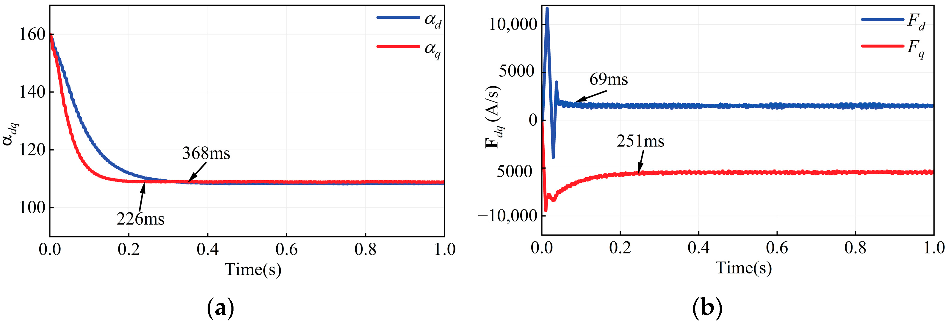
4.1. Stability Analysis of ULM Under Experimental Condition

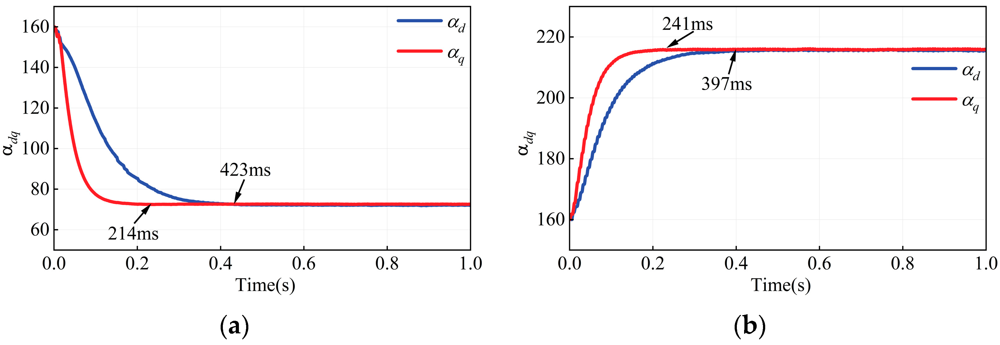
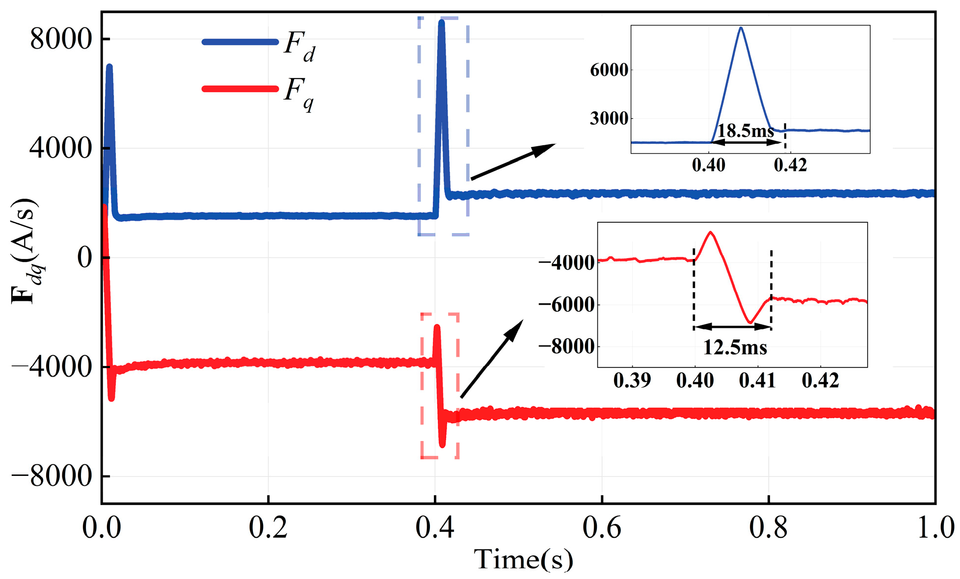
To validate the stability of the proposed ULM, experiments were conducted under a load torque of 2 N·m and a reference speed of 1000 r/min. Figure 15 illustrates the evolution of α_dq and F_dq during the transition from startup to steady-state operation. The results indicate that α_d and α_q stabilize at 368 ms and 226 ms, respectively, with their steady-state values closely approximating ${\mathbf{L}}_{dq}^{-}$. Similarly, F_d and F_q stabilize at 69 ms and 251 ms. These findings clearly demonstrate the superior performance of the proposed ULM.

4.2. Vector Distribution Analysis

To visually demonstrate the proposed vector selection method, Figure 16a,b depict the steady-state fluctuation characteristics of Δ$i_{\alpha }^{\mathrm{ref}}$ and Δ$i_{\beta }^{\mathrm{ref}}$, respectively, under steady-state conditions and scatter distribution in the αβ coordinate system with a load torque of 2 N·m and a reference speed of 1000 r/min. As illustrated in Figure 16a, during system stability, $i_{\alpha }^{\mathrm{ref}}$ and Δ$i_{\beta }^{\mathrm{ref}}$ exhibit periodic sinusoidal waveforms with a distinct phase difference between them. Meanwhile, Figure 16b shows that the distribution of these two variables in the αβ coordinate domain is relatively compact, forming an overall circular trajectory. Based on the sector position of each data point, appropriate candidate vectors are subsequently selected.

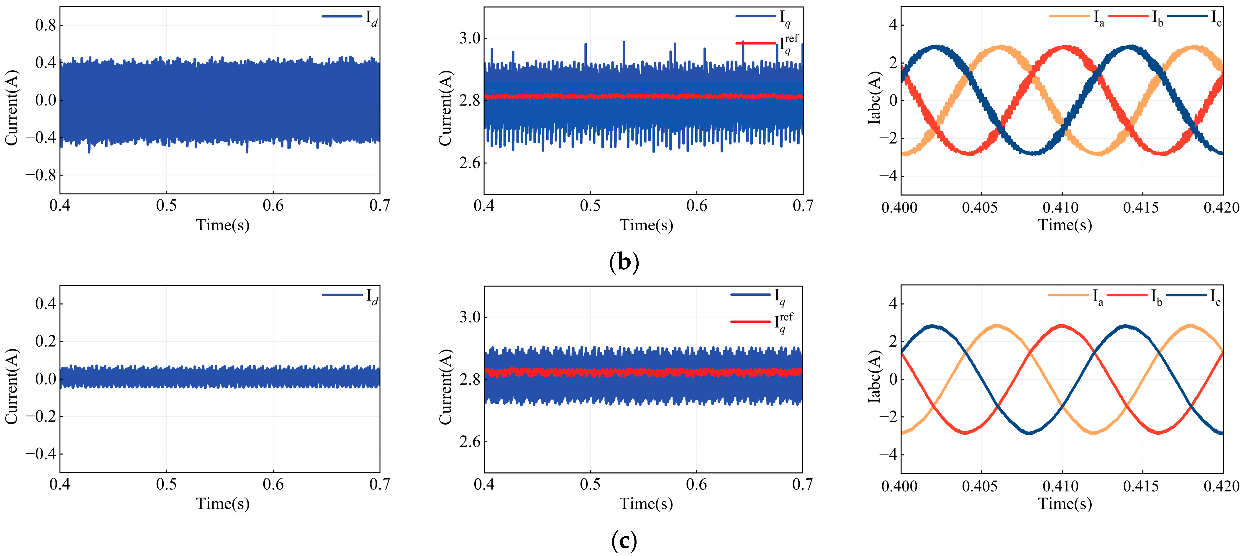
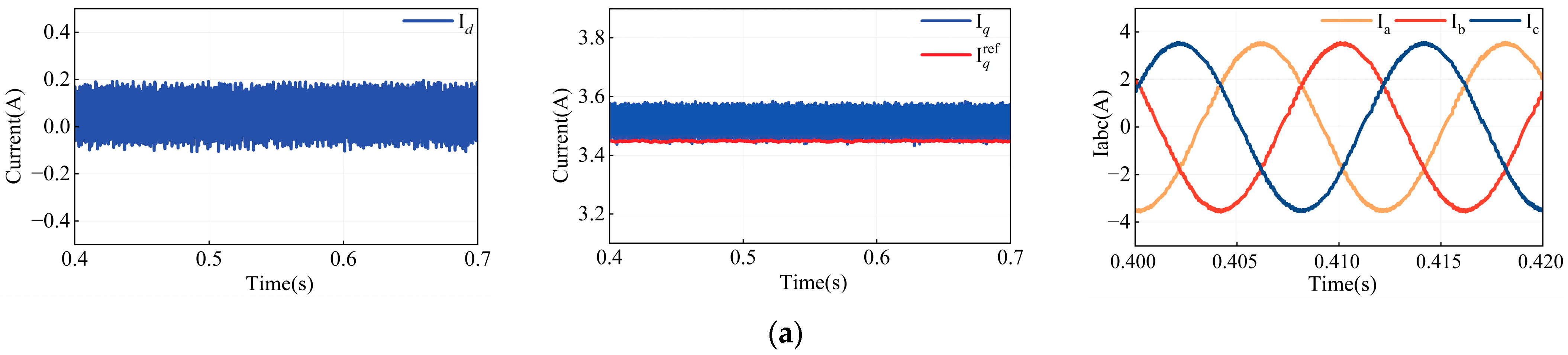
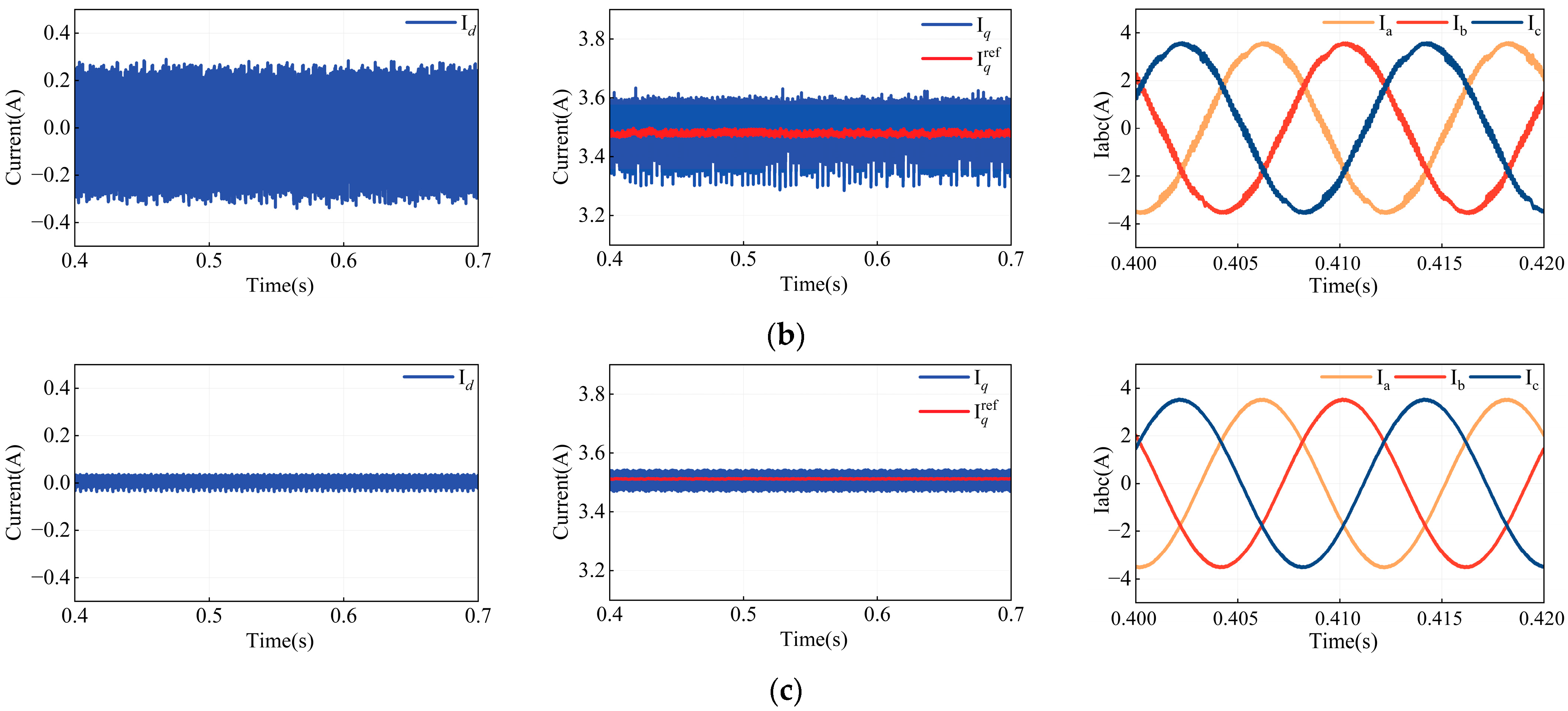
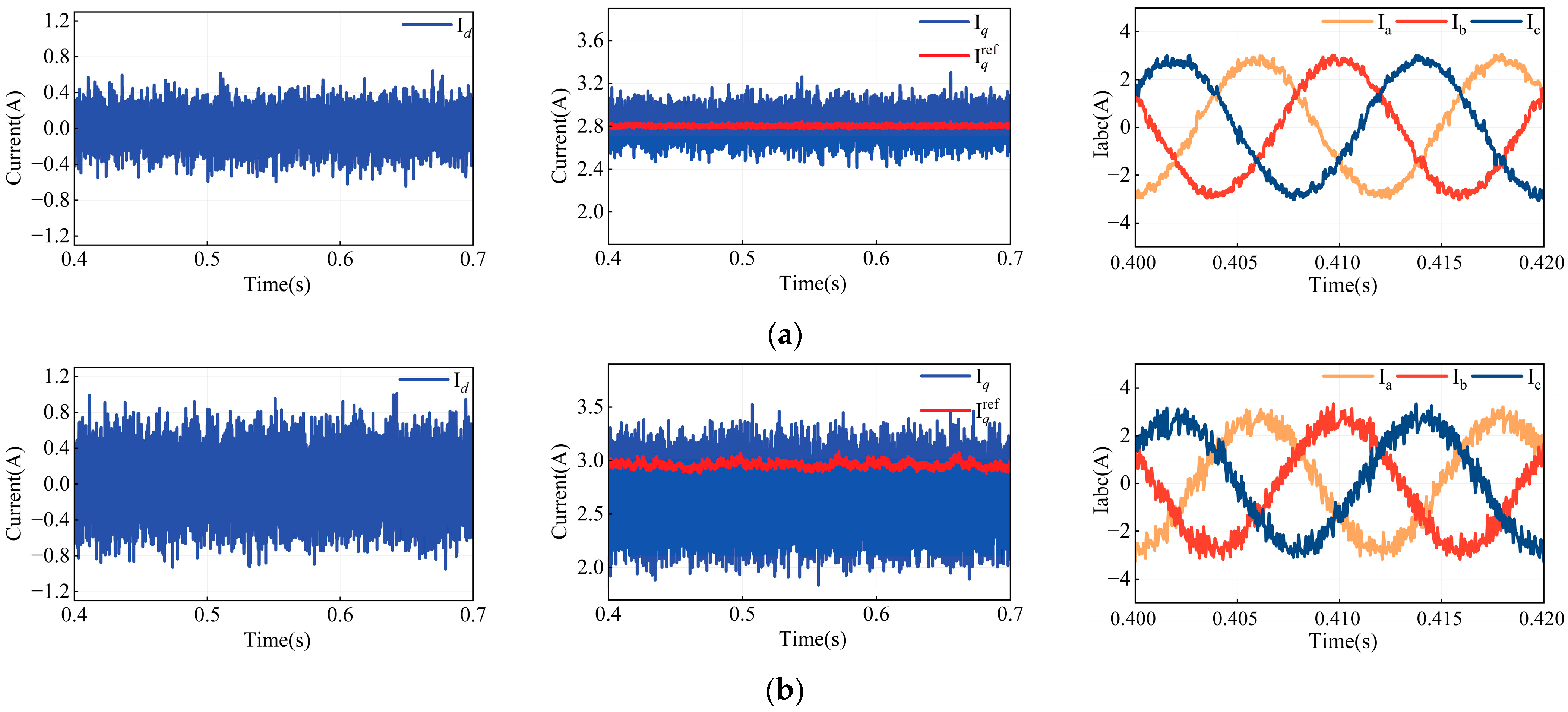
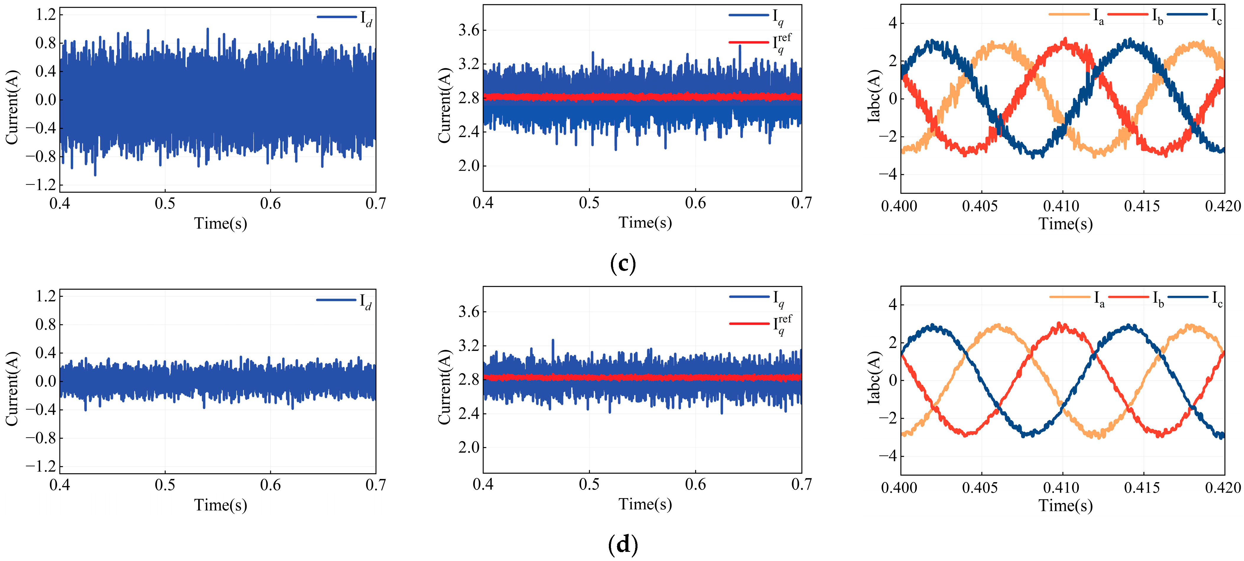
4.3. Analysis of Current Fluctuations Under Experimental Condition

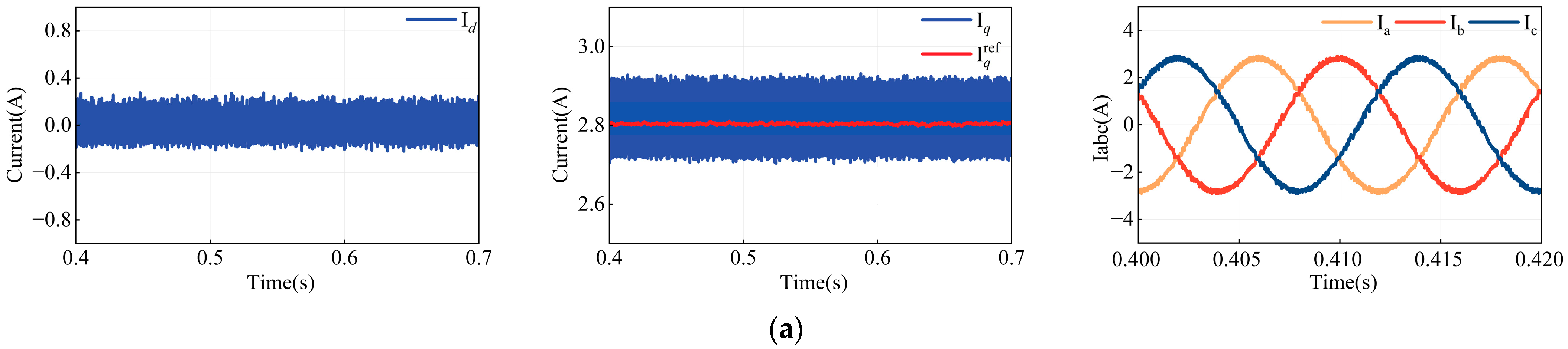
Figure 17 presents the steady-state current fluctuations for MPCC (with accurately known motor parameters), MPCC (with model parameter L_dq set to 50% of its original value), FCS-MFPCC, and the proposed MFPCC under a load torque of 2 N·m and a reference speed of 1000 r/min.

Table 7. E_sd, E_sd, THD under different control methods.

Method	Esd (A)	Esq (A)	THD
MPCC (100% L)	0.1615	0.1087	6.68%
MPCC (50% L)	0.2710	0.2436	12.77%
FCS-MFPCC	0.2717	0.1370	10.37%
Proposed MFPCC	0.0977	0.1031	5.08%

summarizes the corresponding values of E_sd, E_sq, and THD. The results indicate that with accurate MPCC parameter settings, the I_dq are minimal, with E_sd = 0.1615 A, E_sq = 0.1087 A, and a low THD of 6.68%. However, when the model parameters are inaccurate, E_sd and E_sq increase by 67.8% and 132.4%, respectively, and THD rises by 6.09%, along with a significant deviation of the I_q from its reference.

Since both FCS-MFPCC and the proposed MFPCC are parameter-independent, they effectively prevent current deviation from the reference value. Nevertheless, the FCS-MFPCC method exhibits notable I_d fluctuations, with E_sd = 0.2717 A, E_sq = 0.1370 A, and THD at 10.37%. In contrast, the proposed MFPCC demonstrates superior performance, achieving E_sd = 0.0977 A, E_sq = 0.1031 A, and a THD of only 5.08%. These results confirm that the proposed MFPCC accurately predicts system behavior without relying on model parameters, thereby ensuring robust system stability.

4.4. Robustness Assessment

Multiple experimental series were conducted under conditions of inductance parameter mismatch to further evaluate the robustness of the model under a load torque of 2 N·m and a reference speed of 1000 r/min. The integral of time and absolute error (ITAE) (30) [31] are measured as shown in Figure 18 to evaluate the response time and current tracking performance in the dq-axis.

$$\mathrm{ITAE}={\displaystyle \int t\left|e(t)\right|dt}$$

(30)

where e(t) denotes the d-axis (q-axis) current tracking error. Experiments were conducted under a load torque of 2 N·m and a reference speed of 1000 r/min within 2s. Under inductance parameter mismatch, MPCC exhibits significant degradation in both current response and tracking performance along the dq-axis. FCS-MFPCC, by contrast, shows pronounced sensitivity in the d-axis current response and tracking, while the q-axis current remains largely unaffected. The proposed MFPCC is inherently robust to such parameter mismatches, as it leverages KF to perform online estimation of the inductance and operates independently of fixed model parameters. This characteristic highlights the superior robustness of the proposed MFPCC in terms of current response and tracking under inductance uncertainty.

5. Conclusions

This paper presents an MFPCC method for PMSMs. The proposed approach constructs a current prediction model based on a ULM, which utilizes a KF and an adaptive SMO to estimate the current gain and disturbances. A vector selection method based on sector distribution is then employed to choose candidate voltage vectors, thereby eliminating reliance on motor parameters inherent in traditional approaches and significantly improving computational efficiency. Simulation and experiment were successfully conducted on a 2 kW PMSM and the following conclusions were drawn:

• In comparison with MPCC, FCS-MFPCC, and PFPCC, the proposed MFPCC method exhibits a notable enhancement in computational efficiency.
• The proposed MFPCC approach ensures that both the current gain and current disturbance converge to stable states rapidly.
• The proposed MFPCC demonstrates a rapid dynamic response to fluctuations in the system parameters, such as load torque variations or sudden changes in rotational speed.
• When the system parameters are accurately modeled, the proposed MFPCC exhibits superior performance in mitigating current harmonics compared to the conventional MPCC and FCS-MFPCC. Conversely, under parameter mismatch scenarios, the proposed MFPCC demonstrates robust current tracking capabilities.

However, the performance of the proposed method under severe system fluctuations has not been fully addressed, and further research will be conducted in this direction in the future.

References

1. Dai, Y.; Song, L.; Cui, S. Development of PMSM drives for hybrid electric car applications. IEEE Trans. Magn. 2007, 43, 434–437. [Google Scholar] [CrossRef]
2. Yuan, T.; Wang, D.; Wang, X.; Wang, X.; Sun, Z. High-precision servo control of industry robot driven by PMSM-DTC utilizing composite active vectors. IEEE Access 2019, 7, 7577–7587. [Google Scholar] [CrossRef]
3. Li, P.; Xu, X.; Yang, S.; Jiang, X. Open circuit fault diagnosis strategy of PMSM drive system based on grey prediction theory for industrial robot. Energy Rep. 2023, 9, 313–320. [Google Scholar] [CrossRef]
4. Perez Mayo, A.; Saenz-Aguirre, A.; Martin, F.; Vadillo, J. FOC-droop control strategy for PMSM fed paralleled multi-inverter power systems oriented to aeronautical applications. Electr. Power Syst. Res. 2020, 185, 106369. [Google Scholar] [CrossRef]
5. Mesloub, H.; Boumaaraf, R.; Benchouia, M.T.; Golea, A.; Golea, N.; Srairi, K. Comparative study of conventional DTC and DTC_SVM based control of PMSM motor—Simulation and experimental results. Math. Comput. Simul. 2020, 167, 296–307. [Google Scholar] [CrossRef]
6. Wang, X.; Shen, J.; Sun, S.; Xiao, D.; Liu, Y.; Wang, Z. General modeling and control of multiple three-phase PMSM drives. IEEE Trans. Power Electron. 2025, 40, 1900–1909. [Google Scholar] [CrossRef]
7. Koiwa, K.; Kuribayashi, T.; Zanma, T.; Liu, K.-Z.; Wakaiki, M. Optimal current control for PMSM considering inverter output voltage limit: Model predictive control and pulse-width modulation. IET Electr. Power Appl. 2019, 13, 2044–2051. [Google Scholar] [CrossRef]
8. Kawai, H.; Cordier, J.; Kennel, R.; Doki, S. Application of finite control set-model predictive control for servo brake motion in PMSM drives. IEEE Can. J. Electr. Comput. Eng. 2023, 46, 117–129. [Google Scholar] [CrossRef]
9. Benakcha, M.; Benakcha, A.; Abdessemed, R.; Zouzou, S.E. Sensorless real-time implementation-based FS-MPCC and deadbeat predictive control with delay and dead-time compensation of PMSM using MRAS and T-S fuzzy speed controller. Electr. Eng. 2023, 105, 4139. [Google Scholar] [CrossRef]
10. Hossen, M.B.; Habibullah, M. Robust Model-Free Predictive Torque Control for Induction Motor Drive Based on an Ultralocal Model. IEEE Access 2025, 13, 47514–47524. [Google Scholar] [CrossRef]
11. Zhu, Z.; Wei, X.; Han, R.; Liu, C.; Zhang, Z. Double-Vector Model-Free Predictive Current Control for PMSMs With Influence Rejection of DC Voltage Mismatch. IEEE Trans. Transp. Electrif. 2025, 11, 6143–6153. [Google Scholar] [CrossRef]
12. Wang, S.; Fan, H.; Zhao, J. Model-Free Predictive Current Control of DTP-PMSM Based on Ultra-Local Model Considering Back EMF Harmonics. IEEE J. Emerg. Sel. Top. Power Electron. 2025, 13, 553–563. [Google Scholar] [CrossRef]
13. Liu, Z.; Huang, X.; Hu, Q.; Yang, G.; Wang, Y.; Shen, J. Model-Free Predictive Current Control of PMSM Using Modified Extended State Observer. IEEE Trans. Power Electron. 2025, 40, 679–690. [Google Scholar] [CrossRef]
14. Wang, Y.; Liao, W.; Huang, S.; Zhang, J.; Yang, M.; Li, C.; Huang, S. A Robust DPCC for IPMSM Based on a Full Parameter Identification Method. IEEE Trans. Ind. Electron. 2023, 70, 7695–7705. [Google Scholar] [CrossRef]
15. Zhang, X.; Cao, Y. A Simple Motor-Parameter-Free Model Predictive Current Control for PMSM Drive. IEEE Trans. Ind. Electron. 2025, 72, 3292–3302. [Google Scholar] [CrossRef]
16. Zhang, X.; Zhang, C.; Wang, Z.; Rodriguez, J. Motor-parameter-free model predictive current control for PMSM drives. IEEE Trans. Ind. Electron. 2024, 71, 5443–5452. [Google Scholar] [CrossRef]
17. Feng, Y.; Zhang, S.; Zhang, C. An improved model-free predictive current control for PMSM under low-speed condition. IEEE J. Emerg. Sel. Top. Power Electron. 2024, 12, 555–565. [Google Scholar] [CrossRef]
18. Zhang, Y.; Jin, J.; Huang, L. Model-free predictive current control of PMSM drives based on extended state observer using ultralocal model. IEEE Trans. Ind. Electron. 2021, 68, 993–1003. [Google Scholar] [CrossRef]
19. Lin, C.-K.; Liu, T.-H.; Yu, J.-T.; Fu, L.-C.; Hsiao, C.-F. Model-free predictive current control for interior permanent-magnet synchronous motor drives based on current difference detection technique. IEEE Trans. Ind. Electron. 2014, 61, 667–681. [Google Scholar] [CrossRef]
20. Sun, Z.; Deng, Y.; Wang, J.; Yang, T.; Wei, Z.; Cao, H. Finite control set model-free predictive current control of PMSM with two voltage vectors based on ultralocal model. IEEE Trans. Power Electron. 2023, 38, 776–788. [Google Scholar] [CrossRef]
21. Lammouchi, Z.; Naoui, M.; Bekakra, Y.; Khechekhouche, A.; Sbita, L. Model-Free Predictive Control Based on the Execution Time of Active Vectors Using Ultra-Local Model. Arab. J. Sci. Eng. 2025, 50, 5885–5898. [Google Scholar] [CrossRef]
22. Li, H.; Lan, D.; Shao, J.; Tahir, M. Model-Free Predictive Current Control of PMSM with Online Current Gradient Updating Using Ultra-Local Model. IEEE Trans. Energy Convers. 2025. [Google Scholar] [CrossRef]
23. Zhou, Y.; Zhang, S.; Zhang, C.; Li, X.; Li, X.; Yuan, X. Current Prediction Error Based Parameter Identification Method for SPMSM With Deadbeat Predictive Current Control. IEEE Trans. Energy Convers. 2021, 36, 1700–1710. [Google Scholar] [CrossRef]
24. Dang, D.Q.; Rafaq, M.S.; Choi, H.H.; Jung, J.W. Online Parameter Estimation Technique for Adaptive Control Applications of Interior PM Synchronous Motor Drives. IEEE Trans. Ind. Electron. 2016, 63, 1438–1449. [Google Scholar] [CrossRef]
25. Jabbour, N.; Mademlis, C. Online Parameters Estimation and Autotuning of a Discrete-Time Model Predictive Speed Controller for Induction Motor Drives. IEEE Trans. Power Electron. 2019, 34, 1548–1559. [Google Scholar] [CrossRef]
26. Zhang, X.; Hou, B.; Mei, Y. Deadbeat Predictive Current Control of Permanent-Magnet Synchronous Motors with Stator Current and Disturbance Observer. IEEE Trans. Power Electron. 2017, 32, 3818–3834. [Google Scholar] [CrossRef]
27. Su, J.; Sun, D. Simplified MPCC for four-switch three-phase inverter-fed PMSM. Electron. Lett. 2017, 53, 1108–1109. [Google Scholar] [CrossRef]
28. Wen, D.; Li, Z.; Wei, X.; Cheng, Z. Simplified three-vector selection model predictive current control for PMSM considering fixed switching frequency. Prog. Electromagn. Res. C 2024, 143, 199–207. [Google Scholar] [CrossRef]
29. Zhang, Y.; Xu, D.; Liu, J.; Gao, S.; Xu, W. Performance improvement of model-predictive current control of permanent magnet synchronous motor drives. IEEE Trans. Ind. Appl. 2017, 53, 3683–3695. [Google Scholar] [CrossRef]
30. Zhu, Z.; Wei, X.; Yu, F.; Zhang, Z. Overmodulatable parameter-free predictive current control for PMSMs. IEEE Trans. Power Electron. 2025, 40, 1774–1786. [Google Scholar] [CrossRef]
31. Bartoszewicz, A.; Nowacka-Leverton, A. ITAE Optimal Sliding Modes for Third-Order Systems with Input Signal and State Constraints. IEEE Trans. Autom. Control 2010, 55, 1928–1932. [Google Scholar] [CrossRef]
Figure 1. Schematic of the proposed MFPCC architecture.
Energies 18 03049 g001
Figure 2. Schematic of the KF estimation process.
Energies 18 03049 g002
Figure 3. Block diagram of the adaptive SMO.
Energies 18 03049 g003
Figure 4. Variation curve of sliding mode control function.
Energies 18 03049 g004
Figure 5. Distribution of Δ i s m p under different inductance conditions.
Energies 18 03049 g005
Figure 6. Block diagram of current vector synthesis.
Energies 18 03049 g006
Figure 7. Comparison of per-invocation execution times across different methods.
Energies 18 03049 g007
Figure 8. Simulation results of proposed MFPCC under a torque of 2 N·m and a reference speed of 1000 r/min. (a) Current gain coefficient αdq; (b) Current disturbance Fdq.
Energies 18 03049 g008
Figure 9. Simulation results of αdq for the proposed MFPCC under different operating conditions. (a) Ldq increased to 150% of its original values; (b) Ldq decreased to 50% of its original values.
Energies 18 03049 g009
Figure 10. Simulation results of Fdq for the proposed MFPCC under a step increase in torque from 2 N·m to 5 N·m at 0.4 s.
Energies 18 03049 g010
Figure 11. Simulation results of Fdq for the proposed MFPCC under a step increase in speed from 1000 r/min to 1500 r/min at 0.4 s.
Energies 18 03049 g011
Figure 12. Simulation results for the dq-axis and three-phase currents at a torque of 2 N·m and a reference speed of 1000 r/min under ideal motor parameters. (a) MPCC; (b) FCS-MFPCC; (c) Proposed MFPCC.
Energies 18 03049 g012aEnergies 18 03049 g012b
Figure 13. Simulation results for the dq-axis and three-phase currents at a torque of 2 N·m and a reference speed of 1000 r/min under 150% RL, 80% L, and 80% ψf. (a) MPCC; (b) FCS-MFPCC; (c) Proposed MFPCC.
Energies 18 03049 g013aEnergies 18 03049 g013b
Figure 14. PMSM experimental platform.
Energies 18 03049 g014
Figure 15. The experimental results of the proposed MFPCC under a torque of 2 N·m and a reference speed of 1000 r/min. (a) Current gain coefficient αdq; (b) current disturbance Fdq.
Energies 18 03049 g015
Figure 16. Vector selection analysis of proposed MFPCC at a torque of 2 N·m and a reference speed of 1000 r/min. (a) The time-varying curve of i α β ref ; (b) the spatial distribution of i α β ref in the αβ coordinate domain.
Energies 18 03049 g016
Figure 17. Experiment results for the dq-axis and three-phase currents at a torque of 2 N·m and a reference speed of 1000 r/min under different control method. (a) MPCC (with model parameters fully matching the motor parameters); (b) MPCC (with Ldq set to 50% of original value while the remaining parameters match the motor); (c) FCS-MFPCC; (d) Proposed MFPCC.
Energies 18 03049 g017aEnergies 18 03049 g017b
Figure 18. Experimental results of dq-axis current ITAE values under inductance mismatch. (a) d-axis; (b) q-axis.
Energies 18 03049 g018