Article

Development of Recurrent Neural Networks for Thermal/Electrical Analysis of Non-Residential Buildings Based on Energy Consumptions Data

by
Elisa Belloni
1,*,
Flavia Forconi
2,
Gabriele Maria Lozito
3,
Martina Palermo
2,
Michele Quercio
2 and
Francesco Riganti Fulginei
2
1
Department of Engineering, University of Perugia, 06125 Perugia, Italy
2
Department of Industrial, Electronic and Mechanical Engineering, Roma Tre University, 00146 Rome, Italy
3
Department of Information Engineering, University of Firenze, 50139 Firenze, Italy
*
Author to whom correspondence should be addressed.
Energies 2025, 18(12), 3031; https://doi.org/10.3390/en18123031
Submission received: 14 April 2025 / Revised: 29 May 2025 / Accepted: 4 June 2025 / Published: 7 June 2025
(This article belongs to the Special Issue Environmental Sustainability and Energy Economy)

Abstract

Extensive research has focused on optimizing energy consumption in residential buildings based on indoor thermal conditions. However, modeling the energy and thermal behavior of non-residential buildings presents greater challenges due to their complex geometries and the high computational cost of detailed simulations. Simplifying input variables can enhance the applicability of artificial intelligence techniques in predicting energy and thermal performance. This study proposes a neural network-based approach to characterize the thermal–energy relationship in commercial buildings, aiming to provide an efficient and scalable solution for performance prediction. Consumptions trends for a building are generated using the EnergyPlus™ dynamic simulation software over a timespan of a year in different locations, and the data are then used to train neural network models. Uncertainty analyses are carried out to evaluate the behavior effectiveness of the artificial neural networks (ANNs) in different weather conditions, and the root mean square error (RMSE) is calculated in terms of mean air temperatures. The results show that this approach can reproduce the functional relationship between input and output data. Three different ANNs are trained for the northern, central, and southern climatic zones of Italy. The southern region’s models achieved the highest accuracy, with an RMSE below 0.5 °C; whereas the model for the northern cities was less accurate, since no specific trend in plant management was present, but it still achieved an acceptable accuracy of 1.0 °C. This approach is computationally lightweight; inference time is below 5 ms, and can be easily embedded in optimization algorithms for load dispatch or in microcontroller applications for building automation systems.

1. Introduction

Buildings represent a significant opportunity for cost-effective demand-side management, as they are the primary consumers of electricity in both Europe and the United States. In the U.S., approximately 75% of total electricity consumption is attributed to buildings. In this context, the U.S. Department of Energy (DOE), through the Building Technologies Office (BTO), published a technical report on the opportunities for grid-interactive efficient buildings [1]. The scenario in the USA shows that today primary energy use in buildings is about 41% (22% for residential and 19% for commercial type). In Europe, primary energy for buildings reaches 65% of the total amount, split into 43% for households and 22% for commercial buildings. At the EU level, two-thirds of the building’s consumption is therefore residential [2,3]. Nevertheless, for the residential sector in Europe only 33% of the buildings consumption is covered by electricity, natural gas is still the most widely used energy source by households (35%). Different scenarios are observed for commercial and non-residential buildings. The increasing energy demand in the commercial sector is due to the many air-conditioned commercial buildings, mostly in metropolitan areas [4,5,6,7].
Many studies have been related to the importance of forecasting the energy consumption for these kinds of buildings. The relevant studies have shown the possibility of determining the thermal and electrical loads of commercial [8,9,10,11,12,13,14,15,16,17,18,19,20,21,22,23,24] or residential buildings [25,26,27] through algorithmic approaches, such as artificial neural networks (ANNs). Robinson et al. [8] presented a novel technique for the estimation of commercial buildings loads: several models were used for the training (energy consumption of different case studies in New York city) and were then applied in Atlanta cases to obtain an aggregate energy consumption dataset. The models could be also applied in other U.S. areas exploiting this method. In [10], the authors developed a short-term electrical load estimation algorithm that considers the variation in building operation. In this case non-residential buildings were chosen and, specifically, five commercial buildings of five different types. The case studies were also positioned in different countries all over the world. The most important focus is short-term load forecasting procedures (STLF) (from 1 h to 1 week). The deep learning algorithms proposed in this work allow for the load forecasting framework that is more accurate than similar models in the literature (with an improvement of 20–45%). In [13], a predictive control strategy in a commercial building energy management system (BEMS) was proposed for the management of boilers, where the neural network also takes into account the environmental conditions and the maintenance of the control levels. The BEMS uses real-time automatic control techniques, and it make buildings more intelligent.
Due to the interaction between occupants and buildings, occupancy behavior is irregular and difficult to model, which indirectly introduces uncertainties in the energy use of the building systems and plants [28,29,30,31]. Therefore, by predicting how many people will be in a building in a specific period, systems such as heating, ventilation, and lighting can be regulated more efficiently. An interesting study [30] analyzed the relationship between occupancy, air conditioning usage, and tolerance temperatures in office buildings in China, proposing a control strategy that takes multiple behavioral patterns into account. The consideration of the multiple impacts of the users’ behavior on building energy efficiency allows for accurate energy performance predictions and the adoption of optimization strategies. Forecasting building energy consumption for enhancing flexibility services, controlling building energy systems, and reducing the carbon footprint of the building stock is widely discussed in some other interesting review papers [32,33,34]. A review of the role of artificial intelligence in home energy management systems (HEMS) was presented in [32]. HEMS is fundamental for the optimization of energy consumption and the reduction of electricity costs in smart grids (SGs). For the correct operation of these applications, smart meters are important to track the bidirectional flows of energy, and the integration of renewables (RES), energy storage systems (ESS), electric vehicles (EVs), and other electricity devices are essential.
Another interesting case study is described in [17], the object of which was the energy analysis of commercial buildings. The daily electricity demand was evaluated by means of the EnergyPlus program [35], and an ANN model was developed in MATLAB r2024. This ANN can predict energy consumption for lighting, cooling, and other equipment with mean errors of 13%, 8%, and 4%, respectively. In a paper written by Afzal et al. [14], three different artificial neural networks and regression models were used to predict cooling and heating loads, and the results were compared. A hybrid model was proposed (biogeography-based optimization (BBO) algorithm together with an extreme learning machine (ELM)), and the results demonstrated it was the best one in terms of correlation factor for the estimation of the consumptions. In these wide scenarios, one of the main purposes is the optimization of the building performance that can be obtained by the implementation of techniques that are complex and computationally expensive, above all for the description of the shape and form of the buildings, their thermal behavior, and their insulation features [36,37,38,39]. This is the reason why ANNs are able to replace detailed building models whose simulations are time-consuming. In [37], it was shown that neural networks with multi-objective optimization algorithms represent a good solution to improve energy efficiency and indoor thermal comfort. Also, in [40], a genetic algorithm (GA) with multi-objective functions (cooling energy consumption, discomfort hours, equivalent carbon emissions to be minimized) was proposed, and the authors obtained excellent optimization results with a reduction of electricity consumption of about 40%, with a decrease of discomfort hours equal to 63%. To overcome the problems related to the low accuracy of surrogate models, ANNs are used as an interaction between input and output data for many types of building stock [41,42].
Another important application of ANNs were carried out by Wong et al. [39]. The authors applied ANNs to predict the electricity consumed by office buildings for heating, cooling, and lighting. Also, in this case, simulations were carried out in EnergyPlus [35] to obtain a daily building energy load database for the training and testing of the ANNs. Excellent predictive ANNs were obtained, above all for the forecasting of the electrical demand for lighting. A modeling method for cooling and heating loads prediction was proposed by Chou and Bui [43] with an approach that considered both support vector regression (SVR) and ANNs; an absolute percentage error lower than 4% was obtained with effective and accurate results.
Furthermore, the electricity use in buildings is a key energy factor when also considering the implementation of renewables for the distributed generation of photovoltaic (PV) technologies [44,45,46,47]. The implementation of smart grids and smart buildings to cover this electricity demand in a cost-effective way is fundamental for minimizing greenhouse gas emissions [6]. The integration of intermittent renewable sources implies the dynamic management of smart buildings, and accurate forecasting of electricity consumption is therefore necessary. This is the final aim of a research paper carried out by Belloni et al. [47,48,49,50]: in the first work [47], a computationally lean neural network was developed based on a dataset obtained from a model of the E+ program [35] allowing for the prediction of the thermal–electrical behavior of a building. The added value of these works is the use of these models among a renewable energy community (REC) in which the PV plant generation is also considered for the balance of the loads [50]. In general, machine learning tools are valuable solutions for a variety of applications at the building level or within the context of an energy community (EC), particularly for load forecasting and EC optimization [51,52,53,54].
The work presented in this study investigates using recurrent neural networks (RNNs) as a black-box model for estimating a building’s thermal behavior. The primary objective is to create a model that generalizes well to different climatic conditions and has low computational overhead, enabling its use in building management systems, optimization algorithms for RECs, and embedded applications. In particular, a case study of thermal and energy demand in HVAC systems for a commercial building in different Italian locations, is considered. The selected building is modeled in terms of geometry, insulation features, and HVAC system, and the simulations are carried out in many Italian cities characterized by different weather conditions (global solar radiation, mean air temperatures, relative humidity). Combining the use of a dynamic simulation software with an ANN is another innovative aspect of this approach; the building simulation program can characterize buildings and model their features (envelopes, exposures, geometry, HVAC systems and other electrical devices). Once properly trained with data obtained from the simulations, the ANN will be able to recreate the behavior of buildings in many different locations and environmental conditions. Three different Italian climatic categories are considered, and four cities for each of these categories (for a total number of simulating scenarios equal to twelve). The proposed approach can also be extended to other countries providing the same input data for the ANNs (mean air temperatures, global solar radiation, relative humidity, and wind speed), as well as electrical consumption for heating or cooling purposes. This data can be collected, measured, or derived from meteorological files in other countries.
The remainder of this paper is structured as follows: in Section 2 the methodology and the overall approach to the problem is described. The case study analyzed in this work is described along with the modelling of the office/commercial building in the EnergyPlus program, specifying the assumptions and the boundary conditions. Section 2.3 and Section 2.4 show the general features of the ANN models, with details on the architecture, the input and outputs, and the training hyperparameters. In Section 3.1, the results are analyzed in terms of thermal/electric model output (electricity consumptions for heating/cooling and internal thermal behavior) obtained with the E+ models. Section 3 and Section 4 describe the validation of the ANNs and the critical discussion of the results, respectively. Future works, limitations, and potential are discussed in Section 5. Conclusions and final remarks close the manuscript.

2. Materials and Methods

2.1. Approach

This study aims at developing an RNN model for a commercial/office building located in central Italy by applying a novel method able to correlate the mean inside air temperatures with the hourly energy consumptions of the building itself. The first stage of this approach is the creation of a dataset for the RNN training, for which the methodology is shown in Figure 1.
The EnergyPlus™ (E+) software (version 23.2.0) [35,55] is used to simulate the case study and model the building’s thermal behavior. This program is particularly suited for analyzing heat transmission through opaque and transparent envelopes, making it ideal for complicated geometry and for highly glazed buildings [56]. The program is used to evaluate the electrical energy demand for different profiles of HVAC heating and cooling, for zone programs and loads, for lighting systems, and for people’s occupancy throughout the year. A large dataset is obtained for the training of the RNNs, configured with inputs and outputs with the aim to estimate the internal temperature profile knowing the electrical loads obtained from the E+ simulations.
Twelve datasets of simulation cases are created; each one composed of 8760 vector samples related to hourly energy consumption and mean air temperatures inside the building. Each dataset considers a geographical location for one of twelve Italian cities, grouped by climate
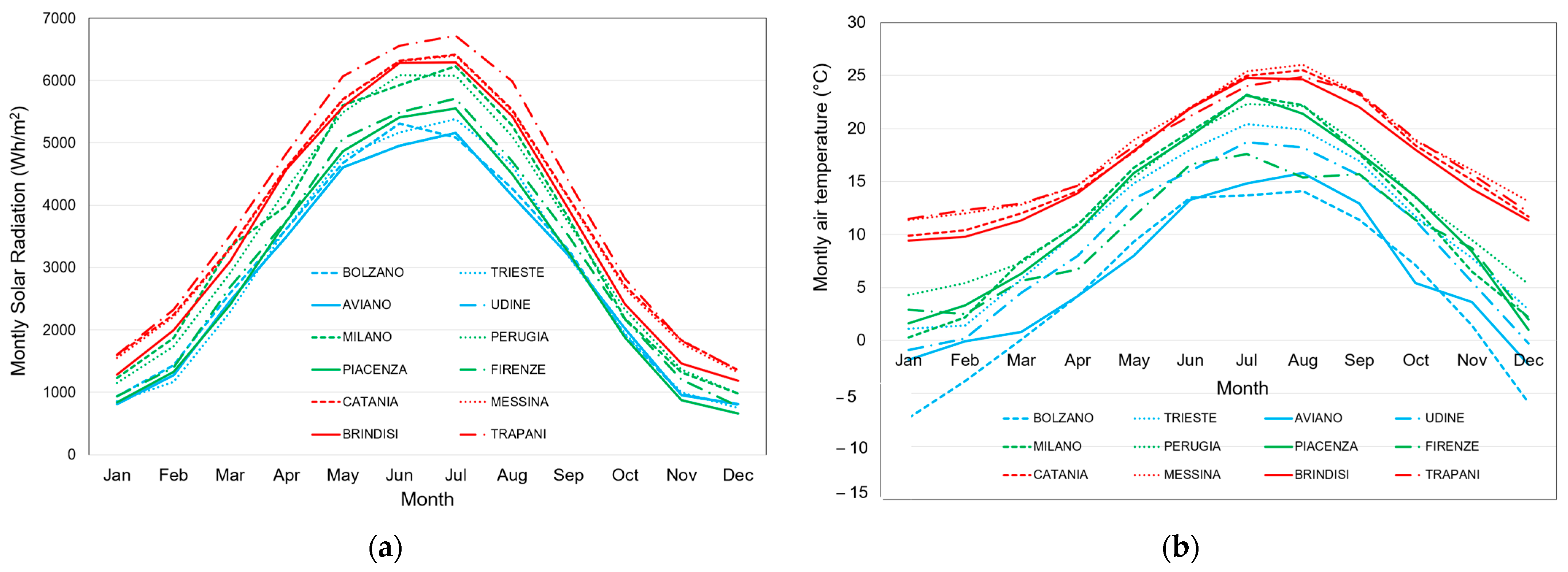
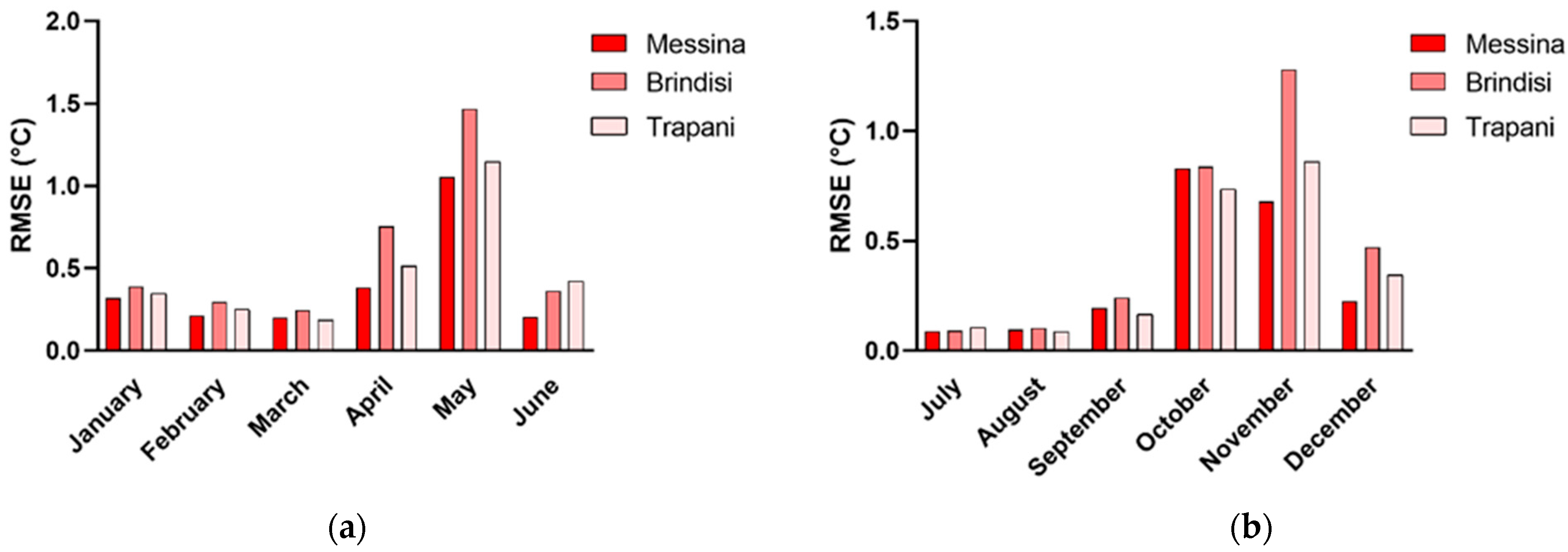
  • Brindisi, Trapani, Messina, and Catania—southern regions with a warm climate.
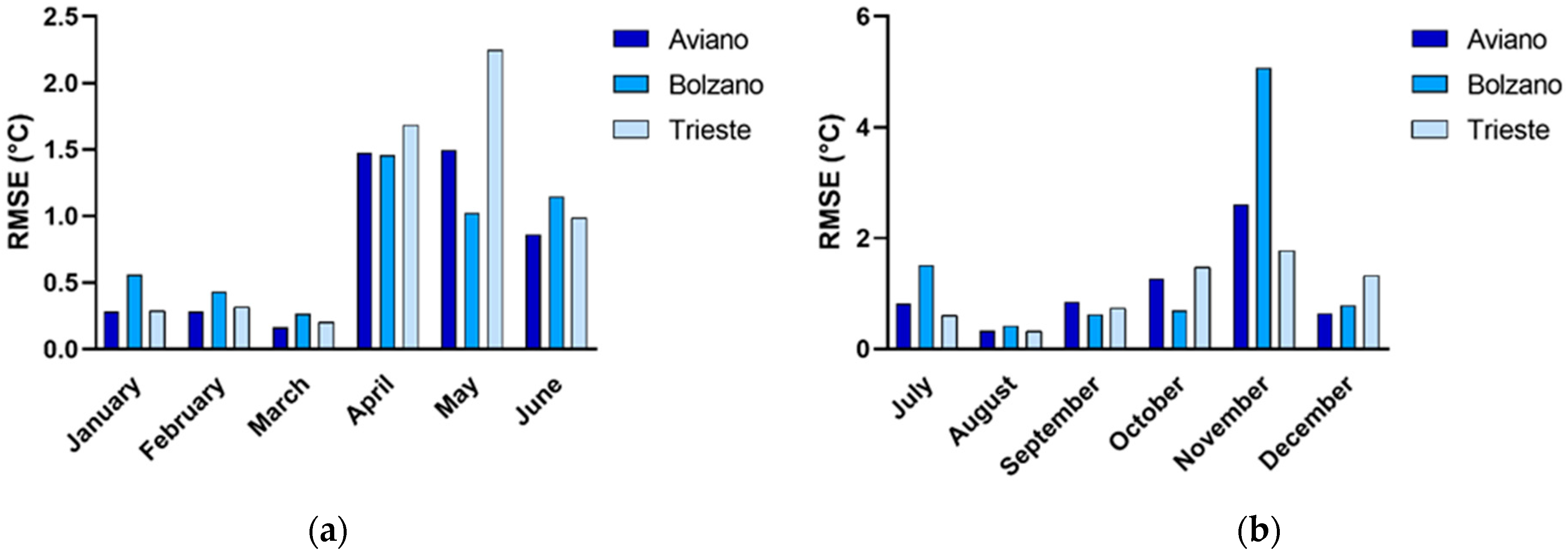
  • Bolzano, Trieste, Aviano, Udine—northern regions with a typical cold mountain climate.
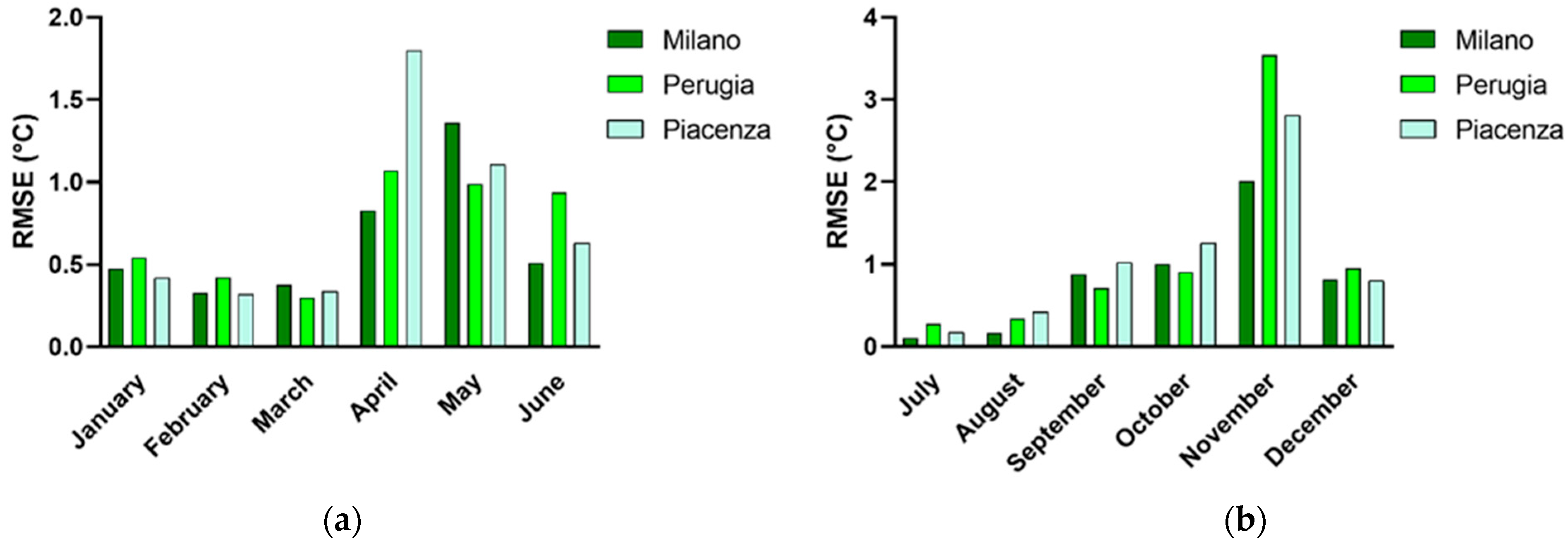
  • Milano, Firenze, Piacenza, and Perugia—central regions with an intermediate climate.
The thermostat of each zone in the E+ setting is programmed to allow for the mean air temperatures to be valued inside a range that maintains comfort conditions both in the winter and in the summer.
The dataset was then used to create a standard training dataset for a neural network, considering a standard 70%/30% division for training, validation, and testing. The datasets were used to train three different RNNs (one for each climate type) and used for the estimation of the thermal behavior of the building when the electricity consumption is given. The neural networks were designed with a gradual increase in weight and connection complexity to preserve their ability to generalize. To prevent overfitting, early stopping techniques were also applied during the training process. Additionally, the training and inference times of the networks were profiled to verify the methodology’s low computational demands.

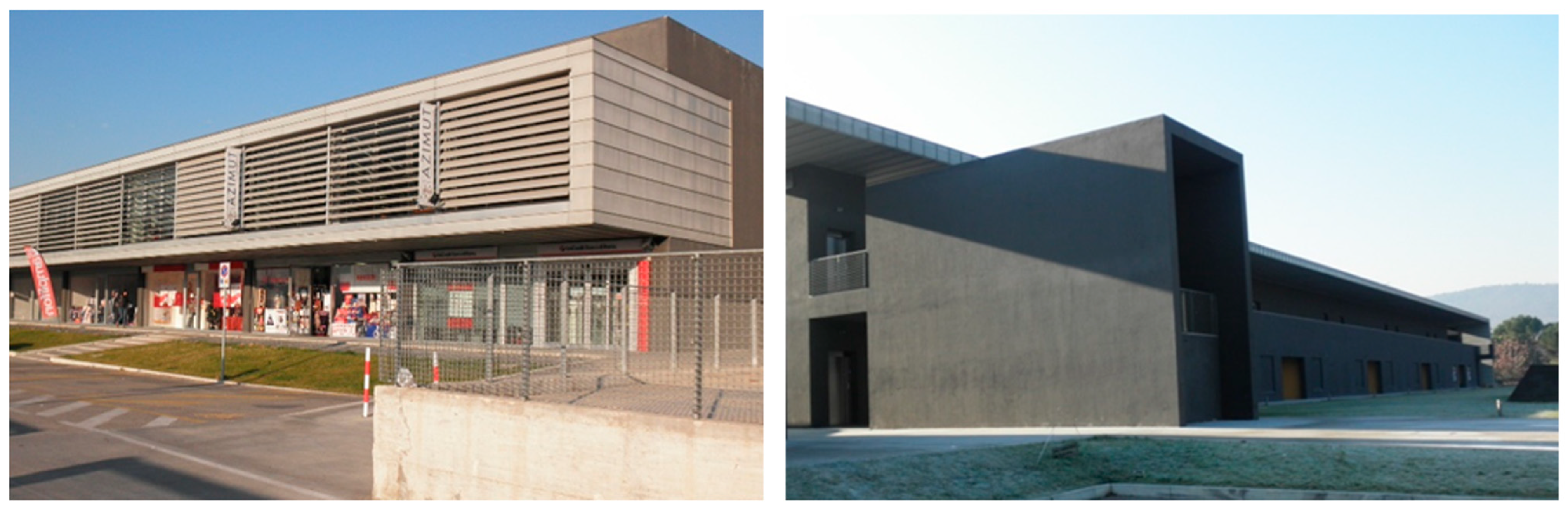
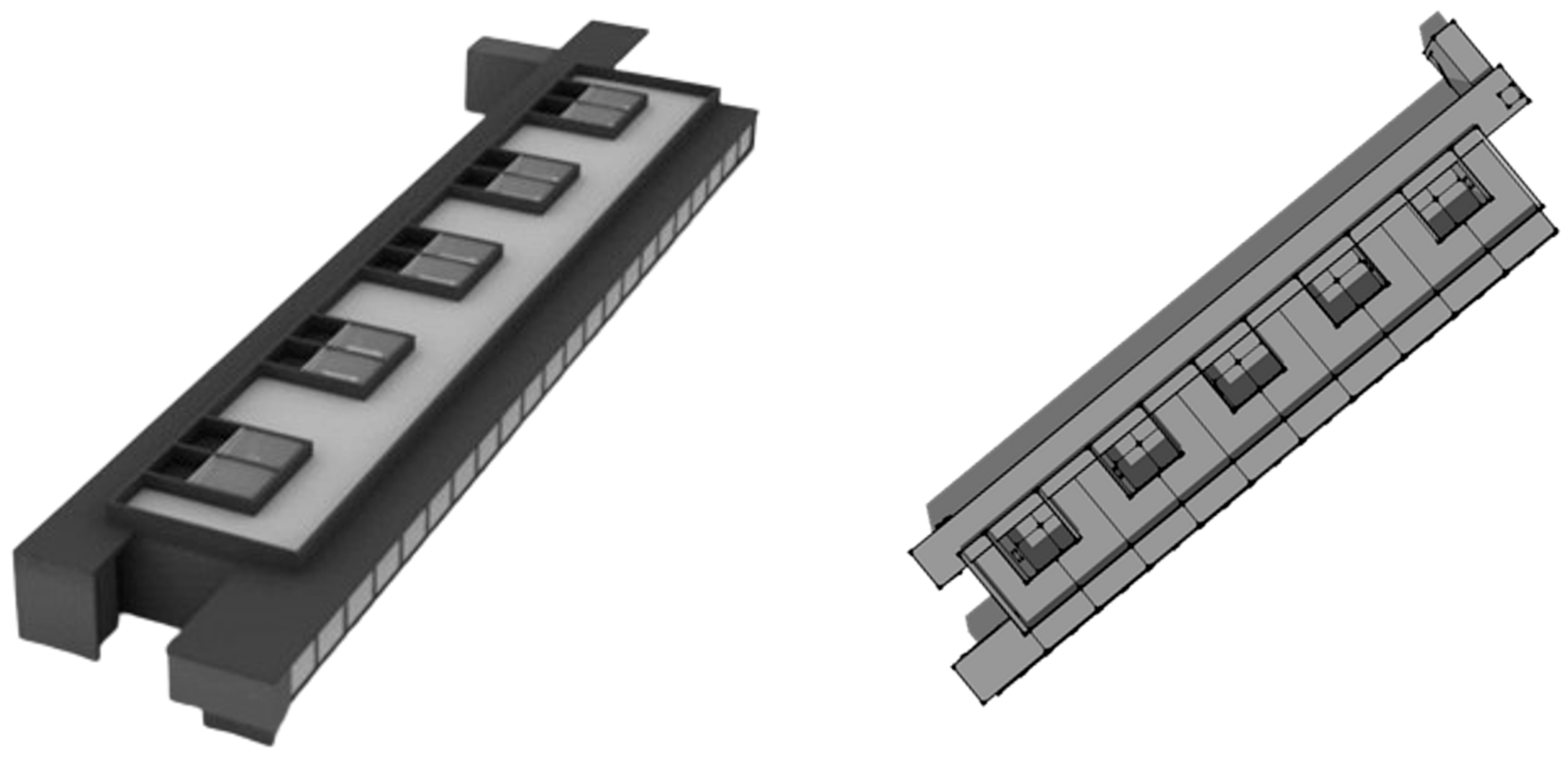
2.2. Case Study Description and the EnergyPlus Model
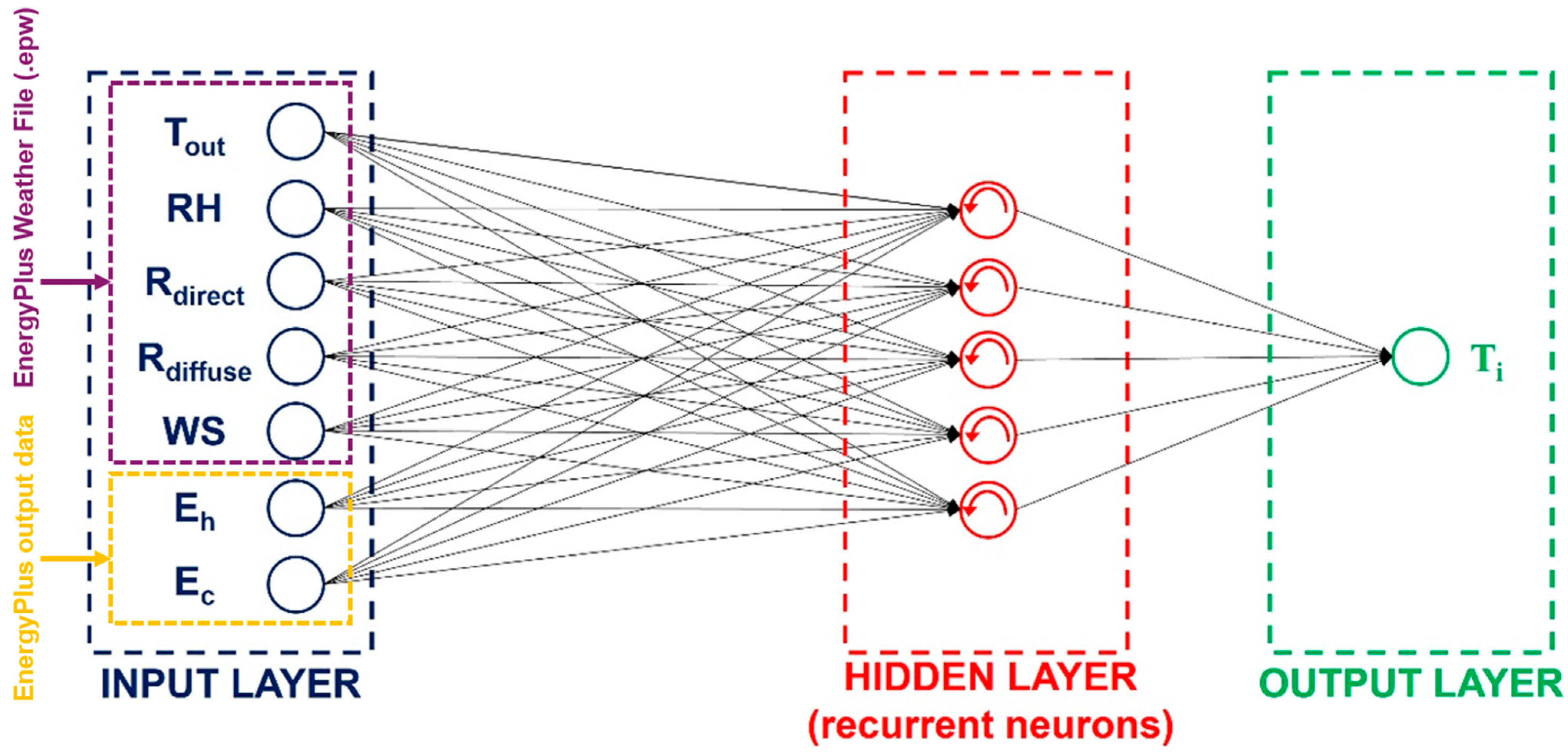
The commercial building chosen as the case study was built in 2005 in a suburb zone in central Italy (Figure 2). It consists of two floors, each one including five zones. The total height of the building is more than 10 m. The east and west facades are small and without windows; very large glass walls (with a total area of about 25 m2 for every zone) are in the south facades: they are provided with sunshades that can be used at peak hours. The facades of the ground floor are partially shaded by the upper floor, and an arcade is present in front of the commercial activities. The thermal transmittance of the opaque envelope is very low (0.25 W/(m2K)), and the total area of the activities (shops, coffee, restaurants, etc.) is about 600 m2. The first floor of the building presents 5 offices with an L-shaped plant (total floor area of 80 m2). Also, these rooms have large facades with southern exposure: the thermal transmittance of the double-glazed wall is 1.0 W/m2K. The mean window-to-wall (WWR) ratio of the rooms is 75%. The total inside volume of the building is about 12,000 m3 (considering both the offices and the shops), and the occupancy period chosen for all the final use is 8 a.m.–7 p.m. (except for the restaurant). Internal load contribution is about 6 W/m2 for offices and a mean value of 8 W/m2 for the shops/coffee bar.
The geometry of this building was implemented by means of the Google SketchUp plug-in, and the energy performances were evaluated by means of the E+ simulation code (Figure 3). EnergyPlus is able to model the building’s thermal performance, and the energy/electricity demands related to the HVAC system, equipment/plug loads, and lighting system. The inside vertical surfaces and the horizontal floor between the different zones allow for the transfer of heat, but they are at the same temperature as they are all air-conditioned. The external walls are considered to be heat exchanging surfaces with the outside boundary air conditions; also the ground floor can exchange heat with the soil. The room’s air set point temperature is fixed at 20 °C in the winter, and 26 °C in the summer periods.
Both opaque and transparent building envelope features are implemented in the E+ interface, where it is possible to specify the different layers that make up walls, ceilings, roofs, and floors. The thermal conductance, density, and heat capacity of each component can be included. The HVAC system features are also included in E+, where the peak power and efficiency of the heat pumps can be set for heating in terms of COP (coefficient of performance) and for cooling in terms of EER (energy efficiency ratio). The model also considers the lighting equipment; the number of LEDs and power are chosen to achieve 500 lumens per square meter inside the offices, and 300 lumens per square meter in the shop/coffee bar. The on/off switching periods have been set based on occupancy periods.
The building features (envelopes and plants) and occupancy schedules are the same in all the EnergyPlus simulations because the reference building is unique, and it should be consistent regardless of its location.
The energy demand for the maintenance of these temperatures inside the zones is calculated, and the corresponding electricity consumptions associated to a heat pump are evaluated in post-processing phases. The ON period in the winter season is not the same for all the selected Italian cities; the national limits are fixed based on the climatic classification of each location, and they are shown in Table 1.

2.3. RNN Model

The nonlinear functional relationship described by the thermoelectrical model of the building located was implemented through an RNN. The network architecture proposed is a network with recurrent hidden layers. This network implements internal feedback loops with variable delays, avoiding direct feedback between input and output. The architecture is defined by the number of hidden layers, the number of neurons for each layer, and the number of delays (i.e., states) for each layer.
With the goal of containing the computational costs associated with the neural estimator, a network with a single hidden layer was used, leaving the number of neurons and the number of delays as variable parameters. The same architecture for each climatic zone was used. For the training, 12 datasets, containing at each timestep the outside temperature (Tout), the relative humidity (RH), direct radiation (Rdirect), diffuse radiation (Rdiffuse), wind speed (WS), the mean inside air temperature at the beginning of the hour (Ti), the energy demand for heating (Eh), and the energy demand for cooling (Ec) are used in the implemented artificial neural network.
Each timestep corresponds to one hour of data. This temporal scale has been chosen because the start/stop schedules for the plants are generally programmed hour-by-hour. Furthermore, this timestep is commonly employed for monitoring the mean air temperatures and energy consumption of HVAC systems via smart meters. This could be useful for future applications of the model when real data is available.
The only data taken from the E+ program as input are related to the energy consumption for heating or cooling (Eh and Ec, respectively). The other input data are the environmental conditions, and they are taken from the EnergyPlus Weather Files (.epw) [55]. The output of the RNN is the hourly mean air temperatures of each building zone (Ti), for which the targets are obtained by the building simulation in E+. The input/output representation of the RNN is shown in Figure 4.
To determine the optimal size of the RNN in terms of hidden neurons and delay depth, an exhaustive test was performed by increasing progressively the hidden layer size and the delay depth, following the approach described in [57]. The optimal configuration of the RNN that yielded the best results in terms of fitting and generalization capabilities was represented by two delays and five neurons for the hidden layer. The RNN architecture and the most important training hyperparameters are reported in Table 2.
It is worth noting that each dataset, containing one year of hourly data, is divided monthly into twelve datasets, thus including several values equal to 672 (28 days for February), 720 (30 days for April, June, September, and November), and 744 (31 days for January, March, July, August, October, and December). Indeed, each neural network is trained and tested monthly to avoid temporal correlation between the data. Since each climatic zone is composed of four different cities and, therefore, by four databases, for each zone, one of them was used for testing the RNN, while the remaining three were used for the training. This test is provided to understand the RNN’s capabilities in a real scenario where training and deployment could happen for different climatic conditions. The performance metric is the RMSE calculated over each month. The algorithms of training and testing are implemented in the MATLAB r2024 environment, running on a 13th Gen Intel Core i9 CPU, with 32 GB of RAM [58].

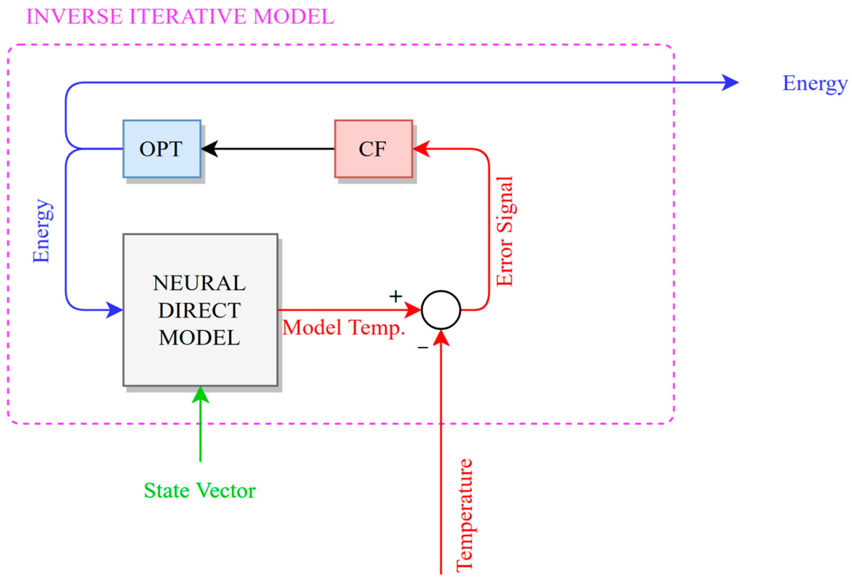
2.4. Model Inversion for REC Applications

The implemented neural model can be used to assess the thermal effects in the building for a known energetic input. However, to design HVAC controls, it is also useful to have an instrument able to estimate the energetic input necessary to achieve a specific thermal response. It is possible to define the direct problem as the determination of the thermal response from an energetic input, for a known “state vector” describing the environmental quantities of interest. The inverse problem then is the determination of the energetic demand for a known state vector, if a specific thermal response is required.
Such an inverse problem could be solved, in theory, simply by exchanging the inputs and outputs of the dataset, and thus training an RNN to solve the inverse problem. However, this approach required a large RNN, and proved very poor in terms of generalization capabilities. A different approach consists of posing the problem of determining the energetic demand as an optimization problem, as shown in Figure 5. In this case the RNN model is implemented inside an inverse iterative loop featuring an optimization algorithm. The algorithm optimizes the energetic demand sent to the RNN direct model until the difference between the model temperature and the demanded temperature is minimal. In this context, the inverted model features as input the demanded temperature, and as output the required energetic demand. Previous research works [44,45,46] have proposed the application of both direct and inverse models of RNNs, with the ultimate goal of predicting energy/electrical consumption and using the resulting data to optimize the operation of renewable energy communities (RECs) incorporating those investigated buildings.

3. Results

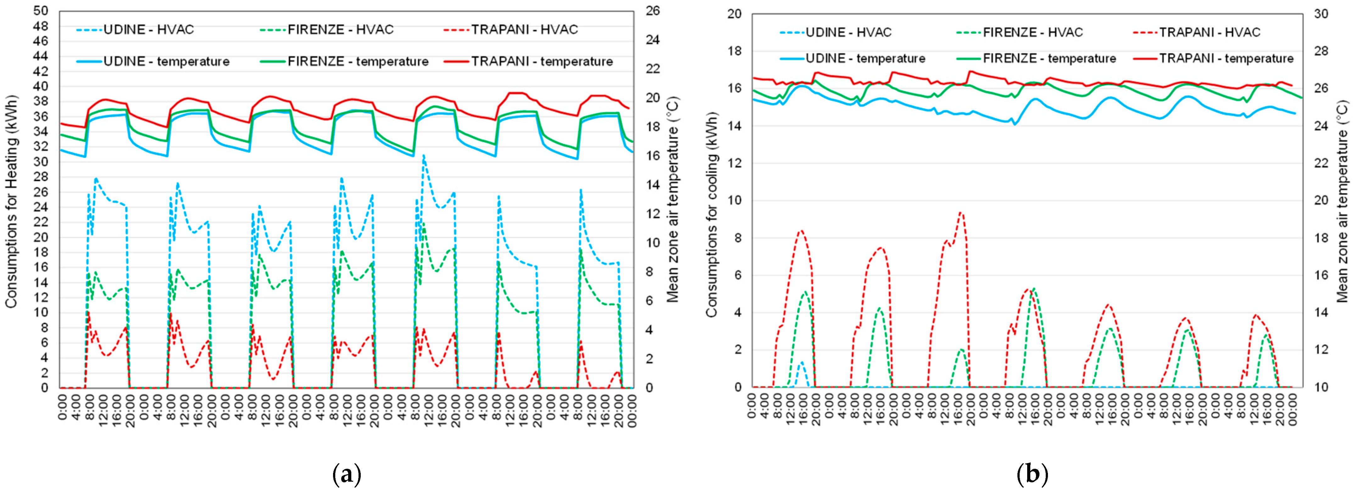
3.1. EnergyPlus Simulations Results

To find the Italian cities characterized from similar climatic conditions behavior, a preliminary analysis on their weather files was carried out in terms of monthly mean air temperatures and global solar radiation. As previously explained, three climatic zones were selected, typical of the north, central, and south regions of Italy. For each zone four cities were chosen, for a total number of twelve case studies.
The weather files used for the EnergyPlus simulation activities (EnergyPlus Weather data file [55]) used the mean data characteristics of every city that were averaged for about ten years, and they included hourly data for a total number of 8760 data (in particular, for mean air temperatures, for direct, diffuse, and global solar radiation, for relative humidity, and for mean air speed and direction). Figure 6a,b shows the comparison between the mean monthly data in terms of global solar radiation on horizontal surface and outdoor temperatures; it is possible to observe that the three climatic zones are clearly identifiable in the graph because the maximum solar radiation is always higher than 6000 Wh/m2 for the southern region, between 5000 and 6000 Wh/m2 for the central region, and about 5000 for the northern cities. For Bolzano, Trieste, Aviano, and Udine values lower than 1000 Wh/m2 are measured in the winter. For temperatures, Messina, Catania, Trapani, and Brindisi have values always higher than the other locations, and very similar to each other. Milano, Perugia, and Piacenza (central zone) also have similar trends, whereas Firenze has a behavior that can be compared with the northern locations and, in particular, it is very similar to Udine. More differences were observed for the northern cities above all in the winter months: Trieste has higher values comparable to central Italy, and both Aviano and Bolzano present air temperature values typical of mountain villages.
On the basis of these input data, yearly simulations were carried out considering the same case study situated in each of these cities with the on/off profiles of the plants specified in Table 1. A typical weekly behavior in December and in August is analyzed in Figure 7a,b for the three Italian zones in terms of indoor air temperatures and hourly electricity consumptions (kWh) required for the maintenance of the design air temperature values in winter (20 °C) and summer (26 °C). It is possible to observe that, in winter, to maintain the temperature between 19 °C and 21 °C, the heating consumptions in Udine are approximately twice the ones of Firenze (Figure 7a). Very low energy consumptions for heating are obtained in Trapani, mostly in the last two days when the outside air temperatures are high in southern Italy. It is important to observe two peak values of electricity consumption at the beginning and at the end of the heating period due to the solar radiation contribution during the central hours of the day: the large glazing façade with southern exposure allows the entry of heat and natural light. In the summer (Figure 7b), the hourly cooling consumptions are very low during the winter: maximum peak values of 8–10 kWh were obtained for Trapani, and for Firenze the maintenance of a temperature lower than 26 °C can be obtained with very low consumption (maximum values of 2–5 kWh). Finally, in Udine, the mean zone air temperatures are never higher than 26 °C, and for the whole week it is not necessary to turn on the plant (except for the first day).

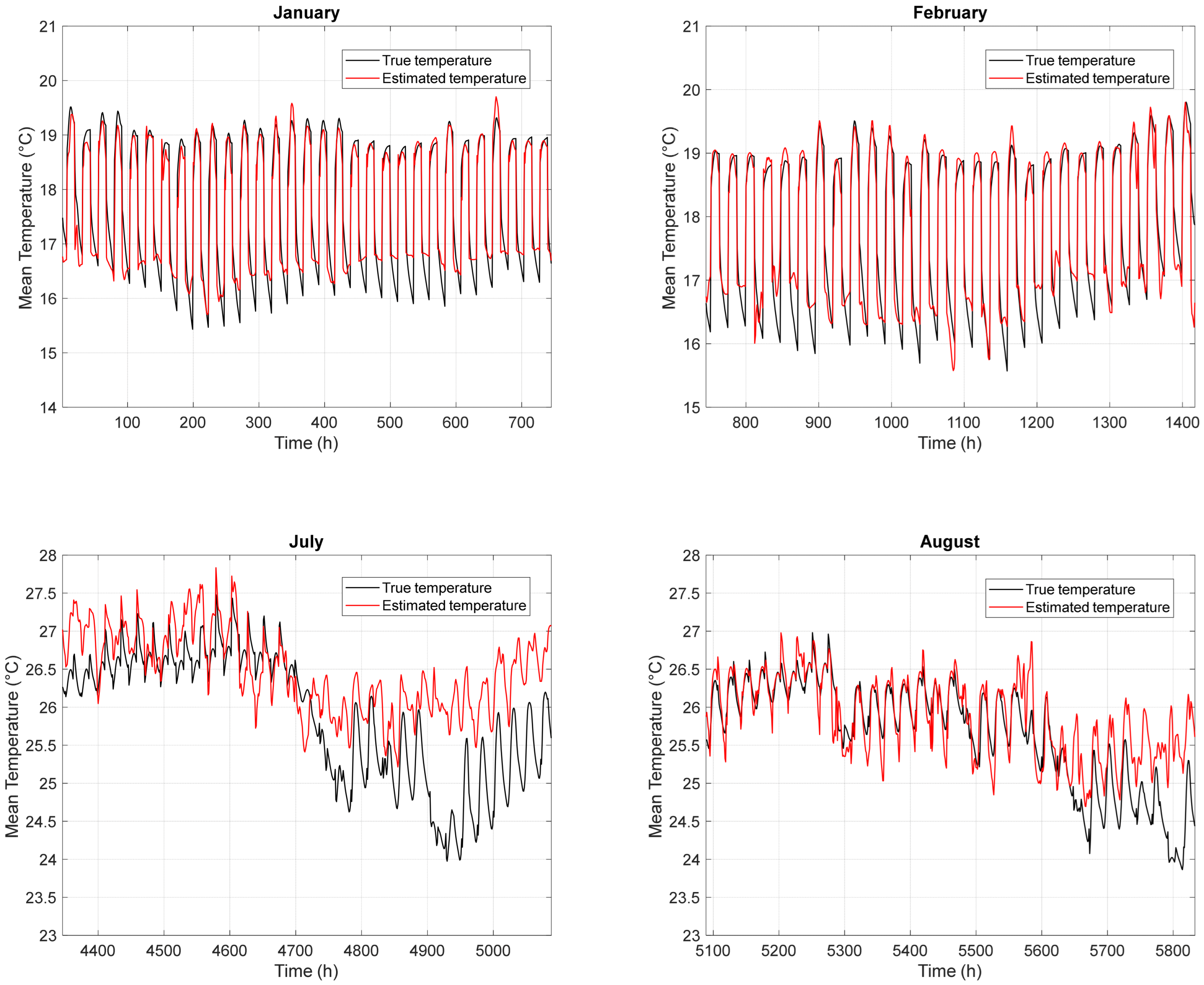
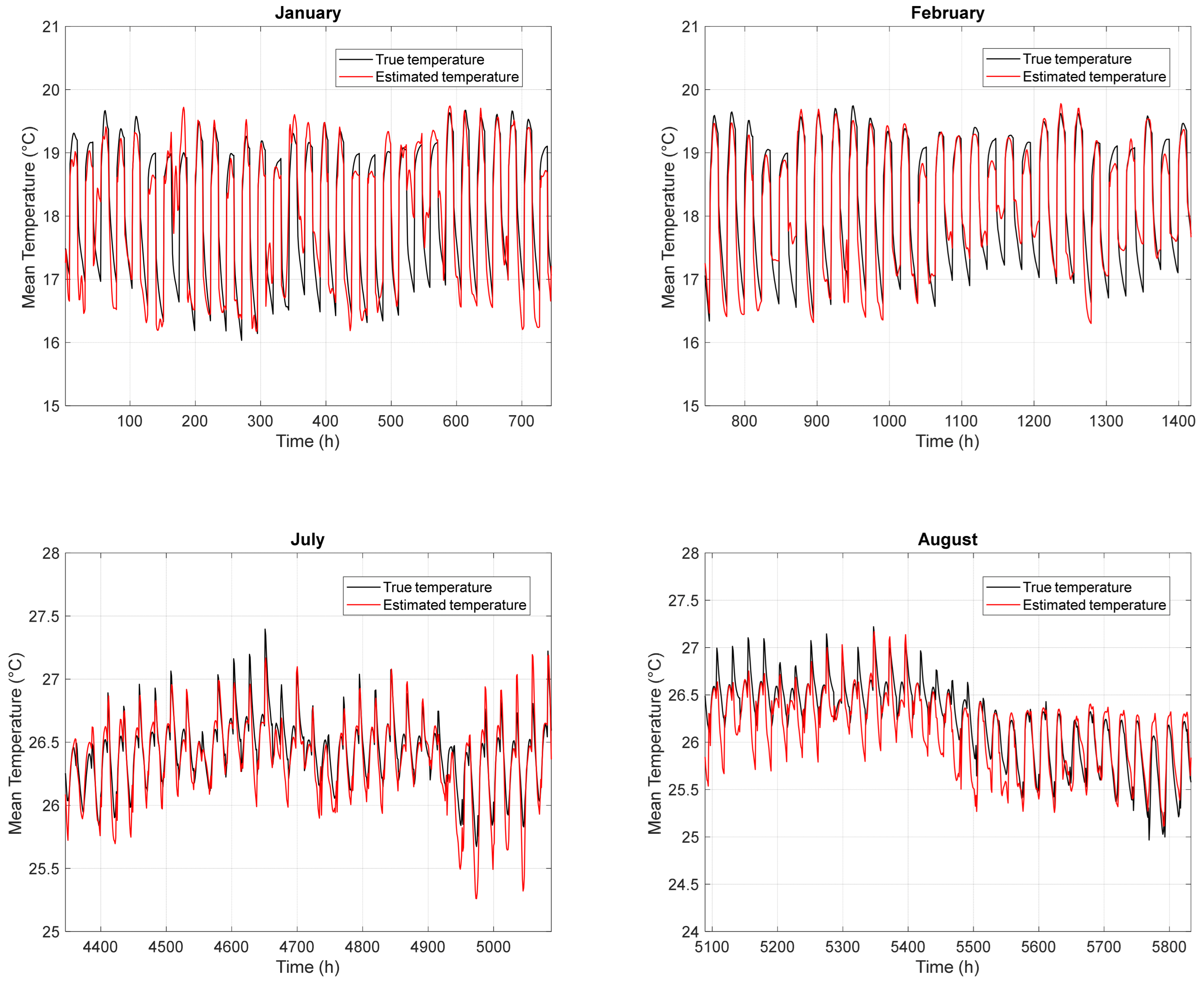
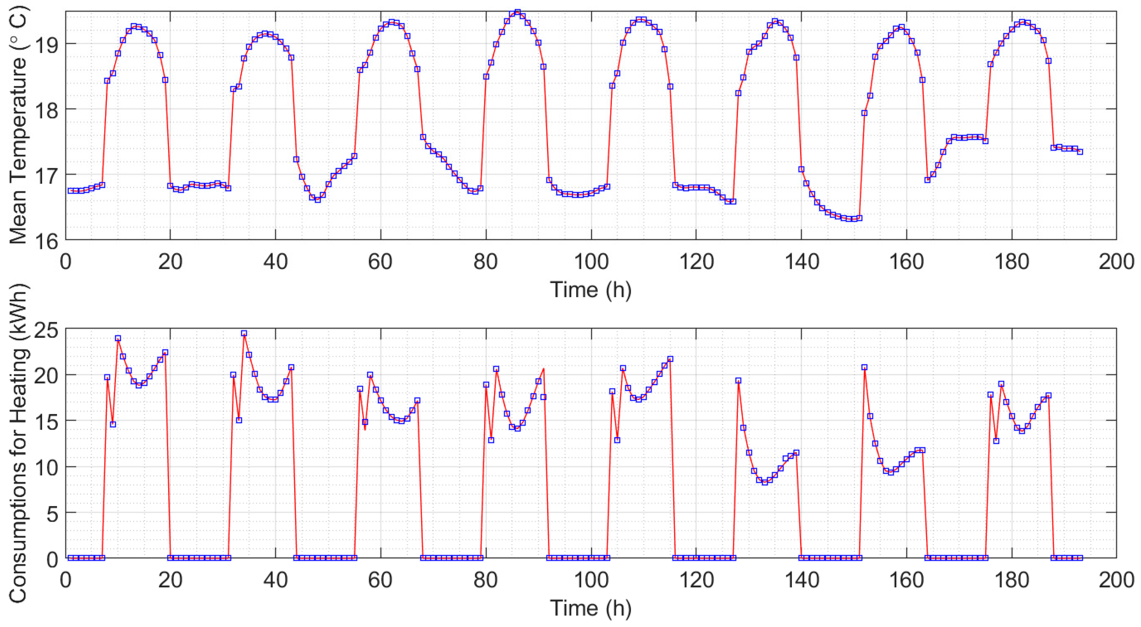
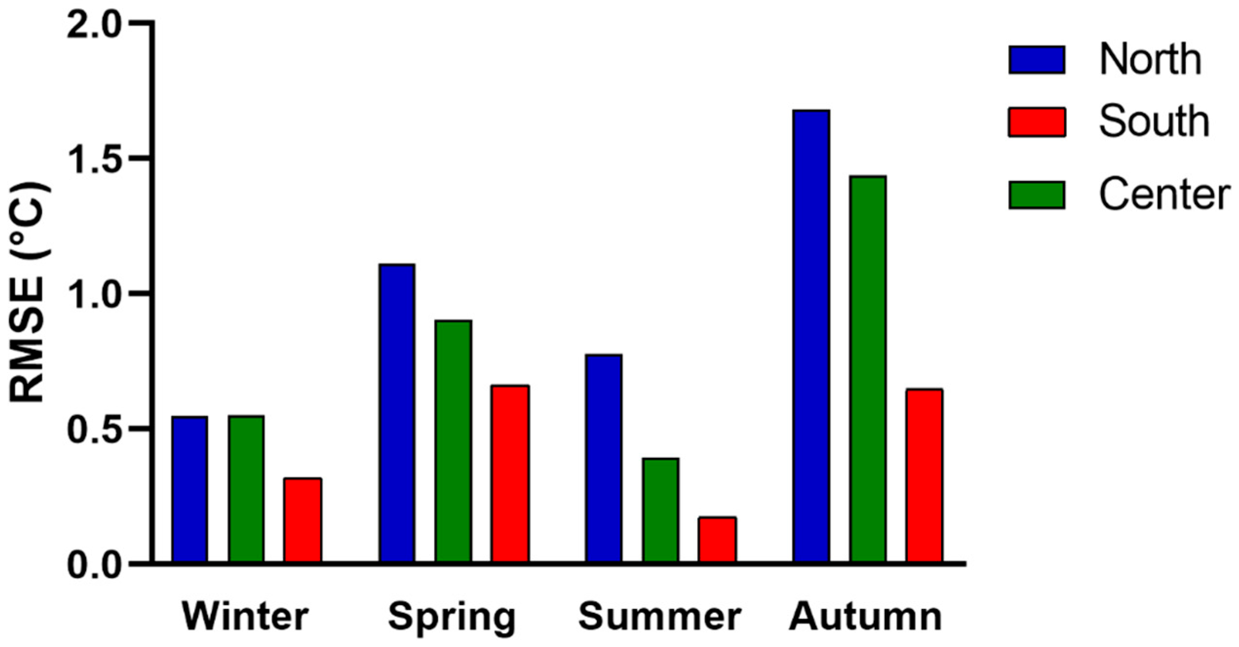
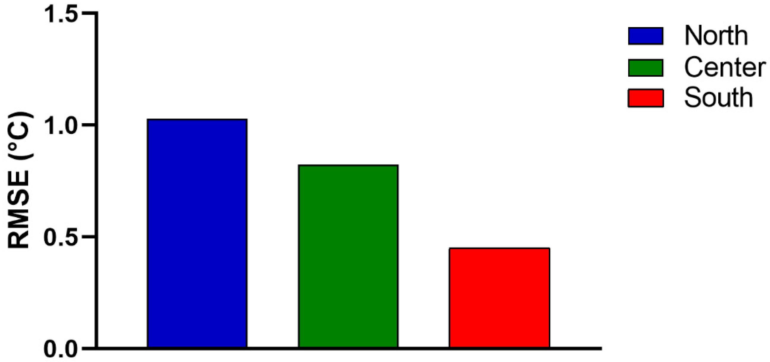
3.2. RNN Model Validation and Results

As mentioned above, for each one of the three climatic zones, four different RNN training sessions were performed using a dataset consisting of three cities. Every training session was tested using the fourth remaining city. Figure 8, Figure 9 and Figure 10 show the results of the predicted mean inside air temperature, Ti, for the three cities (Udine, Firenze, and Catania) that best represent the thermal behavior of the commercial buildings located in the north, center, and south of Italy, respectively. The mean inside-air temperatures trends are shown for two winter and summer months, i.e., January–February and July–August (the periods when the heating or the cooling systems are fully operational are chosen to avoid the mean-seasons when the building may require both heating and cooling depending on the outdoor weather conditions).
In general, it is possible to note that the trend of the estimated Ti is quite similar to the true one, for the three representative cities, showing good performance of the network in terms of being able to generalize towards new city climate conditions. However, a greater deviation is observed between the estimated and true temperatures in Udine during the summer months, because the training cities exhibited higher temperatures during the same months. Specifically, the maximum difference between the estimated and the true temperatures is less than 2 °C. This behavior is clearly an outlier, probably due to the lack of data on mean air temperature for this location in the north. This discrepancy highlights the limitations of the RNN during certain periods of the year.
For the remaining cities of each climatic zone (Aviano–Bolzano–Trieste, Milano–Perugia–Piacenza, Messina–Brindisi–Trapani), the average monthly RMSE was calculated, and the results are reported in Figure 11, Figure 12 and Figure 13. The tested RNN can predict the thermo-electrical behavior of the commercial buildings, exhibiting better results for the winter and summer months, i.e., when the heating and cooling systems were activated at full load. This result is pivotal in the smart management of energy aimed at reducing as much energy wastage as possible. For the mid-season, the figures show that, in the spring and autumn months, the average RMSE is higher than in the other months. In detail, for the northern climatic zone, it is lower than 6 °C, while for the central zone it is lower than 4 °C. Finally, for the southern climatic zone, it is lower than 2 °C. In these periods, the climatic conditions are highly variable in the Italian territory, and neighboring cities can also present different behaviors, especially in recent years where the climate changes have been most frequent. To obtain a better RNN performance during the spring and autumn seasons, it would be useful to consider a higher number of cities for each climatic zone.
Finally, the model inversion was tested on a small subset of the dataset to show the accuracy of the reconstructed energy profile using, as an optimization algorithm, the standard non-linear least square solver implemented in MATLAB. Over a period of 8 winter days, the inverted model reconstructed the energy profile with an RMSE of 0.31 Wh. The reconstructed profiles are shown in Figure 14. As can be seen, the model can be inverted without problems through a suitable optimization algorithm.

4. Critical Discussion

To comprehensively evaluate the neural network’s ability to predict internal temperatures that ensure thermal comfort, especially during the winter and summer, final performance metrics were calculated on a seasonal and annual basis. Specifically, Figure 15 reports the average root mean square error (RMSE) across the four seasons for each climatic zone.
As expected, the winter and summer seasons exhibit the best performance with an overall RMSE lower than 1 °C. This is predictable, as heating and cooling systems are primarily used during the winter and summer months, respectively. During the mid-seasons, the need for heating or cooling varies from day to day. Consequently, the neural network performs better in identifying the internal thermo-electric relationship precisely in those periods in which it is possible to control the internal temperature of the rooms by consciously switching the heating and cooling systems on and off. During the transitional seasons, the contribution of the energy demand of thermal systems is less significant. Therefore, the internal temperature of the site is primarily dependent on weather conditions and location. It is important to note that, in the southern regions, the RMSE is less than 0.7–0.8 °C, even in the summer and spring, due to the stable climatic conditions. The climate in the winter is also very mild and consistent throughout the year. The maximum error value is approximately 1.65 °C for the northern cities during the autumn. There are significant temperature fluctuations throughout the day, and users tend to turn off their plants for extended periods.
The average annual RMSE was then computed for each climate zone, as depicted in Figure 16. This allows for a direct comparison between the southern and northern climatic zones, indicating superior prediction accuracy in the former and less accurate predictions in the latter. This discrepancy could be attributed to more uniform occupant behavior in southern urban areas and a more diverse pattern of user activity in the northern regions, potentially influenced by greater climatic variability. Notably, the overall prediction error does not exceed 1 °C.

5. Limitations, Potential, and Future Works

Possible extensions of this work include exploring alternative sources of reference data or adopting different algorithmic implementations. In the first case, real-world experimental data could be used to train the artificial neural network (ANN). This approach has been adopted in previous studies, such as [50], where experimental measurements were collected from an educational building to train both direct and inverse ANN models. These models were then employed to simulate and optimize the operation of a renewable energy community (REC). In that study, environmental data from weather stations and energy consumption data from smart meters were used as ANN inputs, enabling the estimation of the mean indoor air temperature. For the inverse model, accurate hourly values of indoor temperature are required to estimate the corresponding energy consumption. This methodology, however, presents certain limitations. Simulation tools, such as EnergyPlus, allow for the same case study to be analyzed under different geographic and environmental conditions (a flexibility not afforded by the monitoring of a single real-world case). Therefore, a combined approach using both simulation data and ANN models provides enhanced versatility, as it requires only the outdoor environmental boundary conditions available in standard weather files for different locations. In future work, the authors intend to incorporate real data from non-residential buildings (including commercial, public, and industrial facilities), considering various boundary conditions (such as occupancy schedules and HVAC system operation). The analysis will also be extended to include additional geographic locations.
In the case of Italy, the national classification of climatic zones (six zones, from A to F) has been considered [59]. This classification defines the permitted heating and cooling periods for buildings during summer and winter, depending on the specific thermal needs of each zone. Twelve cities were selected, with four from each zone, to train three recurrent neural networks (RNNs), one for each major climatic area in Italy. This methodology can also be extended to other countries, as the input data required for the ANNs consists of outdoor environmental conditions (including mean air temperature, global solar radiation, relative humidity, and wind speed) and electrical consumption data related to heating or cooling. These data can be measured, collected, or derived from meteorological datasets available for other countries. In such cases, it is also possible to group cities from different countries that exhibit similar climatic characteristics. Regarding future development and application, the proposed framework could be scaled up for use across a national building stock or integrated into energy planning at the policy level. Since each building is characterized by specific thermal, electrical, and energy-related properties, the method can only be generalized by applying it to a sufficiently large number of buildings with similar characteristics (such as year of construction, thermal transmittance of opaque and transparent envelope components, and HVAC system specifications). Buildings with comparable features could be grouped together to represent segments of the building stock, and RNNs could be trained and implemented to analyze the behavior of each group. This approach could prove useful for forecasting the energy and electrical performance of representative buildings in each territory, as well as in the context of renewable energy community (REC) scenarios.
An additional consideration for future development concerns the structure and implementation potential of the proposed RNN models. Like neural models, RNNs are inherently scalable and can be extended to include additional input variables if required by specific applications or scenarios. Although the current implementation does not incorporate long-term memory, this limitation can be easily addressed by adopting more advanced architecture, such as long short-term memory (LSTM) or gated recurrent unit (GRU) networks, which are well-suited for capturing temporal dependencies over longer horizons [60,61].
Furthermore, due to their relatively low computational complexity and lightweight design, the proposed RNN models are well-suited for deployment on microcontroller-based systems that support TinyML frameworks, such as STMicroelectronics platforms [62,63]. This feature will be explored in future work with the goal of embedding models in edge devices for building automation. Such integration is particularly relevant in the context of smart buildings and intelligent energy management systems, where on-device inference enables real-time, energy-efficient operation without reliance on cloud-based infrastructure.

6. Conclusions

In Italy, non-residential buildings consume a significant amount of energy for heating/cooling, lighting, and other appliances due to their inadequate construction characteristics, which do not meet current legislative requirements. This is particularly true for buildings that are at least 20 years old. The present paper presents an interesting approach to model the relationship between thermal and energy demand in HVAC systems in different Italian locations. A commercial/office building was chosen as a case study, every feature of the building envelopes and plants were known, and it was modelled in the EnergyPlus program. Yearly simulations were carried out for twelve Italian cities, distributed evenly across the north, center, and south. Three artificial recurrent neural networks were developed based on the E+ output data: the first one was trained with the simulation results of the northern cities in Italy; the second was related to the behavior of the same building in central Italy; the third was suitable for the southern regions. The hourly electricity consumptions obtained for the occupancy periods were used as input in the RNN, and the temperature profiles of each zone are obtained as output. The monthly evaluation of the root mean square error reveals consistently low values, particularly during the winter and summer when the heating and cooling systems are activated in a distinct on–off manner. In this case the values are always lower than 1 °C. The RNN for the south also performs well in intermediate seasons when it is often necessary for the activation of the heat pumps in cooling mode or when the air conditioning is nowhere required. For the northern regions, the values of the seasonal RMSE are high above all for autumn (higher than 1.5 °C) when no specific trend for managing the plant has been identified. Future work could enhance the RNN model by incorporating data from additional Italian cities that represent the country’s diverse climatic zones. Furthermore, the inversion of the RNNs is being explored to predict electricity consumption (output) based on user temperature profiles (input). This inversion would enable the minimization of electricity loads by adjusting indoor thermal conditions (e.g., different target temperatures and operational schedules). This approach has promising applications, such as load dispatch optimization and building automation systems within smart grids and renewable energy communities.

Author Contributions

Conceptualization, G.M.L. and F.R.F.; methodology, G.M.L. and E.B.; software, M.P., M.Q. and F.F.; validation, E.B., M.P., M.Q. and F.F.; formal analysis, E.B. and G.M.L.; investigation, E.B. and G.M.L.; resources, F.R.F.; data curation, E.B., M.P. and G.M.L.; writing—original draft preparation, E.B., M.P., F.F. and G.M.L.; writing—review and editing, F.R.F. and M.Q.; visualization, E.B. and G.M.L.; supervision, F.R.F. and G.M.L.; project administration, F.R.F.; funding acquisition, F.R.F. All authors have read and agreed to the published version of the manuscript.

Funding

This study was carried out within the “Innovative Solutions for Renewables in Energy Communities (ISoREC)” project n. 202054TZLF—funded by European Union within the PRIN 2020 program (D.D. 1628—16/10/2020 Ministero dell’Università e della Ricerca—CUP: J57G20000100008). This manuscript reflects only the authors’ views and opinions, and the Ministry cannot be considered responsible for them.

Data Availability Statement

Data will be made available on request.

Conflicts of Interest

The authors declare no conflicts of interest.

References

  1. U.S. Department of Energy. Grid-Interactive Efficient Buildings Technical Report Series Overview of Research Challenges and Gaps. December 2019. Available online: https://www.energy.gov/eere/buildings/articles/grid-interactive-efficient-buildings-technical-report-series-overview (accessed on 3 April 2025).
  2. Martirano, L.; Rotondo, S. Modello di Microgrid per “Smart Building” Come Energy Community Con Gestione Ottimizzata Delle Risorse Energetiche Parte 1—Analisi di Modelli di Reti Energetiche per Smart Building e NZEB. Ricerca del Sistema Elettrico (RSE) e ENEA. Available online: https://www.ricercasistemaelettrico.enea.it/archivio-documenti/category/490-report-2019-progetto-1-5.html (accessed on 14 April 2025). (In Italian).
  3. Household Energy Consumption by Energy in the EU. Available online: https://www.odyssee-mure.eu/publications/efficiency-by-sector/households/energy-consumption-eu.html (accessed on 3 April 2025).
  4. Ding, C.; Ke, J.; Levine, M.; Zhou, N. Potential of artificial intelligence in reducing energy and carbon emissions of commercial buildings at scale. Nat. Commun. 2024, 15, 5916. [Google Scholar] [CrossRef] [PubMed]
  5. Brhane, G.Y.; Oh, E.; Son, S.Y. Virtual Energy Storage System Scheduling for Commercial Buildings with Fixed and Dynamic Energy Storage. Energies 2024, 17, 3292. [Google Scholar] [CrossRef]
  6. Rahman, A.; Srikumar, V.; Smith, A.D. Predicting electricity consumption for commercial and residential buildings using deep recurrent neural networks. Appl. Energy 2018, 212, 372–385. [Google Scholar] [CrossRef]
  7. Mocanu, E.; Nguyen, P.H.; Gibescu, M.; Kling, W.L. Deep learning for estimating building energy consumption. Sustain. Energy Grids Netw. 2016, 6, 91–99. [Google Scholar] [CrossRef]
  8. Robinson, C.; Dilkina, B.; Hubbs, J.; Zhang, W.; Guhathakurta, S.; Brown, M.A.; Pendyala, R.M. Machine learning approaches for estimating commercial building energy consumption. Appl. Energy 2017, 208, 889–904. [Google Scholar] [CrossRef]
  9. Michailidis, P.; Michailidis, I.; Gkelios, S.; Kosmatopoulos, E. Artificial Neural Network Applications for Energy Management in Buildings: Current Trends and Future Directions. Energies 2024, 17, 570. [Google Scholar] [CrossRef]
  10. Chitalia, G.; Pipattanasomporn, M.; Garg, V.; Rahman, S. Robust short-term electrical load forecasting framework for commercial buildings using deep recurrent neural networks. Appl. Energy 2020, 278, 115410. [Google Scholar] [CrossRef]
  11. Huang, H.; Chen, L.; Hu, E. A neural network-based multi-zone modelling approach for predictive control system design in commercial buildings. Energy Build. 2015, 97, 86–97. [Google Scholar] [CrossRef]
  12. Fu, H.; Baltazar, J.C.; Claridge, D.E. Review of developments in whole-building statistical energy consumption models for commercial buildings. Renew. Sustain. Energy Rev. 2021, 147, 111248. [Google Scholar] [CrossRef]
  13. Macarulla, M.; Casals, M.; Forcada, N.; Gangolells, M. Implementation of predictive control in a commercial building energy management system using neural networks. Energy Build. 2017, 151, 511–519. [Google Scholar] [CrossRef]
  14. Afzal, S.; Shokri, A.; Ziapour, B.M.; Shakibi, H.; Sobhani, B. Building energy consumption prediction and optimization using different neural network-assisted models; comparison of different networks and optimization algorithms. Energy 2023, 282, 128446. [Google Scholar] [CrossRef]
  15. Han, Y.; Fan, C.; Geng, Z.; Ma, B.; Cong, D.; Chen, K.; Yu, B. Energy efficient building envelope using novel RBF neural network integrated affinity propagation. Energy 2020, 209, 118414. [Google Scholar] [CrossRef]
  16. Severiche-Maury, Z.; Uc-Rios, C.E.; Arrubla-Hoyos, W.; Cama-Pinto, D.; Holgado-Terriza, J.A.; Damas-Hermoso, M.; Cama-Pinto, A. Forecasting Residential Energy Consumption with the Use of Long Short-Term Memory Recurrent Neural Networks. Energies 2025, 18, 1247. [Google Scholar] [CrossRef]
  17. Uba, F.; Apevienyeku, H.K.; Nsiah, F.D.; Akorli, A.; Adjignon, S. Energy Analysis of Commercial Buildings Using Artificial Neural Network. Model. Simul. Eng. 2021, 2021, 8897443. [Google Scholar] [CrossRef]
  18. Genkin, M.; McArthur, J.J. B-SMART: A reference architecture for artificially intelligent autonomic smart buildings. Eng. Appl. Artif. Intell. 2023, 121, 106063. [Google Scholar] [CrossRef]
  19. Kulathilaka, M.J.S.; Saravanan, S.; Kumarasiri, H.D.H.P.; Logeeshan, V.; Kumarawadu, S.; Wanigasekara, C. NILM for Commercial Buildings: Deep Neural Networks Tackling Nonlinear and Multi-Phase Loads. Energies 2024, 17, 3802. [Google Scholar] [CrossRef]
  20. Lu, Y.; Chen, Q.; Yu, M.; Wu, Z.; Huang, C.; Fu, J.; Yu, Z.; Yao, J. Exploring spatial and environmental heterogeneity affecting energy consumption in commercial buildings using machine learning. Sustain. Cities Soc. 2023, 95, 104586. [Google Scholar] [CrossRef]
  21. Liang, W.; Li, H.; Zhan, S.; Chong, A.; Hong, T. Energy flexibility quantification of a tropical net-zero office building using physically consistent neural network-based model predictive control. Adv. Appl. Energy 2024, 14, 100167. [Google Scholar] [CrossRef]
  22. Han, F.; Du, F.; Jiao, S.; Zou, K. Predictive Analysis of a Building’s Power Consumption Based on Digital Twin Platforms. Energies 2024, 17, 3692. [Google Scholar] [CrossRef]
  23. Gao, Z.; Yang, S.; Yu, J.; Zhao, A. Hybrid forecasting model of building cooling load based on combined neural network. Energy 2024, 297, 131317. [Google Scholar] [CrossRef]
  24. Jiang, B.; Li, Y.; Rezgui, Y.; Zhang, C.; Wang, P.; Zhao, T. Multi-source domain generalization deep neural network model for predicting energy consumption in multiple office buildings. Energy 2024, 299, 131467. [Google Scholar] [CrossRef]
  25. Ye, H.; Zhu, Q.; Zhang, X. Short-Term Load Forecasting for Residential Buildings Based on Multivariate Variational Mode Decomposition and Temporal Fusion Transformer. Energies 2024, 17, 3061. [Google Scholar] [CrossRef]
  26. Wang, G.; Mukhtar, A.; Moayedi, H.; Khalilpoor, N.; Tt, Q. Application and evaluation of the evolutionary algorithms combined with conventional neural network to determine the building energy consumption of the residential sector. Energy 2024, 298, 131312. [Google Scholar] [CrossRef]
  27. Biswas, M.A.R.; Robinson, M.D.; Fumo, N. Prediction of residential building energy consumption: A neural network approach. Energy 2016, 117 Pt 1, 84–92. [Google Scholar] [CrossRef]
  28. Li, T.; Liu, X.; Li, G.; Wang, X.; Ma, J.; Xu, C.; Mao, Q. A systematic review and comprehensive analysis of building occupancy prediction. Renew. Sustain. Energy Rev. 2024, 193, 114284. [Google Scholar] [CrossRef]
  29. Azar, E.; O’Brien, W.; Carlucci, S.; Hong, T.; Sonta, A.; Kim, J.; Andargie, M.S.; Abuimara, T.; Asmar, M.E.; Jain, R.K.; et al. Simulation-aided occupant-centric building design: A critical review of tools, methods, and applications. Energy Build. 2020, 224, 110292. [Google Scholar] [CrossRef]
  30. Li, T.; Liu, X.; Zhou, W.; Ma, J.; Li, Y.; Gao, J.; Chen, M.; Mao, Q. Optimizing building energy consumption through synchronization and asynchronization of occupancy and air-conditioning behavior. Energy Build. 2025, 331, 115409. [Google Scholar] [CrossRef]
  31. Wang, X.; Li, T.; Yu, Y.; Liu, Q.; Shi, L.; Xia, J.; Mao, Q. Performance simulation and energy efficiency analysis of multi-energy complementary HVAC system based on TRNSYS. Appl. Therm. Eng. 2024, 257 Pt B, 124378. [Google Scholar] [CrossRef]
  32. Nutakki, M.; Mandava, S. Review on optimization techniques and role of Artificial Intelligence in home energy management systems. Eng. Appl. Artif. Intell. 2023, 119, 105721. [Google Scholar] [CrossRef]
  33. Khalil, M.; McGough, A.S.; Pourmirza, Z.; Pazhoohesh, M.; Walker, S. Machine Learning, Deep Learning and Statistical Analysis for forecasting building energy consumption—A systematic review. Eng. Appl. Artif. Intell. 2022, 115, 105287. [Google Scholar] [CrossRef]
  34. Mehmood, M.U.; Chun, D.; Zeeshan; Han, H.; Jeon, G.; Chen, K. A review of the applications of artificial intelligence and big data to buildings for energy-efficiency and a comfortable indoor living environment. Energy Build. 2019, 202, 109383. [Google Scholar] [CrossRef]
  35. EnergyPlus Program, 23.2.0 Version. Available online: https://energyplus.net/ (accessed on 14 April 2025).
  36. Chung, W.J.; Liu, C. Analysis of input parameters for deep learning-based load prediction for office buildings in different climate zones using eXplainable Artificial Intelligence. Energy Build. 2022, 276, 112521. [Google Scholar] [CrossRef]
  37. Si, B.; Wang, J.; Yao, X.; Shi, X.; Jin, X.; Zhou, X. Multi-objective optimization design of a complex building based on an artificial neural network and performance evaluation of algorithms. Adv. Eng. Inform. 2019, 40, 93–109. [Google Scholar] [CrossRef]
  38. Edwards, R.E.; New, J.; Parker, L.E.; Cui, B.; Dong, J. Constructing large scale surrogate models from big data and artificial intelligence. Appl. Energy 2017, 202, 685–699. [Google Scholar] [CrossRef]
  39. Wong, S.L.; Wan, K.K.W.; Tony, N.T.L. Artificial neural networks for energy analysis of office buildings with daylighting. Appl. Energy 2010, 87, 551–557. [Google Scholar] [CrossRef]
  40. Saryazdi, S.M.E.; Etemad, A.; Shafaat, A.; Bahman, A.M. Data-driven performance analysis of a residential building applying artificial neural network (ANN) and multi-objective genetic algorithm (GA). Build. Environ. 2022, 225, 109633. [Google Scholar] [CrossRef]
  41. Melo, A.P.; Cóstola, D.; Lamberts, R.; Hensen, J.L.M. Development of surrogate models using artificial neural network for building shell energy labelling. Energy Policy 2014, 69, 457–466. [Google Scholar] [CrossRef]
  42. Lazzeroni, P.; Mariuzzo, I.; Quercio, M.; Repetto, M. Economic, Energy, and Environmental Analysis of PV with Battery Storage for Italian Households. Electronics 2021, 10, 146. [Google Scholar] [CrossRef]
  43. Chou, J.S.; Bui, D.K. Modeling heating and cooling loads by artificial intelligence for energy-efficient building design. Energy Build. 2014, 82, 437–446. [Google Scholar] [CrossRef]
  44. Belloni, E.; Bianchini, G.; Casini, M.; Faba, A.; Intravaia, M.; Laudani, A.; Lozito, G.M. An overview on building-integrated photovoltaics: Technological solutions, modeling, and control. Energy Build. 2024, 324, 114867. [Google Scholar] [CrossRef]
  45. Lucaferri, V.; Quercio, M.; Laudani, A.; Riganti Fulginei, F. A Review on Battery Model-Based and Data-Driven Methods for Battery Management Systems. Energies 2023, 16, 7807. [Google Scholar] [CrossRef]
  46. Risi, B.; Riganti Fulginei, F.; Laudani, A.; Quercio, M. Compensation Admittance Load Flow: A Computational Tool for the Sustainability of the Electrical Grid. Sustainability 2023, 15, 14427. [Google Scholar] [CrossRef]
  47. Belloni, E.; Lozito, G.M.; Reatti, A. A Python Tool for Simulation and Optimal Sizing of a Storage Equipped Grid Connected Photovoltaic Power System. In Proceedings of the 2022 IEEE 21st Mediterranean Electrotechnical Conference (MELECON), Palermo, Italy, 14–16 June 2022; pp. 884–889. [Google Scholar] [CrossRef]
  48. Belloni, E.; Fulginei, F.R.; Lozito, G.M.; Poli, D. Direct and Inverse Neural Modelling of Buildings HVAC Systems. In Proceedings of the IEEE EUROCON 2023—20th International Conference on Smart Technologies, Torino, Italy, 6–8 July 2023; pp. 269–274. [Google Scholar] [CrossRef]
  49. Palermo, M.; Forconi, F.; Belloni, E.; Quercio, M.; Lozito, G.M.; Fulginei, F.R. Optimization of a feedforward neural network’s architecture for an HVAC system problem. In Proceedings of the 2023 3rd International Conference on Electrical, Computer, Communications and Mechatronics Engineering (ICECCME), Tenerife, Spain, 19–21 July 2023; pp. 1–6. [Google Scholar] [CrossRef]
  50. Belloni, E.; Grasso, F.; Lozito, G.M.; Poli, D.; Riganti Fulginei, F.; Talluri, G. Neural-assisted HVACs optimal scheduling for renewable energy communities. Energy Build. 2023, 301, 113658. [Google Scholar] [CrossRef]
  51. Liu, B.; Vu-Bac, N.; Zhuang, X.; Fu, X.; Rabczuk, T. Stochastic integrated machine learning based multiscale approach for the prediction of the thermal conductivity in carbon nanotube reinforced polymeric composites. Compos. Sci. Technol. 2022, 224, 109425. [Google Scholar] [CrossRef]
  52. Liu, B.; Vu-Bac, N.; Rabczuk, T. A stochastic multiscale method for the prediction of the thermal conductivity of Polymer nanocomposites through hybrid machine learning algorithms. Compos. Struct. 2021, 273, 114269. [Google Scholar] [CrossRef]
  53. Ji, J.; Yu, H.; Wang, X.; Xu, X. Machine learning application in building energy consumption prediction: A comprehensive review. J. Build. Eng. 2025, 104, 112295. [Google Scholar] [CrossRef]
  54. Liu, B.; Vu-Bac, N.; Zhuang, X.; Liu, W.; Fu, X.; Rabczuk, T. Al-DeMat: A web-based expert system platform for computationally expensive models in materials design. Adv. Eng. Softw. 2023, 176, 103398. [Google Scholar] [CrossRef]
  55. EnergyPlus Weather Data File. Available online: https://energyplus.net/weather (accessed on 14 April 2025).
  56. Buratti, C.; Moretti, E.; Belloni, E. Nanogel Windows for Energy Building Efficiency. In Nano and Biotech Based Materials for Energy Building Efficiency; Pacheco Torgal, F., Buratti, C., Kalaiselvam, S., Granqvist, C.G., Ivanov, V., Eds.; Springer: Cham, Switzerland, 2016. [Google Scholar] [CrossRef]
  57. Lozito, G.M.; Salvini, A. Swarm intelligence based approach for efficient training of regressive neural networks. Neural Comput. Appl. 2020, 32, 10693–10704. [Google Scholar] [CrossRef]
  58. MathWorks. MATLAB r2022. 2022. Available online: https://www.mathworks.com/products/new_products/release2022a.html (accessed on 3 April 2025).
  59. Regulation Containing Rules for the Design, Installation, Operation and Maintenance of Heating Systems in Buildings for the Purpose of Containing Energy Consumption. D.P.R 412/1993, Updated on 28 April 2022. Available online: https://www.normattiva.it/uri-res/N2Ls?urn:nir:stato:decreto.del.presidente.della.repubblica:1993-08-26;412!vig= (accessed on 14 April 2025).
  60. Somu, N.; MR, G.R.; Ramamritham, K. A deep learning framework for building energy consumption forecast. Renew. Sustain. Energy Rev. 2021, 137, 110591. [Google Scholar] [CrossRef]
  61. Mtibaa, F.; Nguyen, K.K.; Azam, M.; Papachristou, A.; Venne, J.S.; Cheriet, M. LSTM-based indoor air temperature prediction framework for HVAC systems in smart buildings. Neural Comput. Appl. 2020, 32, 17569–17585. [Google Scholar] [CrossRef]
  62. Osman, A.; Abid, U.; Gemma, L.; Perotto, M.; Brunelli, D. Tinyml platforms benchmarking. In Proceedings of the International Conference on Applications in Electronics Pervading Industry, Environment and Society, Online, 21–22 September 2021; Springer International Publishing: Cham, Switzerland, 2021; pp. 139–148. [Google Scholar]
  63. Sudharsan, B.; Salerno, S.; Nguyen, D.D.; Yahya, M.; Wahid, A.; Yadav, P.; Breslin, J.G.; Ali, M.I. TinyML benchmark: Executing fully connected neural networks on commodity microcontrollers. In Proceedings of the 2021 IEEE 7th World Forum on Internet of Things (WF-IoT), New Orleans, LA, USA, 14 June–31 July 2021; IEEE: Piscataway, NJ, USA; pp. 883–884. [Google Scholar]
Figure 1. Flowchart of the training set creation approach.
Energies 18 03031 g001
Figure 2. Front and back side of the commercial/office building.
Energies 18 03031 g002
Figure 3. 3D model of the building chosen as the case study.
Energies 18 03031 g003
Figure 4. Architecture of the RNN used for the thermo-electrical model of the commercial/office building.
Energies 18 03031 g004
Figure 5. Block diagram of the direct and inverse modes of operation of the algorithms.
Energies 18 03031 g005
Figure 6. Comparison between the monthly mean values in terms of solar radiation (a) and mean air temperature (b) obtained from the EnergyPlus weather files.
Energies 18 03031 g006
Figure 7. EnergyPlus simulation results in terms of indoor air temperature and electricity consumptions: (a) winter week; (b) summer week.
Energies 18 03031 g007
Figure 8. Prediction of the mean inside air temperature (Ti) in January, February, July, and August for Udine (northern Italy). The estimated temperature is represented by the red line, while the true temperature is represented by the black line.
Energies 18 03031 g008
Figure 9. Prediction of the mean inside air temperature (Ti) in January, February, July, and August for Firenze (central Italy). The estimated temperature is represented by the red line, while the true temperature is represented by the black line.
Energies 18 03031 g009
Figure 10. Prediction of the mean inside air temperature (Ti) in January, February, July, and August for Catania (southern Italy). The estimated temperature is represented by the red line, while the true temperature is represented by the black line.
Energies 18 03031 g010
Figure 11. Monthly average RMSE from January to June (a) and from July to December (b) for Aviano, Bolzano, and Trieste, representatives of the northern climatic zone.
Energies 18 03031 g011
Figure 12. Monthly average RMSE from January to June (a) and from July to December (b) for Milano, Perugia, and Piacenza, representatives of the central climatic zone.
Energies 18 03031 g012
Figure 13. Monthly average RMSE from January to June (a) and from July to December (b) for Messina, Brindisi, and Trapani, representatives of the southern climatic zone.
Energies 18 03031 g013
Figure 14. Results of the model inversion approach. (Bottom), the true energy demand (red curve) and the reconstructed energy demand (blue square). (Top), the reference temperature (red curve) and the temperature resulting from the reconstructed energy demand (blue square).
Energies 18 03031 g014
Figure 15. Seasonal average RMSE for the three climatic zones.
Energies 18 03031 g015
Figure 16. Annual average RMSE for the three climatic zones.
Energies 18 03031 g016
Table 1. Simulated case studies considered for the analysis and the ON-period of the HVAC.
NORTH
Climatic Zone 1
CENTER
Climatic Zone 2
SOUTH
Climatic Zone 3
Heating
Period
Cooling
Period
Heating
Period
Cooling
Period
Heating
Period
Cooling
Period
Annual ON
period
01/10–30/0401/07–15/0915/10–15/0401/06–30/0915/11–15/0301/05–15/10
Design
Temperatures
20 ± 1 °C26 ± 1 °C20 ± 1 °C26 ± 1 °C20 ± 1 °C26 ± 1 °C
Daily ON period8 a.m.–7 p.m.
Table 2. Summary of the RNN architecture and training hyperparameters.
ParameterValue or Description
ArchitectureLayer Recurrent Neural Network (layrecnet)
Number of Hidden Layers1
Activation FunctionTangent Sigmoid (tansig)
Feedback Delays2
Sample Time1
Total Number of Weights91
Training AlgorithmLevenberg–Marquardt (trainlm)
Performance MetricMean Squared Error (MSE)
Data DivisionRandom by sample (dividerand)
Training/Validation Split70%/30%
Maximum Training Epochs10.000
Minimum Gradient1 × 10−7
Maximum Validation Failures250
Average Training Time93 s
Average Inference Time4.4 ms
Average Epochs for Training1500–2000
Disclaimer/Publisher’s Note: The statements, opinions and data contained in all publications are solely those of the individual author(s) and contributor(s) and not of MDPI and/or the editor(s). MDPI and/or the editor(s) disclaim responsibility for any injury to people or property resulting from any ideas, methods, instructions or products referred to in the content.

