Thermal-Hydrologic-Mechanical Processes and Effects on Heat Transfer in Enhanced/Engineered Geothermal Systems

Abstract

Enhanced or engineered geothermal systems (EGSs), or non-hydrothermal resources, are highly notable among sustainable energy resources because of their abundance and cleanness. The EGS concept has received worldwide attention and undergone intensive studies in the last decade in the US and around the world. In comparison, hydrothermal reservoir resources, the ‘low-hanging fruit’ of geothermal energy, are very limited in amount or availability, while EGSs are extensive and have great potential to supply the entire world with the needed energy almost permanently. The EGS, in essence, is an engineered subsurface heat mining concept, where water or another suitable heat exchange fluid is injected into hot formations to extract heat from the hot dry rock (HDR). Specifically, the EGS relies on the principle that injected water, or another working fluid, penetrates deep into reservoirs through fractures or high-permeability channels to absorb large quantities of thermal energy by contact with the host hot rock. Finally, the heated fluid is produced through production wells for electricity generation or other usages. Heat mining from fractured EGS reservoirs is subject to complex interactions within the reservoir rock, involving high-temperature heat exchange, multi-phase flow, rock deformation, and chemical reactions under thermal-hydrological-mechanical (THM) processes or thermal-hydrological-mechanical-chemical (THMC) interactions. In this paper, we will present a THM model and reservoir simulator and its application for simulation of hydrothermal geothermal systems and EGS reservoirs as well as a methodology of coupling thermal, hydrological, and mechanical processes. A numerical approach, based on discretizing the thermo-poro-elastic Navier equation using an integral finite difference method, is discussed. This method provides a rigorous, accurate, and efficient fully coupled methodology for the three (THM) strongly interacted processes. Several programs based on this methodology are demonstrated in the simulation cases of geothermal reservoirs, including fracture aperture enhancement, thermal stress impact, and tracer transport in a field-scale reservoir. Results are displayed to show geomechanics’ impact on fluid and heat flow in geothermal reservoirs.

1. Introduction

Geothermal heat is one of the most promising renewable energy resources, but it has not been developed commercially on a large scale yet, because of both technical and economic issues. Continual research effort is still needed to better understand the engineering processes of geothermal reservoir development. Despite the progress made, it remains a challenge to numerically model fluid/heat flow in geothermal reservoirs due to the strongly coupled THM interactions. That is, when a cold working fluid is injected into the hot reservoir, fluid flow triggers the alteration in pore pressure, which leads to the geo-mechanical response that transforms the in situ stress field. Simultaneously, heat transfer occurring during convection and conduction exerts an impact on the hydraulic behavior of the fluid flow and induces thermal stresses beyond the geo-mechanical response. At the same time, the combined stress alteration and induced thermal stresses influence the rock properties, such as porosity and permeability, on which fluid flow is highly dependent. A model that is appropriate for EGS should have the capability of describing these coupled and interactive processes. The coupled THM model has been adopted by many researchers for various areas of study, such as nuclear waste [1], CO₂ sequestration [2,3,4,5], geothermal reservoirs [6,7,8,9,10,11,12,13], and thermal oil recovery [14].

The methodology of building a mathematical and numerical model that couples thermal, hydrologicalc, and mechanical processes varies in different code architectures and numerical approaches. There are several codes or methodologies available for modeling THM processes [15], among which are the common spatial discretization approaches, which are adopted to include Finite Volume Method (FVM), finite difference method (FDM), integral finite difference (IFD) method, and Finite Element Method (FEM). The IFD and FVM ensure the local mass conservation, thus they are preferred for fluid and heat flow modeling. The FEM, on the other hand, is more favored by computational mechanics community due to the necessity of continuous displacement field [16]. Primary variables, such as pressure, saturation, and temperature, are located at the element level, discretized by the IFD or FVM, while the displacement vectors are located at the vertices of the element discretized by the FEM [17]. The distinct natures of fluid/heat flow and mechanics have motivated scientists and engineers to seek a methodology of coupling these two models. An intuitive option would be deploying two software codes or modules by establishing a proper communication for mesh grid information and common data blocks [4,9,18,19]. Coupling schemes in this approach are usually called a sequential coupling method, classified into (1) iterative coupling, (2) explicit coupling, and (3) loosely coupling. The stability, accuracy, and efficiency of various methods in these schemes have been discussed by a number of researchers [16,20,21,22]. Despite the fact that this option has been widely adopted in academia for the investigation of mechanical impacts on reservoir fluid/heat flow, the cumbersome communication between two modules and the stability issues for strongly coupled models impede practical and commercial applications. In addition, this sequential approach will violate mass and energy conservation for application when using one-way coupling only.

Fully coupled models, in which fluid/heat flow and mechanics are solved simultaneously on the nonlinear iteration level, have been developed by both academia and industry, such as the multi-physics software COMSOL and other in-house simulators [2,7,13,23,24,25]. The fast-growing technology of linear solvers and high-performance computing are progressively breaking the limit of fully coupled models with expensive computational costs [26,27,28,29,30]. In most cases, the FEM is used as the discretization scheme, such as in the software COMSOL, because of its capability for dealing with mechanics. Ref. [31] proposed a methodology where the thermal-poro-elastic Navier equations are selected to be the governing equations for mechanics. Mean stresses, as primary variables, are solved simultaneously with pressure, saturation, and temperature. The IFD or FVM serves as the spatial discretization approach for this methodology, alleviating the effort of modifying fluid/heat flow codes in order to accommodate the mechanical module. This method is also validated by several analytical and existing cases [25,32].

THM processes in geothermal reservoirs can be properly handled by the fully coupled model of fluid/heat flow and geomechanics. Hydraulic fractures and induced natural fractures, nonetheless, introduce new challenges into reservoir simulation and coupled modeling: (1) capturing the heterogeneity of fractures and matrices, (2) building the complex geometry of fractures while describing fluid flow between fractures and matrices, and (3) accounting for the geomechanics of fractures and matrices. The double-porosity model (DP) [33,34] and Multiple-INteracting-Continua (MINC) [35] have been used to mathematically model fluid flow in naturally fractured reservoirs where fractures are considered to be uniformly distributed. The double-porosity continuum, natural fractures, and matrices share the same stress state in [25,31]. However, different from natural fractures, which are treated as a second continuum, hydraulic fractures generated by fracturing technology or induced natural fractures can no longer be modeled by DP and MINC approaches. The embedded discrete fracture model (EDFM) turns out to be effective to calculate the fluid flow between fracture and matrix [32,36,37,38] but brings the difficulties of coupling mechanics. [32] assumes that discrete fractures have the same stress state as primary grids and came up with a fully coupled model for EDFM and, moreover, thermal stresses’ impact on fracture aperture was incorporated. Thermal stresses induced by rock shrinkage due to the cold fluid injection could result in enhanced injectivity or increased fracture permeability. This phenomenon has been noticed by [12], where the rock shrinkage was modeled and computed by a semi-analytical solution. The capability of modeling fluid flow in fractures and matrices (DP, MINC, or EDFM) provides the possibility of investigating mass transport in this heterogeneous porous medium. Tracer transport, an important technique to characterize fracture connectivity and predict thermal breakthrough [39,40,41], can be modeled by the simulators of coupled THM processes, if phenomena, such as adsorption, dispersion, and diffusion, are properly handled [42].

In this paper, the methodologies of the fully coupled model in [12,25,32,42] will be reviewed and discussed in detail, including a mathematical model and numerical solution scheme. Their models are implemented based on a common program framework, TOUGH2 [43] or TOUGH2-MP [44]. These fully coupled THM models present rigorous and accurate solutions for coupled THM processes in reservoirs, which are achieved by solving all governing equations simultaneously and fully implicitly on the same grid. Secondly, these modeling approaches guarantee mass and energy conservations in the modeling results. In addition, using the mean stress formulation for mechanic equations, the THM model is computationally efficient, able to solve the entire stress tensor accurately, and to handle various types of fractures.

In this paper, validation cases for the coupled model are presented to confirm the model accuracy and applicability. In the end, simulation cases where the coupled model is applied for geothermal reservoirs will be exhibited and discussed for geomechanical and thermal impacts on injectivity and production. In the end, a tracer transport modeling example will be demonstrated for a real geothermal reservoir case and compared with the in situ test results. It can be observed that in geothermal reservoirs, fractures, geomechanics, and thermal stresses play an important role that affects the efficiency of development of geothermal energy.

2. Mathematical Model for Fluid/Heat Flow and Geomechanics

Fundamental governing equations of the coupled THM model include three types: mass, energy, and momentum balance equations [43]. The mass balance equation is needed for each component. If there are two components, such as water and air in a geothermal system, liquid water and soluble air may coexist in the liquid phase, while vapor and air may coexist in the gaseous phase. Two mass balance equations are established for water and air components, associated with two primary variables, gas pressure ${\mathrm{P}}_{\mathrm{g}}$ and gas saturation ${\mathrm{S}}_{\mathrm{g}}$. One energy balance equation is established and corresponds to a primary variable temperature T. In addition, there are the momentum balance equations, derived from the thermo-poro-elastic Navier equation. Primary variables resulting from these equations include mean, normal, and shear stresses. In this section, all governing equations will be introduced, and the momentum balance equations will be derived.

2.1. Mass Balance Equations

The general form of mass balance equations is shown in (1), where $M^{\kappa }$ is the accumulation term, $\overrightarrow{F^{\kappa }}$ is the flux term, and $q^{\kappa }$ is the sink/source term for mass component $\kappa$:

$${\displaystyle \frac{d}{dt}}{M}^{\kappa }=-\nabla ·\overrightarrow{F^{\kappa }}+q^{\kappa }$$

(1)

The mass accumulation term is as follows:

$$M^{\kappa }=\varphi {\displaystyle {\displaystyle \sum }_{\beta }}{S}_{\beta }{\rho }_{\beta }{X}_{\beta }^{\kappa }$$

(2)

where $\varphi$ is the rock porosity, $S_{\beta }$ is saturation of fluid $\beta$ (the fluid/phase index)$, {\rho }_{\beta }$ is density of fluid $\beta$, and $X_{\beta }^{\kappa }$ is the mass fraction of component $\kappa$ in phase $\beta$. Phase density and mass fraction are calculated by the compositional equations of state.

The flux term in the mass balance equation consists of an advective mass flux,

$$\overrightarrow{F^{\kappa }}{│}_{adv}={\displaystyle {\displaystyle \sum }_{\beta }}{X}_{\beta }^{\kappa }\overrightarrow{F_{\beta }}$$

(3)

where $\overrightarrow{F_{\beta }}$ is the mass flux of phase $\beta$, usually calculated by the extended multi-phase Darcy’s law:

$$\overrightarrow{F_{\beta }}={\rho }_{\beta }\overrightarrow{u_{\beta }}=-k{\displaystyle \frac{k_{r\beta }{\rho }_{\beta }}{{\mu }_{\beta }}}\left(\nabla P_{\beta }-{\rho }_{\beta }\overrightarrow{g}\right)$$

(4)

where $k$ is permeability and $k_{r\beta }$ is the relative permeability of phase $\beta$, ${\mu }_{\beta }$ is the viscosity of the phase $\beta$, which is also computed by the compositional equations of state. $\nabla P_{\beta }$ is the pressure gradient of phase $\beta$ that drives the phase $\beta$ flow. Phase pressure is expressed as $P_{\beta }=P+P_{c\beta }$ where $P_{c\beta }$ is the capillary pressure of phase $\beta$ with respect to a reference phase.

Diffusion or hydrodynamic dispersion of mass transport can be readily incorporated into the flux term, such as to model tracer transport in geothermal reservoir testing. The dispersion term is as follows:

$$\overrightarrow{F^{\kappa }}{|}_{dis}=-{\displaystyle {\displaystyle \sum }_{\beta }}{\rho }_{\beta }\overline{{\mathit{D}}_{\beta }^{\kappa }}\nabla X_{\beta }^{\kappa }$$

(5)

where $\overline{{\mathit{D}}_{\beta }^{\kappa }}$ is the hydrodynamic tensor, which contains both molecular diffusion and mechanical dispersion coefficients.

2.2. Energy Balance Equations

Energy transfer is mainly carried out by fluid convection and heat conduction, so energy balance equation has a similar form to Equation (1). Energy accumulation includes terms for both the rock and fluid:

$$M^{NK+1}=\left(1-\varphi \right){\rho }_R{C}_{R}T+\varphi {\displaystyle {\displaystyle \sum }_{\beta }}{S}_{\beta }{\rho }_{\beta }{u}_{\beta }$$

(6)

where $NK+1$ is the index of the energy equation, ${\rho }_R$ is the rock grain density, $C_R$ is the specific heat of the rock, and $T$ is the locally equilibrated temperature between fluid and solid. The second term on the right-hand side of Equation (6) represents the energy of pore fluid, with $u_{\beta }$ being the specific internal energy of phase $\beta$, which is also computed by the compositional equations of state.

The flux term for the energy balance equation is as follows:

$${\overrightarrow{F}}^{NK+1}=-K_t\nabla T+{\displaystyle {\displaystyle \sum }_{\beta }}{h}_{\beta }\overrightarrow{F_{\beta }}$$

(7)

where $K_t$ is the thermal conductivity and $h_{\beta }$ is the specific enthalpy in phase $\beta$, determined by the compositional equation of state.

2.3. Momentum Balance Equations

The momentum balance equations govern pressure- and temperature-induced deformation of the rock matrix. The first of three equations describing this deformation is the static equilibrium equation, which is a balance of stress and body forces:

$$\nabla · \overline{\mathsf{\tau }}+\overrightarrow{F_b}=0$$

(8)

where $\overline{\mathsf{\tau }}$ is the stress tensor and $\overrightarrow{F_b}$ is the body force. The second is a constitutive relation that relates the stress and strain tensors via the theory of linear elasticity [45]:

$$\overline{\tau }-h\left(\overline{P},\overline{T}\right)\overline{I}=2G\overline{\epsilon }+\lambda \left(tr\overline{\epsilon }\right)\overline{I}$$

(9)

where $\lambda$ is the Lame parameter, $G$ is the shear modulus, $\overline{I}$ is the identity matrix, and $\overline{\epsilon }$ is the strain tensor. $h\left(\overline{P},\overline{T}\right)$ represents the thermal stress and pore pressure support and is generalized as a sum over porous continua [46]:

$$h\left(\overline{P},\overline{T}\right)={{\displaystyle \sum }}_{\mathrm{j}}{\alpha }_{\mathrm{j}}{\mathrm{P}}_{\mathrm{j}}+3\beta K{\omega }_j\left(T_j-T_{ref}\right)$$

(10)

where subscript j refers to porous continua,$\omega$ is the porous continuum volume fraction, $\alpha$ is porous continuum Biot’s coefficient, $\beta$ is the overall thermal expansion coefficient, and $K$ is the overall bulk modulus. The third is the relation between the strain tensor and the displacement vector, $\overrightarrow{u}$, which tracks the deformation of volume elements in space:

$$\overline{\mathsf{\epsilon }}={\displaystyle \frac{1}{2}}\nabla \overrightarrow{u}+{\displaystyle \frac{1}{2}}{\left(\nabla \overrightarrow{u}\right)}^T$$

(11)

Combining Equations (8)–(11) to eliminate the stress and strain tensors yields the thermo-poro-elastic Navier equation, which is a function of the displacement vector:

$$\nabla \left[h\left(\overline{P},\overline{T}\right)\right]+\left(\lambda +G\right)\nabla \left(\nabla ·\overrightarrow{u}\right)+G{\nabla }^2\overrightarrow{u}+\overrightarrow{F_b}=0$$

(12)

The divergence of the displacement vector is the volumetric strain:

$$\nabla ·\overrightarrow{u}={\displaystyle \frac{\partial u_x}{\partial x}}+{\displaystyle \frac{\partial u_y}{\partial y}}+{\displaystyle \frac{\partial u_z}{\partial z}}={\epsilon }_{xx}+{\epsilon }_{yy}+{\epsilon }_{zz}={\epsilon }_v$$

(13)

where ${\epsilon }_{xx}$, ${\epsilon }_{yy}$, and ${\epsilon }_{zz}$ are the normal strains in x, y, and z directions, respectively, and ${\epsilon }_v$ is volumetric strain. Taking the trace of Equation (9) yields a relation between mean stress and volumetric strain:

$$K{\epsilon }_v={\tau }_m-h\left(\overline{P},\overline{T}\right)$$

(14)

where ${\mathsf{\tau }}_{\mathrm{m}}$ is mean stress. Taking the divergence of Equation (12) and combining Equations (13) and (14) yields the governing equation for geomechanics:

$$\nabla ·\left[{\displaystyle \frac{3\left(1-\upsilon \right)}{1+\upsilon }}\nabla {\tau }_m+\overrightarrow{F_b}-{\displaystyle \frac{2\left(1-2\upsilon \right)}{1+\upsilon }}\nabla h\left(\overline{P},\overline{T}\right)\right]=0$$

(15)

Means stress is an additional primary variable associated with Equation (15). This governing equation is in the same form as (1) and lacks source and accumulation terms.

In addition, Equation (11) can be manipulated, by taking derivatives of its components, to form an extended version of Beltrami–Michell equations, which are applied to obtain the entire stress tensor components rigorously with thermo-hydraulic influence [25]:

$$\nabla ·\left[\left({\displaystyle \frac{2\upsilon -1}{1+\upsilon }}{\displaystyle \frac{\partial h\left(\overline{P},\overline{T}\right)}{\partial x}}+{\displaystyle \frac{3}{1+\upsilon }}{\displaystyle \frac{\partial {\tau }_m}{\partial x}}+2F_{b,x}\right)\widehat{i}+\nabla \left({\tau }_{xx}-{\displaystyle \frac{3\upsilon }{1+\upsilon }}{\tau }_m+{\displaystyle \frac{2\upsilon -1}{1+\upsilon }}h\left(\overline{P},\overline{T}\right)\right)\right]=0$$

(16)

$$\nabla ·\left[\left({\displaystyle \frac{2\upsilon -1}{1+\upsilon }}{\displaystyle \frac{\partial h\left(\overline{P},\overline{T}\right)}{\partial y}}+{\displaystyle \frac{3}{1+\upsilon }}{\displaystyle \frac{\partial {\tau }_m}{\partial y}}+2F_{b,y}\right)\widehat{j}+\nabla \left({\tau }_{yy}-{\displaystyle \frac{3\upsilon }{1+\upsilon }}{\tau }_m+{\displaystyle \frac{2\upsilon -1}{1+\upsilon }}h\left(\overline{P},\overline{T}\right)\right)\right]=0$$

(17)

$$\nabla ·\left[\left({\displaystyle \frac{2\upsilon -1}{1+\upsilon }}{\displaystyle \frac{\partial h\left(\overline{P},\overline{T}\right)}{\partial z}}+{\displaystyle \frac{3}{1+\upsilon }}{\displaystyle \frac{\partial {\tau }_m}{\partial z}}+2F_{b,z}\right)\widehat{k}+\nabla \left({\tau }_{zz}-{\displaystyle \frac{3\upsilon }{1+\upsilon }}{\tau }_m+{\displaystyle \frac{2\upsilon -1}{1+\upsilon }}h\left(\overline{P},\overline{T}\right)\right)\right]=0$$

(18)

$$\nabla ·\left[\left({\displaystyle \frac{2\upsilon -1}{2\left(1+\upsilon \right)}}{\displaystyle \frac{\partial h\left(\overline{P},\overline{T}\right)}{\partial y}}+{\displaystyle \frac{3}{2\left(1+\upsilon \right)}}{\displaystyle \frac{\partial {\tau }_m}{\partial y}}+F_{b,y}\right)\widehat{i}+\left({\displaystyle \frac{2\upsilon -1}{2\left(1+\upsilon \right)}}{\displaystyle \frac{\partial h\left(\overline{P},\overline{T}\right)}{\partial x}}+{\displaystyle \frac{3}{2\left(1+\upsilon \right)}}{\displaystyle \frac{\partial {\tau }_m}{\partial x}}+F_{b,x}\right)\widehat{j}+\nabla {\tau }_{xy}\right]=0$$

(19)

$$\nabla ·\left[\left({\displaystyle \frac{2\upsilon -1}{2\left(1+\upsilon \right)}}{\displaystyle \frac{\partial h\left(\overline{P},\overline{T}\right)}{\partial z}}+{\displaystyle \frac{3}{2\left(1+\upsilon \right)}}{\displaystyle \frac{\partial {\tau }_m}{\partial z}}+F_{b,z}\right)\widehat{i}+\left({\displaystyle \frac{2\upsilon -1}{2\left(1+\upsilon \right)}}{\displaystyle \frac{\partial h\left(\overline{P},\overline{T}\right)}{\partial x}}+{\displaystyle \frac{3}{2\left(1+\upsilon \right)}}{\displaystyle \frac{\partial {\tau }_m}{\partial x}}+F_{b,x}\right)\widehat{k}+\nabla {\tau }_{xz}\right]=0$$

(20)

$$\nabla ·\left[\left({\displaystyle \frac{2\upsilon -1}{2\left(1+\upsilon \right)}}{\displaystyle \frac{\partial h\left(\overline{P},\overline{T}\right)}{\partial y}}+{\displaystyle \frac{3}{2\left(1+\upsilon \right)}}{\displaystyle \frac{\partial {\tau }_m}{\partial y}}+F_{b,y}\right)\widehat{k}+\left({\displaystyle \frac{2\upsilon -1}{2\left(1+\upsilon \right)}}{\displaystyle \frac{\partial h\left(\overline{P},\overline{T}\right)}{\partial z}}+{\displaystyle \frac{3}{2\left(1+\upsilon \right)}}{\displaystyle \frac{\partial {\tau }_m}{\partial z}}+F_{b,z}\right)\widehat{j}+\nabla {\tau }_{zy}\right]=0$$

(21)

Equations (16)–(21) were adopted from [25] to initialize the stress field and update the field-scale stress field at the end of each time step. Ref. [32] extended this model to solve the full stress tensor at the Newton’s iteration level because the normal stresses acting on embedded discrete fractures need to be solved implicitly as a secondary variable.

This approach presents a rigorous and accurate solution for coupled THM processes in reservoirs, which is achieved by solving the governing equations simultaneously and fully implicitly on the same grid. Mass and energy are conserved and the mean stress formulation for the mechanics equations is computationally efficient and able to solve for the entire stress tensor accurately.

3. Numerical Solution Techniques

In the work of [12,25,32], spatial discretization was performed by the IFD and time discretization by the backward finite difference method. Primary variables (pressure, saturation, temperature, and stress) were solved for fully implicitly by Newton’s method. In this section, the basic approach of the IFD and FDM with Newton’s method will be explained for solving the governing partial differential equations (PDE) in Section 2.

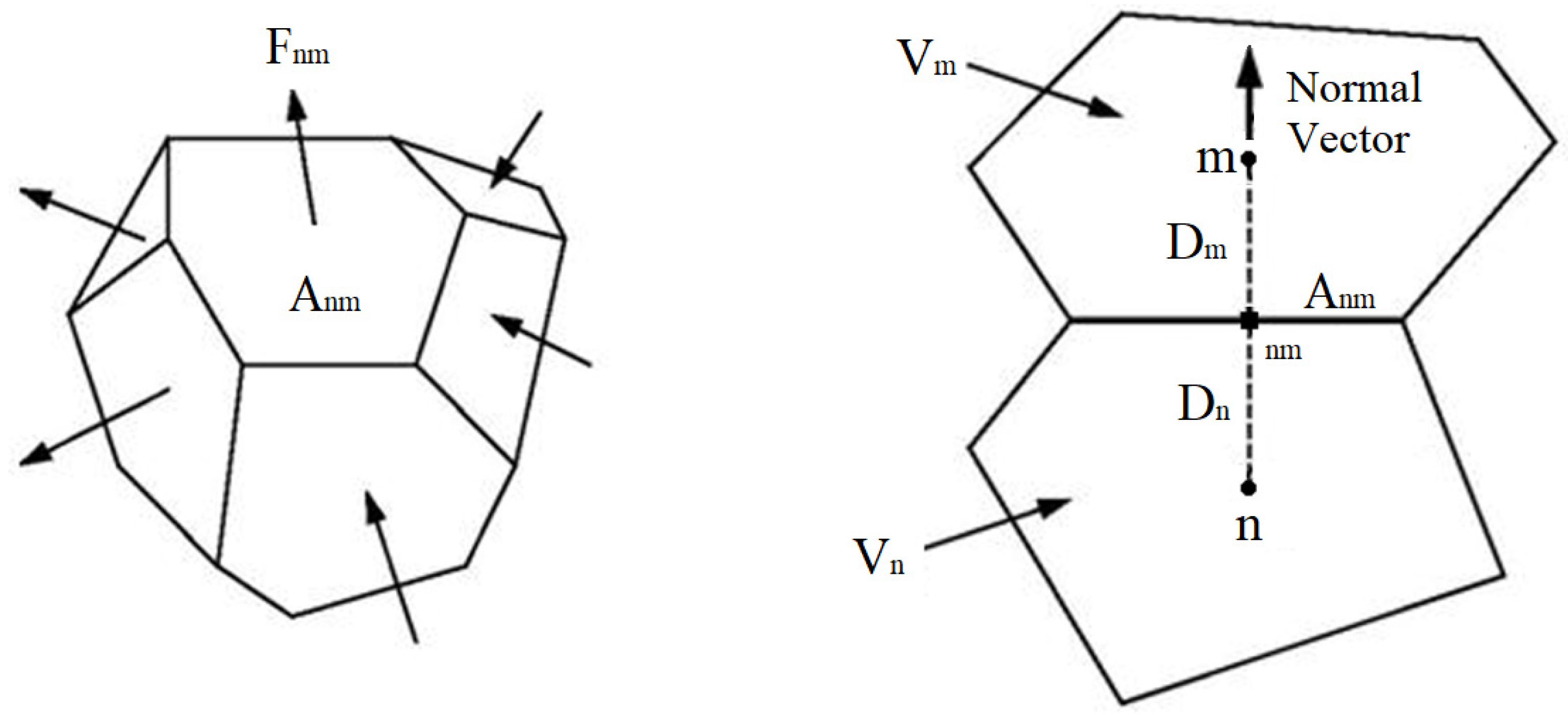
3.1. Numerical Discretization of Space and Time

The IFD was used to discretize the space domain for PDE introduced in Section 2 and can be adopted into both structured and unstructured grids.

3.1.1. Discretization of Mass and Energy Balance Equations

The principle behind the IFD is to integrate the PDE with respect to the volume of the gridblock:

$${\displaystyle \frac{d}{dt}}{{\displaystyle \int }}_{V_n}{M}^{k}d{V}_n=-{{\displaystyle \int }}_{V_n}\nabla ·\overrightarrow{F^k}d{V}_n+{{\displaystyle \int }}_{V_n}{q}^{k}d{V}_n$$

(22)

in which $V_n$ represents the volume of gridblock n. Due to the divergence theorem, the integration of the flux term turns into a net flux term of surface integration:

$${\displaystyle \frac{d}{dt}}{{\displaystyle \int }}_{V_n}{M}^{k}d{V}_n=-{{\displaystyle \int }}_{{\Gamma }_n}\overrightarrow{F^k}·\widehat{n}d{\Gamma }_n+{{\displaystyle \int }}_{V_n}{q}^{k}d{V}_n$$

(23)

in which ${\Gamma }_n$ is the surface area of the current gridblock and $\widehat{n}$ is the normal vector pointing outwards the internal volume. The integration can be replaced by a summation when the reservoir domain is discretized into a set of gridblocks or elements:

$${\displaystyle \frac{d}{dt}}\left(M_n^k{V}_{n,0}\left(1-{\epsilon }_{v,n}\right)\right)=-{\displaystyle {\displaystyle \sum }_m}{A}_{nm,0}\left(1-{\epsilon }_{A,nm}\right)F_{nm}^k+q_n^k{V}_{n,0}\left(1-{\epsilon }_{v,n}\right)$$

(24)

in which volumetric strain, ${\epsilon }_{v,n}$, and areal strain, ${\epsilon }_{A,nm}$, are secondary parameters calculated by stresses, in order to account for the geomechanical impact on the dimensions of the gridblocks. In Equation (24), $V_{n,0}$ is the initial gridblock volume and $A_{nm,0}$ is the interface area between two connected gridblocks n and m; $F_{nm}^{\kappa }$ is the mass flux of component $\kappa$ between gridblock n and gridblock m. The illustration of two connected gridblocks and net flux of a single gridblock is shown in Figure 1. The flux between gridblock n and gridblock m can be written by the ‘discretized’ form of Darcy’s law:

$$A_{nm}\left(1-{\epsilon }_{A,nm}\right)F_{nm}^k={{\displaystyle \sum }}_{\beta }-k_{nm}{\left({\displaystyle \frac{k_{r\beta }{\rho }_{\beta }{X}_{\beta }^k}{{\mu }_{\beta }}}\right)}_{nm}\left({\displaystyle \frac{P_n+P_{c\beta ,n}-P_m-P_{c\beta ,m}}{D_{n,0}\left(1-{\epsilon }_{D,n}\right)+D_{m,0}\left(1-{\epsilon }_{D, m}\right)}}-{\rho }_{\beta ,nm}{g}_{nm}\right)A_{nm,0}(1-{\epsilon }_{A,nm})$$

(25)

in which the subscript nm of term ${\left({\displaystyle \frac{k_{r\beta }{\rho }_{\beta }{X}_{\beta }^k}{{\mu }_{\beta }}}\right)}_{nm}$ implies that relative permeability, density, viscosity, and mass fraction should be evaluated at the interface through a certain weighting scheme, such as upstream weighting. The normal strain ${\epsilon }_{D,n}$ and ${\epsilon }_{D,m}$ are also secondary variables computed by a linear elastic relation.

For the energy balance equation, the heat flow term is similarly expressed as follows:

$$\begin{array}{l}{A}_{nm}\left(1-{\epsilon }_{A,nm}\right)F_{nm}^{NK+1}\\ =-{\lambda }_{nm}\left(T_n-T_m\right)A_{nm,0}\left(1-{\epsilon }_{A,nm}\right)\\ +{\displaystyle {\displaystyle \sum }_{\beta }}-k_{nm}{\left({\displaystyle \frac{k_{r\beta }{\rho }_{\beta }{X}_{\beta }^k}{{\mu }_{\beta }}}{h}_{\beta }\right)}_{nm}\left({\displaystyle \frac{P_n+P_{c\beta ,n}-P_m-P_{c\beta ,m}}{D_{n,0}\left(1-{\epsilon }_{D,n}\right)+D_{m,0}\left(1-{\epsilon }_{D, m}\right)}}-{\rho }_{\beta ,nm}{g}_{nm}\right)A_{nm,0}(1-{\epsilon }_{A,nm})\end{array}$$

(26)

3.1.2. Discretization of Momentum Balance Equation

The discretization of the momentum balance equation is also based on the IFD approach [25]. The form of equation is similar to that of Equation (1), without sink/source or accumulation terms:

$${{\displaystyle \int }}_{{\Gamma }_n}\overrightarrow{F^{NK+2}}·\widehat{n}d{\Gamma }_n=0$$

(27)

The flux term can be expressed from Equation (15) as follows:

$$\overrightarrow{F^{NK+2}}={\mathsf{\Psi }}_{\mathsf{\tau },\mathrm{nm}}={\displaystyle \frac{3\left(1-\nu \right)}{1+\nu }}\nabla {\tau }_m+\overrightarrow{F_b}-{\displaystyle \frac{2\left(1-2\nu \right)}{1+\nu }}\nabla \left[h\left(\overline{P},\overline{T}\right)\right]$$

(28)

Equation (28) is called momentum flux, which is comparable with Equation (4) or Equation (7). There are two methods of computing such type of ‘flux’ between two connected gridblocks shown in Figure 1. One method is similar to Equations (25) and (26):

$$\begin{array}{c}{\displaystyle {\displaystyle \sum }_m}{A}_{nm,0}\left(1-{\epsilon }_{A,nm}\right)\{{\left({\displaystyle \frac{3\left(1-\nu \right)}{1+\nu }}\right)}_{nm}{\displaystyle \frac{{\tau }_n-{\mathsf{\tau }}_m}{D_{n,0}\left(1-{\epsilon }_{D,n}\right)+D_{m,0}\left(1-{\epsilon }_{D, m}\right)}}+F_{b,nm}\\ -{\left({\displaystyle \frac{2\left(1-2\nu \right)}{1+\nu }}\right)}_{nm}{\displaystyle \frac{h{\left(\overline{P},\overline{T}\right)}_n-h{\left(\overline{P},\overline{T}\right)}_m}{D_{n,0}\left(1-{\epsilon }_{D,n}\right)+D_{m,0}\left(1-{\epsilon }_{D, m}\right)}} \}=0\end{array}$$

(29)

This approach is adopted from [12,24,47]. However, it has the drawback that the interface quantities ${\left({\displaystyle \frac{3\left(1-\nu \right)}{1+\nu }}\right)}_{nm}$ and ${\left({\displaystyle \frac{2\left(1-2\nu \right)}{1+\nu }}\right)}_{nm}$ may not be properly evaluated if mechanical properties are heterogeneous—for instance, if Poisson’s ratio differs at element n and element m. In another approach of flux computation, interface stress is calculated first by assuming that the flux from gridblock n to gridblock m is equal to that from n to interface and to that from interface to m: ${\Psi }_{\tau ,n-nm}={\Psi }_{\tau ,nm-m}={\Psi }_{\tau ,nm}$. The momentum flux from n to interface is expressed as follows:

$${\Psi }_{\tau ,\mathrm{n}-\mathrm{nm}}={\displaystyle \frac{3\left(1-{\nu }_{\mathrm{n}}\right)}{1+{\nu }_{\mathrm{n}}}}{\displaystyle \frac{{\tau }_{m,\mathrm{n}}-{\tau }_{m,nm}}{D_{\mathrm{n}}}}+\overrightarrow{F_{b,n}}-{\displaystyle \frac{2\left(1-2{\nu }_{\mathrm{n}}\right)}{1+{\nu }_{\mathrm{n}}}}{\displaystyle \frac{h{\left(P,T\right)}_{\mathrm{n}}-h{\left(\overline{P},\overline{T}\right)}_{n,nm}}{D_{\mathrm{n}}}}$$

(30)

where the thermal and pore pressure term is as follows:

$$\mathrm{h}{\left(\overline{P},\overline{T}\right)}_{\mathrm{n},\mathrm{nm}}={{\displaystyle \sum }}_j{\alpha }_{j,n}{P}_{nm}+3{\beta }_n{K}_n{\omega }_{j,n}\left(T_{nm}-T_{ref}\right)$$

(31)

Similarly, the flux from interface to element m is expressed as follows:

$${\Psi }_{\tau ,\mathrm{nm}-\mathrm{m}}={\displaystyle \frac{3\left(1-{\nu }_{\mathrm{m}}\right)}{1+{\nu }_{\mathrm{m}}}}{\displaystyle \frac{{\tau }_{m,\mathrm{nm}}-{\tau }_m}{D_{\mathrm{m}}}}+\overrightarrow{F_{b,m}}-{\displaystyle \frac{2\left(1-2{\nu }_{\mathrm{m}}\right)}{1+{\nu }_{\mathrm{m}}}}{\displaystyle \frac{h{\left(\overline{P},\overline{T}\right)}_{m,nm}-h{\left(\overline{P},\overline{T}\right)}_{\mathrm{m}}}{D_{\mathrm{m}}}}$$

(32)

Equations (30) and (32) are combined to solve interface mean stress, ${\tau }_{m,nm}$, and flux, ${\Psi }_{\tau ,nm}$:

$${\Psi }_{\tau ,nm}={\displaystyle \frac{\left\{\begin{array}{c}{\tau }_{m,\mathrm{n}}-{\tau }_{m,\mathrm{n}}+{\displaystyle \frac{D_{\mathrm{n}}\left(1+{\nu }_{\mathrm{n}}\right)}{3\left(1-{\nu }_{\mathrm{n}}\right)}}\overrightarrow{F_{b,n}}\widehat{·n}+{\displaystyle \frac{{\mathrm{D}}_{\mathrm{m}}\left(1+{\nu }_{\mathrm{m}}\right)}{3\left(1-{\nu }_{\mathrm{m}}\right)}}\overrightarrow{F_{b,m}}\widehat{·n}\\ -{\displaystyle \frac{2\left(1-2{\nu }_{\mathrm{n}}\right)}{3\left(1-\mathrm{n}\right)}}\left(h{\left(\overline{P},\overline{T}\right)}_{\mathrm{n}}-h{\left(\overline{P},\overline{T}\right)}_{\mathrm{n},\mathrm{nm}}\right)-{\displaystyle \frac{2\left(1-2{\nu }_{\mathrm{m}}\right)}{3\left(1-{\nu }_{\mathrm{m}}\right)}}\left(h{\left(\overline{P},\overline{T}\right)}_{\mathrm{m},\mathrm{nm}}-h{\left(\overline{P},\overline{T}\right)}_{\mathrm{m}}\right)\end{array}\right\}}{{\displaystyle \frac{{\mathrm{D}}_{\mathrm{n}}\left(1+{\nu }_{\mathrm{n}}\right)}{3\left(1-{\nu }_{\mathrm{n}}\right)}}+{\displaystyle \frac{{\mathrm{D}}_{\mathrm{m}}\left(1+{\nu }_{\mathrm{m}}\right)}{3\left(1-{\nu }_{\mathrm{m}}\right)}}}}$$

(33)

$${\tau }_{m,\mathrm{nm}}={\tau }_{m,\mathrm{n}}-{\displaystyle \frac{{\mathrm{D}}_{\mathrm{n}}\left(1+{\nu }_{\mathrm{n}}\right)}{3\left(1-{\nu }_{\mathrm{n}}\right)}}\left({\Psi }_{\tau ,\mathrm{nm}}-\overrightarrow{F_{b,n}}+{\displaystyle \frac{2\left(1-2{\nu }_{\mathrm{n}}\right)}{1+{\nu }_{\mathrm{n}}}}{\displaystyle \frac{h{\left(\overline{P},\overline{T}\right)}_{\mathrm{n}}-h{\left(\overline{P},\overline{T}\right)}_{\mathrm{n},\mathrm{nm}}}{{\mathrm{D}}_{\mathrm{n}}}}\right)$$

(34)

Pressure and temperature at the interface in Equation (31) are calculated using mass flux conservation and harmonic averaging, respectively. $P_{nm}$, ${\tau }_{m,\mathrm{nm}}$, and $T_{nm}$ are updated at each Newton’s iteration and then Equation (27) can be rewritten as a summation:

$${\displaystyle {\displaystyle \sum }_m}{A}_{nm,0}\left(1-{\epsilon }_{A,nm}\right){\Psi }_{\tau ,nm}=0$$

(35)

This approach of flux computation was adopted from [25,32].

In [25], stress tensor components were updated at the end of each time step using Equations (16)–(21) with the solved mean stress. Take normal stress in x direction as an example: Equation (16) needed to be discretized using the IFD method with the same approach of flux computation performed by Equations (30) and (34) and flux of momentum in x direction can be obtained:

$${\Psi }_{xx,nm}={\displaystyle \frac{\left\{\begin{array}{c}{\tau }_{xx,\mathrm{n}}-{\tau }_{xx,\mathrm{m}}\\ +2D_{\mathrm{n}}{F}_{b,x,\mathrm{n}}+2D_{\mathrm{m}}{F}_{b,x,m}-{\displaystyle \frac{3{\nu }_{\mathrm{n}}}{1+{\nu }_{\mathrm{n}}}}\left({\tau }_{m,\mathrm{n}}-{\tau }_{m,nm}\right)-{\displaystyle \frac{3{\nu }_{\mathrm{m}}}{1+{\nu }_{\mathrm{m}}}}\left({\tau }_{m,\mathrm{m}}\right)\\ +{\displaystyle \frac{3\widehat{n}·\widehat{i}}{1+{\nu }_{\mathrm{n}}}}\left({\tau }_{m,\mathrm{n}}-{\tau }_{m,nm}\right)+{\displaystyle \frac{3\widehat{n}·\widehat{i}}{1+{\nu }_{\mathrm{m}}}}\left({\tau }_{m,nm}-{\tau }_{m,\mathrm{m}}\right)\\ +{\displaystyle \frac{2{\nu }_{\mathrm{n}}-1}{1-{\nu }_{\mathrm{n}}}}\left(1+\widehat{n}·\widehat{i}\right)\left(h{\left(\overline{P},\overline{T}\right)}_{\mathrm{n}}-h{\left(\overline{P},\overline{T}\right)}_{\mathrm{n},nm}\right)\\ +{\displaystyle \frac{2{\nu }_{\mathrm{m}}-1}{1-{\nu }_{\mathrm{m}}}}\left(1+\widehat{n}·\widehat{i}\right)\left(h{\left(\overline{P},\overline{T}\right)}_{\mathrm{m},nm}-h{\left(\overline{P},\overline{T}\right)}_{\mathrm{m}}\right)\end{array}\right\}}{\frac{D_{\mathrm{n}}\left(1+{\nu }_{\mathrm{n}}\right)}{3\left(1-{\nu }_{\mathrm{n}}\right)}+\frac{D_{\mathrm{m}}\left(1+{\nu }_{\mathrm{m}}\right)}{3\left(1-{\nu }_{\mathrm{m}}\right)}}}$$

(36)

At the end of each time step, mean stresses are solved by Newton’s method along with pressure, saturation, and temperature, and with the update of interface quantities, the normal stresses can be solved by Equation (36). Ref. [32] extended this methodology to solve the governing Equations (16)–(21) in Newton’s iteration, adding normal stresses in x and y directions and three shear stresses into the list of primary variables. The coupled model becomes a fully coupled one with the capability of solving full stress tensor components. This extension aims mainly at the embedded discrete fracture, which will be explained later in this paper.

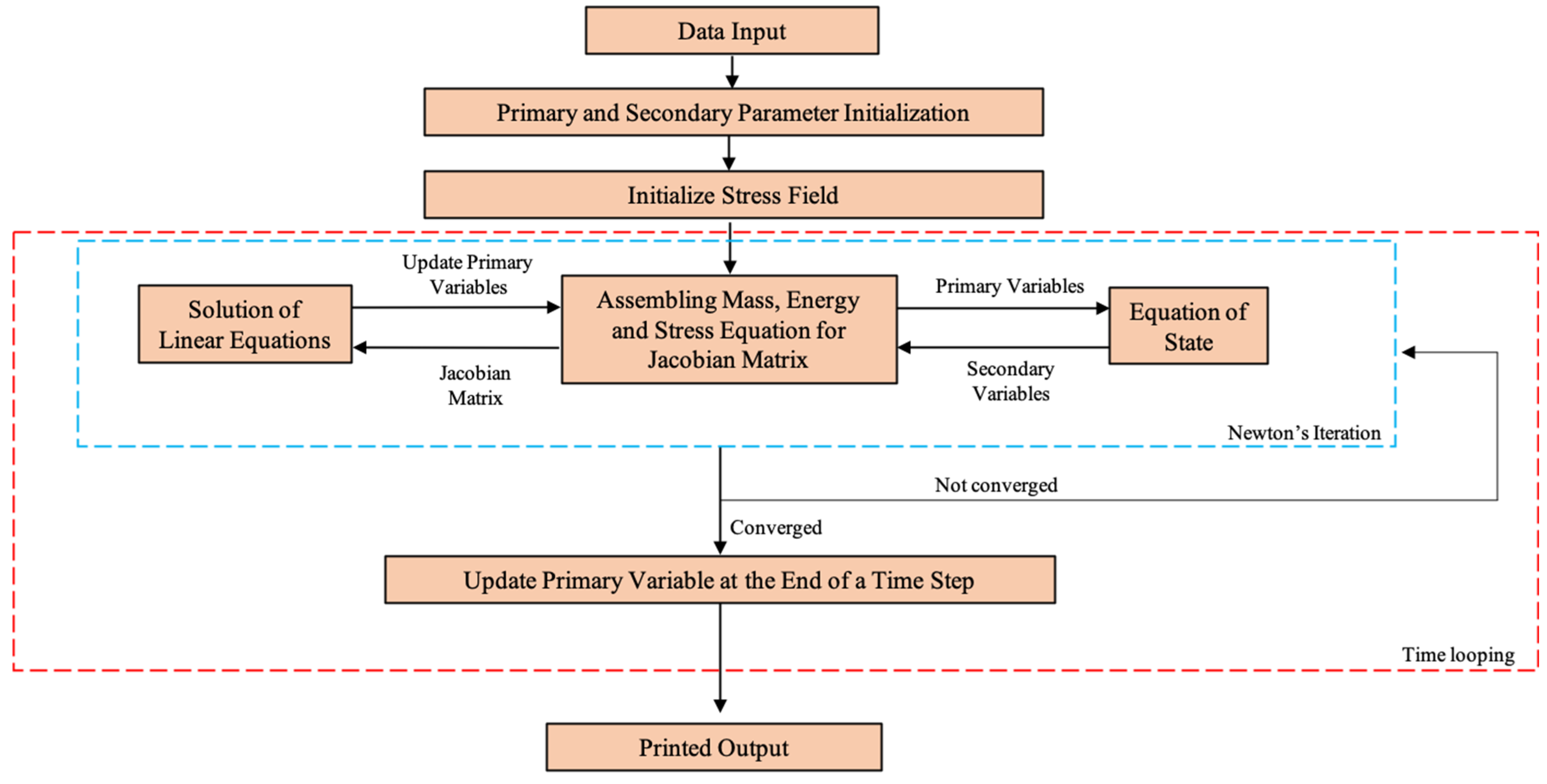
3.2. Numerical Solution Approach

The dependency of secondary variables or parameters, such as density, internal energy, enthalpy, porosity, permeability, viscosity, and relative permeability, on primary variables (pressure, saturation, temperature, and stresses) increases the non-linearity of the governing PDEs. Solutions of such a highly non-linear system are usually achieved by Newton’s method in which iterations are conducted to seek a convergence for a time step. In this section, this Newton iteration method will be briefly illustrated.

Newton’s method provides an approach to iteratively solve a system of nonlinear equations. Each gridblock in the reservoir domain has a number of residual equations that equal to the number of governing equations:

$$R_n^{\kappa ,i+1}={\left(M_n^{\kappa }\left(1-{\epsilon }_{v,n}\right)\right)}^{i+1}-{\left(M_n^{\kappa }\left(1-{\epsilon }_{v,n}\right)\right)}^i-\Delta t{\displaystyle {\displaystyle \sum }_m}{\left({\displaystyle \frac{A_{nm,0}}{V_{n,0}}}\left(1-{\epsilon }_{A,nm}\right)F_{nm}^{\kappa }\right)}^{i+1}-\Delta t{\left(q_n^{\kappa }\left(1-{\epsilon }_{v,n}\right)\right)}^{i+1}$$

(37)

where $\kappa$ represents the index of governing equation and $\mathrm{n}$ is the index of gridblock, $i+1$ stands for quantities that are evaluated at the $i+1$ (new) time step level, and $i$ stands for quantities calculated at the previous time step level. The objective of Newton’s method is to reduce the residual in Equation (37) to zero. When residual equations are treated to be a function of all the primary variables of gridblock n and its direct neighboring gridblocks m’s, the residual equation can be expressed by a first-order Taylor’s expansion,

$$R_n^{\kappa ,p+1}\left(x_{l,p+1}\right)=R_n^{\kappa ,p+1}\left(x_{l,p}\right)+{\displaystyle {\displaystyle \sum }_l}{\displaystyle \frac{\partial R_n^{k,p+1}}{\partial x_l}}{│}_p\left(x_{l,p+1}-x_{l,p}\right)$$

(38)

Newton’s method of multi-variables can be comparable to the Newton–Raphson’s approach for a single variable, making residual in Equation (38) approach zero:

$$-{\displaystyle {\displaystyle \sum }_l}{\displaystyle \frac{\partial R_n^{k,p+1}}{\partial x_l}}{│}_p\left(x_{l,p+1}-x_{l,p}\right)=R_n^{\kappa ,p+1}\left(x_{l,p}\right)$$

(39)

Equation (39) states that the primary variable vector at iteration level $p+1$ can be solved by computing all residuals at iteration level $p$ $\left(R_n^{\kappa ,p+1}\left(x_{l,p}\right)\right)$ and all residual derivative or Jacobian terms at iteration level $p$ (${\displaystyle \frac{\partial R_n^{k,p+1}}{\partial x_l}}{│}_p$). The left-hand-side derivatives establish a linear system, called the Jacobian matrix, and the solution of the linear system marks the completion of one Newton’s iterations.

The program structures of the simulators in [12,25,32] are almost the same as shown in Figure 2. The input files are read for all input data, including mesh/grid data and the initial states of pressure, saturation, and temperature. Then the stress field will be initialized by the input boundary stress conditions. Then the time-stepping loop is started, in which Newton’s iteration is performed to seek convergence. Residual equations are computed by looping around all elements and all connections for accumulation and flow terms. Derivatives are calculated to assemble the Jacobian matrix, which is solved by an appropriate linear solver. In [25], mean stress is treated as a primary variable and there will be an additional step of solving for all other stress tensor components out of the Newton’s iteration loop and within the time-stepping loop. In comparison, all stress tensor components in [32] are solved implicitly in Newton’s iteration so that the additional step is not necessary.

Our simulator is massively parallelized, with domain partitioning using the METIS and ParMETIS packages [48,49]. Each processor computes Jacobian matrix elements for its own grid blocks, and exchange of information between processors uses the MPI (Message Passing Interface) and allows calculation of Jacobian matrix elements associated with inter-block connections across domain partition boundaries. The Jacobian matrix is solved in parallel using an iterative linear solver from the PETSc [50] package.

4. Model Validation

The geomechanics module of the coupled model introduced in this paper is based on IFD discretization, which is a new methodology that has not been widely adopted. It is necessary to validate the coupled model using existing simulators or analytical solutions. In this section, validation cases are provided for the coupled model to prove its accuracy and capability.

4.1. Validation Using an Existing Simulation Case

Ref. [25] validated their model using two analytical models and two existing simulation cases. One of the existing simulation cases will be reviewed in this paper. Ref. [51] modeled the process of CO₂ injection into a depleted gas reservoir for geological sequestration in In Salah, Algeria. The surface uplift was modeled by the coupled THM model TOUGH2- FLAC. In the TOUGH2-FLAC coupled simulator [5], TOUGH2 [43] and FLAC [52] are coupled in a sequential manner with data exchanges between them. FLAC solves the geomechanical equations and transmits effective stress and strain to TOUGH2; TOUGH2 solves the flow equations and transmits updated porosity back to FLAC. The level of this coupling, such as during the Jacobian calculation, the end of each Newton iteration, or at each time step, is variable. On the other hand, our model solves the flow and geomechanical equations simultaneously. Ref. [25] reconstructed the model on a finer mesh grid and ran the simulation case with their in-house simulator for the coupled THM model.

The modeled domain has a dimension of 10 km in the x-direction, 10 km in the y-direction, and 4 km in the z-direction. There are four layers from the surface down to the bottom: shallow overburden, caprock, injection reservoir, and base. The input parameters of all the four layers are shown in

Table 1. Input parameters for validation cases [25].

Parameters	Shallow Overburden (0–900 m)	Caprock (900–1800 m)	Injection Zone (1800–1820 m)	Base (>1820 m)
Young’s modulus (GPa)	1.5	20.0	6.0	20.0
Poisson’s ratio	0.2	0.15	0.2	0.15
Biot’s coefficient	1.0	1.0	1.0	1.0
Porosity	0.1	0.01	0.17	0.01
Permeability (m2)	1.0 × 10−17	1.0 × 10−19	0.875 × 10−14	1.0 × 10−21
Residual CO2 saturation	0.05	0.05	0.05	0.05
Residual liquid saturation	0.3	0.3	0.3	0.3
CO2 injection rate (kg/s)			9.734
Initial injection well pressure (MPa)			18.5
Injection time (years)			3

. The reservoir domain is at hydrostatic equilibrium and water is the only reservoir fluid. Hydrostatic initial condition is generated and input into the simulator for stress tensor component initialization. It has been assumed that no shear stresses exist initially in the stress field and the normal stresses components only vary in the z-direction. Therefore, Equation (8) is reduced to the following:

$${\displaystyle \frac{\partial {\mathsf{\tau }}_{\mathrm{zz}}}{\partial z}}+F_{b,z}=0$$

(40)

and Equations (16) and (17) and are reduced to the following:

$${\displaystyle \frac{{\partial }^2}{\partial z^2}}\left({\tau }_{xx}-h\left(\overline{P},\overline{T}\right)-{\displaystyle \frac{3\nu }{1+\nu }}\left({\tau }_m-h\left(\overline{P},\overline{T}\right)\right)\right)=0$$

(41)

$${\displaystyle \frac{{\partial }^2}{\partial z^2}}\left({\tau }_{yy}-h\left(\overline{P},\overline{T}\right)-{\displaystyle \frac{3\nu }{1+\nu }}\left({\tau }_m-h\left(\overline{P},\overline{T}\right)\right)\right)=0$$

(42)

It can be seen that Equations (41) and (42) are capable of initializing the stress field if the stress state at the boundary is known. This is the approach of stress initialization for the model introduced in Section 3.2. The reservoir has a constant stress at each boundary and pore pressures are assumed to be equal to boundary gridblocks’ value for geomechanical computation. The gridblock size in the z-direction can be calculated by the following:

$$\mathsf{\Delta }{z}_k=\mathsf{\Delta }{z}_{k,i}{\displaystyle \frac{1-{\epsilon }_{zz}}{1-{\epsilon }_{zz,i}}}$$

(43)

in which subscript i represents the initial value and the surface displacement is calculated by the combining effect of vertical displacement of all gridblocks in the z-direction.

The model in [25] is of dimension 5 km × 5 km × 4 km with a grid dimension of 50 × 50 × 60. Simulation results of pressure changes and vertical displacements are shown in Figure 3. The good match between two models validates the accuracy and capability of the coupled THM model of this paper.

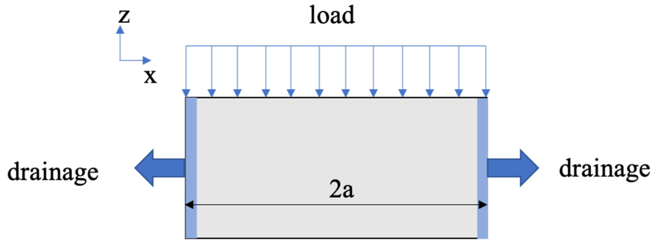
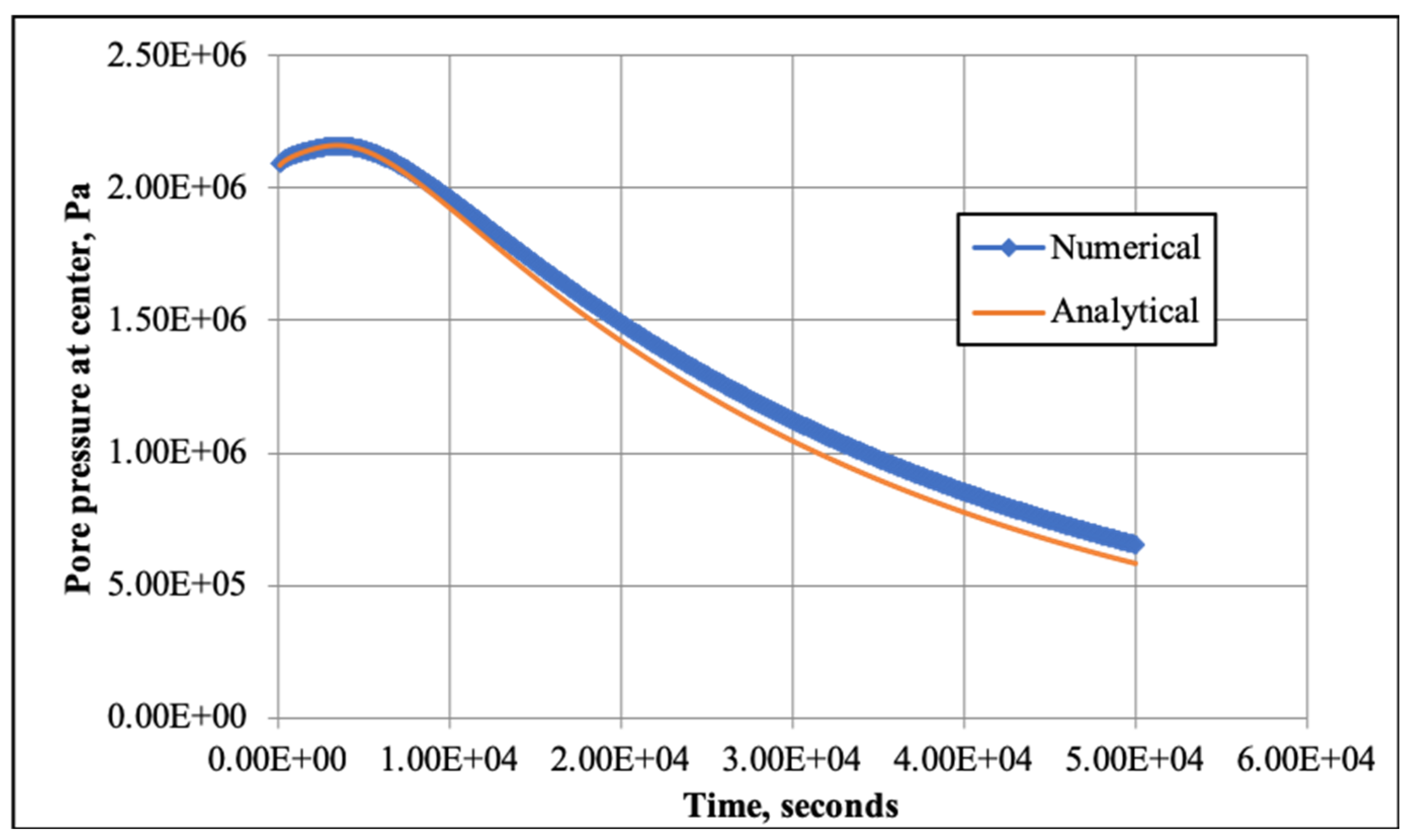
4.2. Validation Using an Analytical Solution

Ref. [32] validated their coupled THM model where full stress tensor components are solved implicitly, using the analytical solution ‘Mandel’s problem’ [53]. Mandel’s problem states that when a rectangular sample is subject to a constant load on top and the lateral boundaries are allowed to drain fluid, the pore pressure at the center of the sample will increase before being reduced by drainage. This is because the stress variation propagates faster than the pressure and the stress increases in the center of the material before the pore pressure is dissipated. The schematic of the model is shown in Figure 4.

Ref. [54] derived an analytical solution to Mandel’s problem:

$${\displaystyle \frac{p}{p_0}}={\displaystyle \frac{{\sum }_{j=1}^{\infty }\frac{\sin \left({\xi }_j\right)\left[\cos \left(\frac{{\xi }_{j}x}{a}\right)-\cos \left({\xi }_j\right)\right]}{{\xi }_j-\sin \left({\xi }_j\right)\cos \left({\xi }_j\right)}\exp \left(\frac{-{\xi }_j^2{c}_{v}t}{a^2}\right)}{{\sum }_{j=1}^{\infty }\frac{\sin \left({\xi }_j\right)\left[\cos \left(\frac{{\xi }_{j}x}{a}\right)-\cos \left({\xi }_j\right)\right]}{{\xi }_j-\sin \left({\xi }_j\right)\cos \left({\xi }_j\right)}}}$$

(44)

where ${\xi }_j$ represents the root of $\tan \left(\xi \right)=\eta \xi$, $x$ is the distance away from the center of the sample, and $t$ is the time after the start of drainage. Additionally, $\eta ={\displaystyle \frac{3\left(1-\nu \right)}{2\left(1-2\nu \right)}}{\displaystyle \frac{K{C}_f+\alpha }{\alpha }}$ and $c_v={\displaystyle \frac{k}{\mu }}{\displaystyle \frac{1}{\frac{\varphi \left(1+\nu \right)}{3K\left(1-\nu \right)}+C_f\varphi }}$, where $K$ is bulk modulus, $\nu$ is the Poison’s ratio, $C_f$ is the fluid compressibility, $\alpha$ is Biot’s coefficient, $k$ is the sample permeability, $\mu$ is fluid viscosity, and $\varphi$ is porosity. The sample dimension is set to 1001 m × 1001 m × 10 m, with 51 × 51 × 1 gridblocks. The top gridblocks are considered to be a constant stress flux boundary. The simulation was conducted in two parts: (1) simulation of the pore pressure increase due to the load, and (2) simulation of the drainage process. The pore pressure at the center was observed and compared with the analytical solution, as shown in Figure 5. The input parameters are shown in

Table 2. Input parameters for Mandel’s problem.

Parameters	Value	Unit
Matrix permeability	1 × 10−13	m2
Initial pore pressure	1× 105	Pa
Initial sample temperature	60	°C
Production (constant pressure)	1× 105	Pa
Rock/fracture porosity	0.094	Unitless
Production well index	1.7 × 10−9	m3
Rock expansion coefficient	4 × 10−6	1/°C
Poisson’s ratio	0.25	Unitless
Young’s modulus	5	GPa
Biot’s coefficient	1	Unitless
Water viscosity (@ 60 °C, analytical)	0.00046	Pa-s
Water compressibility (analytical)	4.04 × 10−10	1/Pa
Water density (analytical)	983	kg/m3

.

5. Model Application into Geothermal Reservoir Simulation

The coupled THM model is essential for geothermal reservoir simulation, as has been explained. The methodology introduced in this paper can be applied to geothermal reservoir simulation for a wide scope of scenarios, especially fractured geothermal reservoirs. Geothermal energy production from an EGS reservoir is highly dependent on artificial hydraulic fractures, which are sensitive to geomechanics, especially thermal stresses. Rock volume is subject to significant shrinkage when cold water is flowing through the fractures. As a result, fracture apertures will be expanded, and permeability will be enhanced. In this section, our coupled THM model was applied to three different simulation cases: (1) a fractured geothermal reservoir modeled by the classical double-porosity approach, (2) a geothermal reservoir with hydraulic fractures modeled by EDFM, and (3) tracer transport in a geothermal reservoir with hydraulic fractures modeled by EDFM. In the first two cases, thermal stress and production compaction impact will be observed for water injection and heat production. In the last case, the tracer transport case will be applied into a real geothermal engineering project.

5.1. Coupled THM Model with Double-Porosity Approach

Ref. [12] developed a semi-analytical solution to calculate the fracture aperture expansion due to the cold water injection. It has been assumed by [12] that when cold water reaches the fracture, the heat convection between fracture and matrix is a slow process compared to heat conduction due to the low permeability and stiff nature of the rock matrix. Therefore, the governing equation can be simplified by reducing the fluid flow part and considering only the heat conduction effect. The 3D matrix block can be modeled by a spherical body by analogy to the double porosity developed by [33]. The spherical body has a radius called the characteristic length, $L_c$, which can be calculated by the matrix block dimensions:

$${\displaystyle \frac{4}{3}}\pi L_c^3=L_x{L}_y{L}_z$$

(45)

Then, the governing mechanical Equation (12) can be transformed into a 1D system:

$${\displaystyle \frac{\partial }{\partial \mathrm{r}}}\left[{\displaystyle \frac{1}{r^2}}{\displaystyle \frac{\partial }{\partial r}}\left(r^2{u}_r\right)\right]={\displaystyle \frac{1+\nu }{1-\nu }}\beta {\displaystyle \frac{\partial }{\partial r}}\left(T_m-T_{m0}\right)$$

(46)

with an intuitive boundary condition that the displacement at the center of body equals to zero:

$${\mathrm{u}}_{\mathrm{r}}\left(r=0,t\right)=0$$

(47)

Equation (46) can be solved by integration:

$$u_r={\displaystyle \frac{1}{r^2}}{\displaystyle \frac{1+\nu }{1-\nu }}\beta \int \left(T_m-T_{m0}\right)r^{2}dr+Cr$$

(48)

And constant C should be solved by the other boundary condition: stress condition at $r=L_c$. This stress condition can be derived by the force equilibrium: the force generated due to the fracture stiffness is equilibrated to the force induced by the displacement of rock matrix, combining the pore pressure change in fractures:

$$\Delta {\sigma }_{rr}{│}_{r=L_c}=-k_{f}u{│}_{r=L_c}-\left(P_f-P_{f0}\right)$$

(49)

in which $k_f$ is the fracture stiffness and

$$\Delta {\sigma }_{rr}={\displaystyle \frac{E_m}{\left(1+\nu \right)\left(1-2\nu \right)}}\left[\left(1-\nu \right){\displaystyle \frac{\partial u_r}{\partial r}}+2\nu {\displaystyle \frac{u_r}{r}}-\left(1+\nu \right)\beta \left(T_m-T_{m,0}\right)\right]$$

(50)

The constant $\mathrm{C}$ can be solved by combining Equations (48)–(50):

$$C={\displaystyle \frac{-\left(P_f-P_{f0}\right)+\frac{1}{3}\beta \left({\overline{T}}_m-T_{m0}\right)\frac{2E_m}{1-2\nu }-\frac{1}{3}{k}_f\frac{1+\nu }{1-\nu }\left({\overline{T}}_m-T_{m0}\right)L_c}{\frac{E_m}{1-2\nu }+k_f{L}_C}}$$

(51)

in which ${\overline{T}}_m$ is the average temperature of matrix block that replaces the integration:

$${\displaystyle \frac{1}{{\mathrm{r}}^2}}{{\displaystyle \int }}_0^{L_C}\left(T_m-T_{m0}\right)r^{2}dr={\displaystyle \frac{1}{3}}{L}_C\left({\overline{T}}_m-T_{m0}\right)$$

(52)

Plug Equation (51) into Equation (48) and the fracture aperture change can be obtained:

$$\Delta b_i=-2u_i\left(L_C\right)=2{\displaystyle \frac{\left(P_f-P_{f0}\right)-\beta \left({\overline{T}}_m-T_{m0}\right)\frac{E_m}{1-2\nu }}{\frac{E_m}{1-2\nu }+k_f{L}_C}}·L_C$$

(53)

Ref. [12] validated this correlation using a commercial multi-physics simulator, COMSOL, by setting up a model where rock matrix displacement (or deformation) is computed due to the lower fracture temperature. When fracture stiffness is not constant, but a function of stress, the constant $C$ can be solved by a nonlinear iterative method. Fracture aperture will then be solved after $C$ is obtained.

This methodology is then applied to a fractured geothermal reservoir, shown in Figure 6. The parameters for the model are obtained from a geothermal field in Australia. The reservoir dimension is 762 m × 762 m × 152 m. The injected zone has an initial pore pressure of 7.0 MPa and temperature of 220 °C. The system is overburdened by an impermeable caprock and the vertical stress at the top is 90 MPa; the two horizontal stresses are 140 MPa and 110 MPa. Lateral boundaries are all fixed to be a zero normal displacement boundary (uniaxial strain). Cold water with a temperature of 80 °C is injected with a constant rate of 12 kg/s into the reservoir for 7 years and hot water is produced at a bottom hole pressure of 5.0 MPa. Initial fracture aperture is back-calculated from the initial fracture permeability using the cubic law [55]:

$${\mathrm{k}}_{\mathrm{fi}0}={\displaystyle \frac{C_i{\left(b_{i0}\right)}^3}{12{\mathrm{L}}_{\mathrm{i}}}}$$

(54)

During the simulation, when fracture aperture varies according to the temperature change, fracture permeability variation is determined by the following equation:

$${\mathrm{k}}_{\mathrm{fi}}=k_{fi0}{\displaystyle \frac{{\left(b_{i0}+\mathsf{\Delta }{b}_i\right)}^3}{{\left(b_{i0}\right)}^3}}$$

(55)

Matrix porosity can be calculated by the following correlation proposed by [19]:

$$\varphi ={\varphi }_{\mathrm{r}}+\left({\varphi }_0-{\varphi }_r\right)\exp \left(-a{{\sigma }_m}^{\prime }\right)$$

(56)

where ${\varphi }_{\mathrm{r}}$ is the residual matrix porosity, ${\varphi }_0$ is the matrix porosity at zero-stress state, and ${{\sigma }_m}^{\prime }$ is effective stress applied on the matrix gridblock. Based on matrix porosity, matrix permeability can be calculated by the Carman–Kozeny equation [56]:

$${\mathrm{k}}_{\mathrm{m}}=k_{m0}{\left({\displaystyle \frac{1-{\varphi }_0}{1-\varphi }}\right)}^3{\left({\displaystyle \frac{\varphi }{{\varphi }_0}}\right)}^3$$

(57)

Input parameters for this geothermal reservoir model are shown in

Table 3. Input parameters for the geothermal reservoir model using the double-porosity approach and fracture aperture correlation.

Properties	Values	Units
Initial permeability of the fracture continuum	Kf = 1.0 × 10−11	m2
Initial permeability of the matrix continuum	Kmx = 1.0 × 10−15	m2
Porosity of the matrix at zero stress	0.04	dimensionless
Residual porosity of the matrix	0.01	dimensionless
Parameter a for porosity	1 × 10-8	dimensionless
Initial porosity of the fracture	0.001	dimensionless
Young’s modulus	66.0	GPa
Fracture spacing	0.3	m
Poisson’s ratio	0.25	dimensionless
Biot’s coefficient	0.7	dimensionless
Linear thermal expansion coefficient	7.9	10−6 m/(m K)
Thermal conductivity of dry rock	1.0	W/(m K)
Heat capacity of rock	1000	J/(kg K)
Density of rock	2.5	103 kg/m3
Vertical stress	90	MPa
Maximum horizontal stress	140	MPa
Minimum horizontal stress	110	MPa
Fracture stiffness	4	GPa/m

. The change of the permeability field of the reservoir at two different times is shown in Figure 7. It can be observed that the permeability near the cold injector increases by 800% due to the increase in fracture aperture, indicating that fracture is very sensitive to the temperature change. Figure 8 shows that fracture aperture increases by 200% which leads to an 800% enhancement of permeability due to the cubic law. Different scenarios of injection temperatures were also investigated, and fracture permeability enhancement is amplified by the reduction of injection temperature, as illustrated in Figure 9.

5.2. Coupled THM Model with EDFM for Fracture Mechanics

Ref. [32] extended the geomechanics module of [12,25] to solve the full stress tensor components fully implicitly. Moreover, in order to model the artificial fractures in a geothermal reservoir, EDFM was applied and the geomechanics module was specially designed for this system. The governing equations and numerical discretization approaches for normal stresses and shear stresses have been explained in Section 3. Ref. [32] has validated the newly developed coupled model using the existing model. In this section, principles about EDFM and the coupling scheme of geomechanics for EDFM will be briefed before the discussion for the results of the model application into a fractured geothermal reservoir.

In EDFM, discrete fractures are embedded into a pre-existing primary grid, resulting in a set of additional fracture elements and connections between fracture and primary gridblocks and also between fracture and fracture elements. The idea this behind can be illustrated by Figure 10: the box represents one of the primary grids of the whole reservoir domain. Embedded discrete fractures are modeled as planes in the domain. Fracture planes are cut into finer pieces by the primary grid, shown in the red and green polygons in Figure 10. Therefore, a connection needs to be built between the box and red polygon; box and green polygon; red and green polygons. Geometrical computation is conducted to first determine the vertex locations for all cut polygons, and then the distance between the fracture polygon and primary grid can be calculated by the following:

$$d_{fm}={\displaystyle \frac{\int \left(\frac{x_v}{V}\right)dV}{V}}$$

(58)

in which $V$ is the volume of gridblock cut by the fracture and $x_v$ is the distance from small unit elements of the gridblock to the fracture plane.

The distance between fracture polygons can be calculated by the following:

$$d_{ff}={\displaystyle \frac{{{\displaystyle \int }}_{S_1}{x}_{n}d{S}_1+{{\displaystyle \int }}_{S_2}{x}_{n}d{S}_2}{S_1+S_2}}$$

(59)

in which $S_1$ and $S_2$ are the fracture polygon parts, such as the two parts of the red polygon cut by the green polygon. Mass flux and heat flow between fracture and matrix are also validated by [32].

The coupling scheme for fracture geomechanics adopted in this model is similar to the approach in [12,25]. That is, during Newton’s iterations in this model, the stress states of discrete fractures are assumed to be same as that of the primary grid. Take the example in Figure 10: the stress states (primary variables) of green fracture and red fracture are treated to be the same with the box. However, the total normal stresses acting on the fracture plane, considered as a secondary variable, can be calculated by the following [45]:

$${\tau }_{z^{\prime }{z}^{\prime }}=l_{31}^2{\tau }_{xx}+l_{32}^2{\tau }_{yy}+l_{33}^2{\tau }_{zz}+2l_{31}{l}_{32}{\tau }_{xy}+2l_{31}{l}_{33}{\tau }_{xz}+2l_{32}{l}_{33}{\tau }_{yz}$$

(60)

$$l_{31}=\mathit{sin}\theta \mathit{cos}\lambda , l_{32}=\mathit{sin}\theta \mathit{sin}\lambda , l_{33}=\mathit{cos}\theta$$

(61)

where $\theta$ and $\lambda$ are geometrical parameters of fracture polygons. Then the effective stress is as follows, considering the thermal stress induced by the rock matrix shrinkage:

$${\tau }_n^{\prime }={\tau }_{z^{\prime }{z}^{\prime }}-{\alpha }_f{P}_f+{\tau }_{thermal}$$

(62)

$${\tau }_{thermal}=3{\beta }_m{K}_m\left(T_f-T_{fi}\right)$$

(63)

In this coupled THM model, matrix porosity can be calculated by the following [57]:

$${\displaystyle \frac{1-\varphi }{1-{\varphi }_i}}={\displaystyle \frac{1-{\epsilon }_{v,i}}{1-{\epsilon }_v}}$$

(64)

where ${\varphi }_i$ is the initial porosity at initial volumetric strain ${\epsilon }_{v,i}$, which is calculated when stresses are initialized. Matrix permeability is considered as a function of porosity [19]:

$$\mathrm{k}={\mathrm{k}}_0{e}^{c\left({\displaystyle \frac{\varphi }{{\varphi }_0}}-1\right)}$$

(65)

where ${\mathrm{k}}_0$ and ${\varphi }_0$ are initial or reference permeability and porosity, respectively, at initial stress state. Permeability of discrete fractures should be given by the following:

$$k_f={\displaystyle \frac{b^2}{b_0^2}}{k}_0$$

(66)

And similarly, porosity of discrete fractures should be expressed by the following:

$${\varphi }_f={\displaystyle \frac{b}{b_i}}{\varphi }_i$$

(67)

Both permeability and porosity are functions of the fracture aperture, which is correlated with the effective normal stress [18,19]:

$$b=b_i+\Delta b=b_i+b_{max}\left(e^{-d{\tau }_n^{\prime }}-e^{-d{\tau }_{ni}^{\prime }}\right)$$

(68)

The methodology of EDFM and geomechanics coupling can be applied for a geothermal reservoir development case. Ref. [32] created a geothermal reservoir of dimension 100 m × 100 m × 24 m with six long, embedded discrete fractures, as shown in Figure 11. The hydrostatic state was used as the initial pore pressure state with the pore pressure equal to 45.3 MPa at the top. Stresses were initialized using the method introduced in Section 4.1, with a reference stress state at the top of the reservoir: ${\tau }_{xx}=1.27\times {10}^8 \mathrm{Pa}$, ${\tau }_{yy}=0.96\times {10}^8 \mathrm{Pa}$, ${\tau }_{zz}=1.21\times {10}^8 \mathrm{Pa}$, and zero shear stresses. Boundary conditions of the reservoir are fixed to be a constant stress boundary (initial stress values). The main input parameters for the reservoir simulation are shown in

Table 4. Input parameters for geothermal reservoir model with embedded discrete fractures.

Parameters	Value	Unit
Matrix permeability	2 × 10−16	m2
Fracture permeability	2 × 10−11	m2
Initial reservoir pressure	4.53 × 107	Pa
Initial reservoir temperature	300	°C
Production (constant pressure)	1 × 107	Pa
Injection (constant rate)	2	kg/s
Injection specific enthalpy	3 × 105	J/kg
Rock/fracture porosity	0.05	Unitless
Rock/fracture heat conductivity	5	W/(m°C)
Rock/fracture specific heat	1000	J/(kg°C)
Production well index	4 × 10−11	m3
Rock expansion coefficient	4 × 10−6	1/°C
Matrix/fracture Poisson’s ratio	0.25	Unitless
Matrix Young’s modulus	30	GPa
Biot’s coefficient	1	Unitless
Matrix permeability correlation coefficient, c (in Equation (44))	2	Unitless
Initial fracture aperture	15 × 10−6	m
Maximum mechanical fracture aperture	2.5 × 10−4	m
Fracture permeability correlation coefficient, d (in Equation (56))	4 × 10−7	1/Pa

.

Two simulation cases are compared for (1) coupled fluid and heat flow without considering geomechanics; (2) coupled THM model. The temperature and pressure distribution at a depth of 12 m from the top of the reservoir are output for illustration for both cases after injection and production for 500 days, as shown in Figure 12. It can be observed that the temperature reduction area (cold color) in Figure 12a is smaller than that in Figure 12b. In comparison, the pressure reduction area displays a complete reversed trend. This is due basically to the geomechanical effect: temperature change is dominated by heat convection that is impeded by the compaction effect due to pore pressure reduction and temperature drop. However, due to the increase in fracture permeability, the globally coupled pore pressure has a wider range of reduction, shown by the colder color. The flow rate and production temperature comparison are shown in Figure 13. It can be seen that production is impacted by the enhanced fracture permeability. The fracture permeability at an observation point is plotted versus time and temperature in Figure 14. Two orders of magnitude of permeability enhancement are observed in this case.

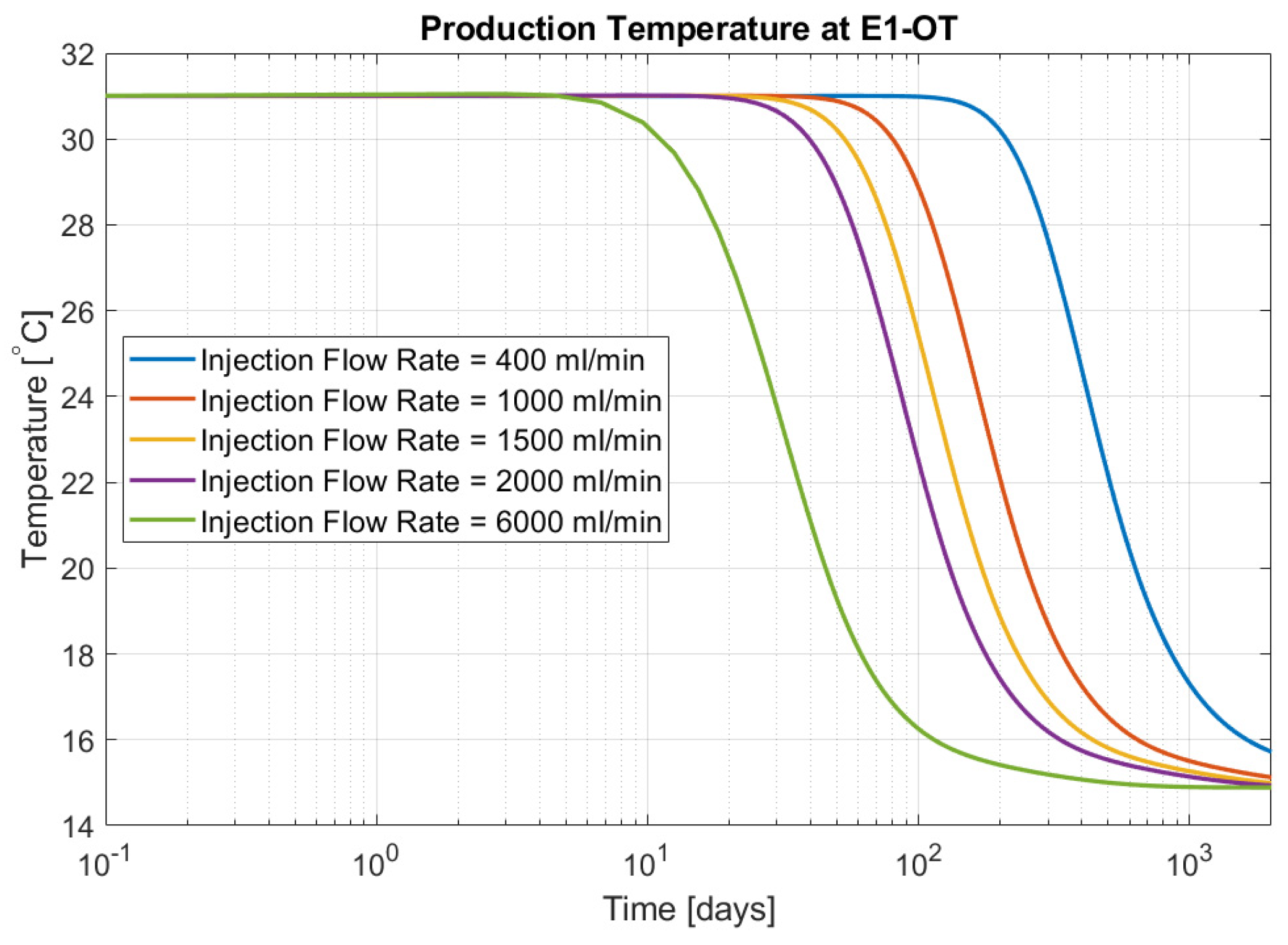
5.3. Coupled TH Model with EDFM for Tracer Transport

Ref. [42] modified the THM model to include the dynamic adsorption features for tracer transport. The adsorption is usually computed by adding a model to the accumulation terms in Equation (2):

$${\displaystyle \frac{\partial M^{\kappa }}{\partial t}}={\displaystyle \frac{\partial \left(\varphi {\sum }_{\beta }{S}_{\beta }{\rho }_{\beta }{X}_{\beta }^{\kappa }\right)}{\partial t}}+{\delta }_{\beta }{\displaystyle \frac{\partial \left(\left(1-\varphi \right){\mathsf{\Gamma }}_{\kappa }\right)}{\partial t}}$$

(69)

where ${\mathsf{\Gamma }}_{\kappa }$ is the adsorption mass per unit rock volume and ${\delta }_{\beta }$ is the Kronecker delta.

The adsorption mass per unit rock volume has various forms for different models. Henry’s law describes a linear adsorption:

$${\mathsf{\Gamma }}_{\kappa }=k{\rho }_{\beta }{S}_{\beta }{X}_{\beta }^{\kappa }$$

(70)

in which $k$ is the linear slope for Henry’s law. The Langmuir equilibrium model can be computed by the following:

$${\mathsf{\Gamma }}_{\mathsf{\kappa }}={\displaystyle \frac{Q_{a}K{\rho }_{\beta }{S}_{\beta }{X}_{\beta }^{\kappa }}{1+K{\rho }_{\beta }{S}_{\beta }{X}_{\beta }^{\kappa }}}$$

(71)

in which $Q_a$ is the ‘saturated’ concentration that this model will approach when concentration is very high and $K$ is equilibrium coefficient for the Langmuir model. Kinetic models involve a dynamic term, such as the Langmuir kinetic model:

$${\displaystyle \frac{d{\mathsf{\Gamma }}_{\mathsf{\kappa }}}{dt}}=k_a{\rho }_{\beta }{S}_{\beta }{X}_{\beta }^{\kappa }\left(Q_a-{\mathsf{\Gamma }}_{\mathsf{\kappa }}\right)-k_d{\mathsf{\Gamma }}_{\mathsf{\kappa }}$$

(72)

in which $k_a$ and $k_d$ are rate constants for forward and reverse processes. Two-site models can be governed by the following:

$${\displaystyle \frac{d{\mathsf{\Gamma }}_1}{dt}}=k_{a1}\widehat{c}\left(Q_{a1}-{\mathsf{\Gamma }}_1\right)-k_{d1}{\mathsf{\Gamma }}_1$$

(73)

$${\displaystyle \frac{d{\mathsf{\Gamma }}_2}{dt}}=k_{a2}\widehat{c}\left(Q_{a2}-{\mathsf{\Gamma }}_2\right)-k_{d2}{\mathsf{\Gamma }}_2$$

(74)

This model consists of two kinetic models for two adsorption sites and a similar model is called a bilayer model where the adsorption of one site is dependent on the adsorption condition of the other site:

$${\displaystyle \frac{d{\mathsf{\Gamma }}_1}{dt}}=k_{a1}\widehat{c}\left(Q_{a1}-{\mathsf{\Gamma }}_1\right)-k_{d1}{\mathsf{\Gamma }}_1$$

(75)

$${\displaystyle \frac{d{\mathsf{\Gamma }}_2}{dt}}=k_{a2}\widehat{c}\left(Q_{a2}{\displaystyle \frac{{\mathsf{\Gamma }}_1}{Q_{a1}}}-{\mathsf{\Gamma }}_2\right)-k_{d2}{\mathsf{\Gamma }}_2$$

(76)

In these two-site models, concentration can be expressed by the following:

$$\widehat{c}=\left[\begin{array}{cc}{\rho }_{\beta }{S}_{\beta }{X}_{\beta }^{\kappa }& {\rho }_{\beta }{S}_{\beta }{X}_{\beta }^{\kappa }<C_{cmc}\\ C_{cmc}& {\rho }_{\beta }{S}_{\beta }{X}_{\beta }^{\kappa }\ge C_{cmc}\end{array}\right.$$

(77)

The dynamic models have been validated by [42] using published or existing models or experimental results. Embedded discrete fracture models are also used but geomechanics are not considered in this study. However, geomechanics for EDFM and reservoir matrix are ready to be used to investigate their impact on tracer transport in this model.

EGS Collab SIGMA-V project is a multi-lab and university collaborative research project in which stimulation, fluid flow and heat transfer processes are investigated at a scale of 10–20 m in the Sanford Underground Research Facility (SURF) in South Dakota. Field-scale experiments are all characterized and monitored by geophysical, hydrological, and geomechanical techniques, which provides the comparison between test and simulation results. The geological condition near the injection and production well is shown in the left part of Figure 15. A hydraulically induced fracture and two natural fractures that intersect with the hydraulic fracture were monitored and characterized by geophysical tools.

A reservoir model with embedded discrete fractures is shown in the right part of Figure 15. Six wells are marked in the reservoir model. E1-I is an injection well and E1-OT, E1-PI, E1-PST, E1-PB, and E1-PDT are production wells. The dimension of the reservoir model is 61 m × 61 m × 49 m, and the discretized mesh contains 61 m × 61 m × 49 m cubes. Natural fractures and the hydraulic fracture are vertical embedded discrete fractures. The hydraulic fracture is 18 m in height (z-direction) and 21 m in length. One natural fracture is 31 m in height (z-direction) and 41 m in length, and the other natural fracture is 31 m in height (z-direction) and 48 m in length. Input parameters are shown in

Table 5. Input parameters for the tracer test in the geothermal reservoir of SURF.

Parameter	Value	Unit
Fracture aperture	0.0001	m
Initial pressure	6.895	MPa
Tracer injection rate	2.91 × 10−4	${\displaystyle \frac{\mathrm{kg}}{\mathrm{s}}}$
Tracer injection time	360	s
Water injection rate	6.667 × 10−4	${\displaystyle \frac{\mathrm{kg}}{\mathrm{s}}}$
Matrix permeability	8.0 × 10−16	${\mathrm{m}}^2$
Fracture permeability (layer 1–22)	2.333 × 10−10	${\mathrm{m}}^2$
Fracture permeability (Layer 23–49)	1.333 × 10−10	${\mathrm{m}}^2$
Reservoir temperature	31	°C
Injected water temperature	15	°C

.

Results from simulation and in situ experimental measurements are shown in Figure 16. It can be observed that although the concentration units are not the same in the two plots, the breakthrough curves have the same shape and the concentration peak time matched very well. The agreement further proves the geometry of characterized fractures close to the real condition. The capability of tracer transport in the coupled THM model is demonstrated. A simulation of thermal breakthrough is also performed—injection into E1-I and production from well E1-OT, as shown in Figure 17. Higher injection flow rate results in earlier thermal breakthrough.

6. Summary and Conclusions

This paper reviews and continues the THM modeling studies in [12,25,32,42]. The coupled THM model used in their work are extended based on a similar program framework. The approach of coupling geomechanics into a thermal and hydraulic model has been discussed: the poro-thermo-elastic Navier equation is chosen to be the mechanical governing equation, which is discretized by the IFD method. This coupling scheme reduces the effort of modifying the original codes for modeling thermal and hydraulic processes due to the fact that mass and energy balance equations are discretized by the same IFD method and grid as well. Validation of the coupled THM model is illustrated in this paper as well as in the original studies.

The coupled THM model and resulting numerical approach, based on the mean stress formulation, have several distinguished advantages and enhancements over existing coupled THM reservoir modeling methodologies in the literature. These advances and improvements with this mean-stress-based THM model include (a) providing rigorous and accurate solutions for fully coupled THM processes in reservoirs by solving all governing equations with the same numerical approach simultaneously and fully implicitly on the same grid; (b) overcoming the intrinsic mass and energy conservation issues inherently with a commonly used one-way sequential coupling approach; (c) avoiding inefficient, difficult linkage between reservoir simulators and geomechanical codes from different developers in general; (d) being able to obtain the entire stress tensor accurately for geomechanical calculations; (e) being able to handle various types of fractures; and (f) being more computationally efficient for handling large-scale, 3D field modeling studies. In short, the mean stress THM model is recommended for use in all reservoir simulations where the goal is fluid and heat flow or mass and energy conservation and transport, and rock mechanical properties are correlated to mean stress, such as for an EGS reservoir.

In the developed coupled THM model, several new features are developed and incorporated, such as fracture aperture expansion due to temperature drop in a double-porosity model, coupled fracture mechanics including thermal stresses in an EDFM approach, and tracer transport using dynamic adsorption models. This is needed for model application in geothermal reservoir simulation where geomechanical and thermal impact cannot be neglected. The mathematical model adopted for these features is presented in this paper and the application of the coupled THM model is demonstrated for field-scale geothermal reservoir simulation. Fracture aperture enhancement and geomechanical and thermal stress impact are assessed in this paper. Another application of tracer transport into a real field-scale geothermal reservoir is also discussed for the capability of simulating transport phenomena using the coupled TH model.

In this paper, modeling results show that thermally induced geomechanic effects have a significant impact on EGS reservoir development, mainly by significantly altering the fracture aperture and permeability. The coupled THM model introduced in this paper is capable of capturing such effects. Moreover, our model can be easily extended to incorporate additional features or mechanisms that better describe the physics related with fluid and heat flow and geomechanics in EGS reservoirs.

References

1. Gens, A.; Guimaräes, L.D.N.; Olivella, S.; Sánchez, M. Modelling Thermo-Hydro-Mechano-Chemical Interactions for Nuclear Waste Disposal. J. Rock Mech. Geotech. Eng. 2010, 2, 97–102. [Google Scholar] [CrossRef]
2. Huang, Z.-Q.; Winterfeld, P.H.; Xiong, Y.; Wu, Y.-S.; Yao, J. Parallel Simulation of Fully-Coupled Thermal-Hydro-Mechanical Processes in CO2 Leakage through Fluid-Driven Fracture Zones. Int. J. Greenh. Gas Control 2015, 34, 39–51. [Google Scholar] [CrossRef]
3. Cappa, F.; Rutqvist, J. Modeling of Coupled Deformation and Permeability Evolution during Fault Reactivation Induced by Deep Underground Injection of CO2. Int. J. Greenh. Gas Control 2011, 5, 336–346. [Google Scholar] [CrossRef]
4. Lei, H.; Xu, T.; Jin, G. TOUGH2Biot—A Simulator for Coupled Thermal-Hydrodynamic-Mechanical Processes in Subsurface Flow Systems: Application to CO2 Geological Storage and Geothermal Development. Comput. Geosci. 2015, 77, 8–19. [Google Scholar] [CrossRef]
5. Rutqvist, J. Status of the TOUGH-FLAC Simulator and Recent Applications Related to Coupled Fluid Flow and Crustal Deformations. Comput. Geosci. 2011, 37, 739–750. [Google Scholar] [CrossRef]
6. Taron, J.; Elsworth, D. Thermal-Hydrologic-Mechanical-Chemical Processes in the Evolution of Engineered Geothermal Reservoirs. Int. J. Rock Mech. Min. Sci. 2009, 46, 855–864. [Google Scholar] [CrossRef]
7. Yao, J.; Zhang, X.; Sun, Z.; Huang, Z.; Liu, J.; Li, Y.; Xin, Y.; Yan, X.; Liu, W. Numerical Simulation of the Heat Extraction in 3D-EGS with Thermal-Hydraulic-Mechanical Coupling Method Based on Discrete Fractures Model. Geothermics 2018, 74, 19–34. [Google Scholar] [CrossRef]
8. Taron, J.; Elsworth, D. Coupled Mechanical and Chemical Processes in Engineered Geothermal Reservoirs with Dynamic Permeability. Int. J. Rock Mech. Min. Sci. 2010, 47, 1339–1348. [Google Scholar] [CrossRef]
9. Taron, J.; Elsworth, D.; Min, K.-B. Numerical Simulation of Thermal-Hydrologic-Mechanical-Chemical Processes in Deformable, Fractured Porous Media. Int. J. Rock Mech. Min. Sci. 2009, 46, 842–854. [Google Scholar] [CrossRef]
10. Pandey, S.N.; Chaudhuri, A.; Kelkar, S. A Coupled Thermo-Hydro-Mechanical Modeling of Fracture Aperture Alteration and Reservoir Deformation during Heat Extraction from a Geothermal Reservoir. Geothermics 2017, 65, 17–31. [Google Scholar] [CrossRef]
11. Hofmann, H.; Babadagli, T.; Yoon, J.S.; Blöcher, G.; Zimmermann, G. A Hybrid Discrete/Finite Element Modeling Study of Complex Hydraulic Fracture Development for Enhanced Geothermal Systems (EGS) in Granitic Basements. Geothermics 2016, 64, 362–381. [Google Scholar] [CrossRef]
12. Wang, S.; Huang, Z.; Wu, Y.-S.; Winterfeld, P.H.; Zerpa, L.E. A Semi-Analytical Correlation of Thermal-Hydraulic-Mechanical Behavior of Fractures and Its Application to Modeling Reservoir Scale Cold Water Injection Problems in Enhanced Geothermal Reservoirs. Geothermics 2016, 64, 81–95. [Google Scholar] [CrossRef]
13. Cao, W.; Huang, W.; Jiang, F. A Novel Thermal–Hydraulic–Mechanical Model for the Enhanced Geothermal System Heat Extraction. Int. J. Heat Mass Transf. 2016, 100, 661–671. [Google Scholar] [CrossRef]
14. Garipov, T.T.; Tomin, P.; Rin, R.; Voskov, D.V.; Tchelepi, H.A. Unified Thermo-Compositional-Mechanical Framework for Reservoir Simulation. Comput. Geosci. 2018, 22, 1039–1057. [Google Scholar] [CrossRef]
15. Pandey, S.N.; Vishal, V.; Chaudhuri, A. Geothermal Reservoir Modeling in a Coupled Thermo-Hydro-Mechanical-Chemical Approach: A Review. Earth-Sci. Rev. 2018, 185, 1157–1169. [Google Scholar] [CrossRef]
16. Kim, J.; Tchelepi, H.A.; Juanes, R. Stability, Accuracy and Efficiency of Sequential Methods for Coupled Flow and Geomechanics. In Proceedings of the SPE Reservoir Simulation Symposium: Society of Petroleum Engineers, The Woodlands, TX, USA, 2–4 February 2009. [Google Scholar]
17. Jha, B.; Juanes, R. A Locally Conservative Finite Element Framework for the Simulation of Coupled Flow and Reservoir Geomechanics. Acta Geotech. 2007, 2, 139–153. [Google Scholar] [CrossRef]
18. Min, K.-B.; Rutqvist, J.; Tsang, C.-F.; Jing, L. Stress-Dependent Permeability of Fractured Rock Masses: A Numerical Study. Int. J. Rock Mech. Min. Sci. 2004, 41, 1191–1210. [Google Scholar] [CrossRef]
19. Rutqvist, J.; Wu, Y.-S.; Tsang, C.-F.; Bodvarsson, G. A Modeling Approach for Analysis of Coupled Multiphase Fluid Flow, Heat Transfer, and Deformation in Fractured Porous Rock. Int. J. Rock Mech. Min. Sci. 2002, 39, 429–442. [Google Scholar] [CrossRef]
20. Kim, J.; Tchelepi, H.A.; Juanes, R. Stability and Convergence of Sequential Methods for Coupled Flow and Geomechanics: Fixed-Stress and Fixed-Strain Splits. Comput. Methods Appl. Mech. Eng. 2011, 200, 1591–1606. [Google Scholar] [CrossRef]
21. Dean, R.H.; Gai, X.; Stone, C.M.; Minkoff, S.E. A Comparison of Techniques for Coupling Porous Flow and Geomechanics. SPE J. 2006, 11, 132–140. [Google Scholar] [CrossRef]
22. Mikelić, A.; Wheeler, M.F. Convergence of Iterative Coupling for Coupled Flow and Geomechanics. Comput. Geosci. 2013, 17, 455–461. [Google Scholar] [CrossRef]
23. Wang, W.; Kosakowski, G.; Kolditz, O. A Parallel Finite Element Scheme for Thermo-Hydro-Mechanical (THM) Coupled Problems in Porous Media. Comput. Geosci. 2009, 35, 1631–1641. [Google Scholar] [CrossRef]
24. Hu, L.; Winterfeld, P.H.; Fakcharoenphol, P.; Wu, Y.-S. A Novel Fully-Coupled Flow and Geomechanics Model in Enhanced Geothermal Reservoirs. J. Pet. Sci. Eng. 2013, 107, 1–11. [Google Scholar] [CrossRef]
25. Winterfeld, P.H.; Wu, Y.-S. Simulation of Coupled Thermal/Hydrological/Mechanical Phenomena in Porous Media. SPE J. 2016, 21, 1041–1049. [Google Scholar] [CrossRef]
26. Yu, X.; Wang, S.; Wu, Y.-S. Performance Evaluation of a Physics-Based Multi-Stage Preconditioner in Numerical Simulation of Coupled Fluid and Heat Flow in Porous Media. In Proceedings of the 44th Stanford Geothermal Workshop Proceedings, Stanford, CA, USA, 11–13 February 2019. [Google Scholar]
27. Lacroix, S.; Vassilevski, Y.V.; Wheeler, M.F. Decoupling Preconditioners in the Implicit Parallel Accurate Reservoir Simulator (IPARS). Numer. Linear Algebra Appl. 2001, 8, 537–549. [Google Scholar] [CrossRef]
28. Cusini, M.; Lukyanov, A.A.; Natvig, J.; Hajibeygi, H. Constrained Pressure Residual Multiscale (CPR-MS) Method for Fully Implicit Simulation of Multiphase Flow in Porous Media. J. Comput. Phys. 2015, 299, 472–486. [Google Scholar] [CrossRef]
29. Cao, H.; Tchelepi, H.A.; Wallis, J.R.; Yardumian, H.E. Parallel Scalable Unstructured CPR-Type Linear Solver for Reservoir Simulation. In Proceedings of the SPE Annual Technical Conference and Exhibition: Society of Petroleum Engineers, Dallas, TX, USA, 9–12 October 2005. [Google Scholar]
30. Liu, H.; Wang, K.; Chen, Z.; Jordan, K.E. Efficient Multi-Stage Preconditioners for Highly Heterogeneous Reservoir Simulations on Parallel Distributed Systems. In Proceedings of the SPE Reservoir Simulation Symposium: Society of Petroleum Engineers, Houston, TX, USA, 23–25 February 2015. [Google Scholar]
31. Winterfeld, P.H.; Wu, Y.-S. A Novel Fully Coupled Geomechanical Model for CO2 Sequestration in Fractured and Porous Brine Aquifers. In Proceedings of the XIX International Conference on Water Resources: University of Illinois at Urbana-Champagne, Urbana, IL, USA, 17–21 June 2012. [Google Scholar]
32. Yu, X.; Winterfeld, P.; Wang, S.; Wang, C.; Wang, L.; Wu, Y. A Geomechanics-Coupled Embedded Discrete Fracture Model and Its Application in Geothermal Reservoir Simulation. In Proceedings of the SPE Reservoir Simulation Conference: Society of Petroleum Engineers, Galveston, TX, USA, 10–11 April 2019. [Google Scholar]
33. Warren, J.E.; Root, P.J. The Behavior of Naturally Fractured Reservoirs. Soc. Pet. Eng. J. 1963, 3, 245–255. [Google Scholar] [CrossRef]
34. Kazemi, H.; Merrill, L.S.; Porterfield, K.L.; Zeman, P.R. Numerical Simulation of Water-Oil Flow in Naturally Fractured Reservoirs. Soc. Pet. Eng. J. 1976, 16, 317–326. [Google Scholar] [CrossRef]
35. Wu, Y.-S. On the Effective Continuum Method for Modeling Multiphase Flow, Multicomponent Transport, and Heat Transfer in Fractured Rock. Am. Geophys. Union (AGU) 2000, 122, 299–312. [Google Scholar]
36. Moinfar, A.; Varavei, A.; Sepehrnoori, K.; Johns, R.T. Development of a Coupled Dual Continuum and Discrete Fracture Model for the Simulation of Unconventional Reservoirs. In Proceedings of the SPE Reservoir Simulation Symposium: Society of Petroleum Engineers, The Woodlands, TX, USA, 18–20 February 2013. [Google Scholar]
37. Lee, S.H.; Lough, M.F.; Jensen, C.L. Hierarchical Modeling of Flow in Naturally Fractured Formations with Multiple Length Scales. Water Resour. Res. 2001, 37, 443–455. [Google Scholar] [CrossRef]
38. Li, L.; Lee, S.H. Efficient Field-Scale Simulation for Black Oil in a Naturally Fractured Reservoir via Discrete Fracture Networks and Homogenized Media. In Proceedings of the International Oil & Gas Conference and Exhibition in China: Society of Petroleum Engineers, Beijing, China, 5–7 December 2006. [Google Scholar]
39. Horne, R.N.; Rodriguez, F. Dispersion in Tracer Flow in Fractured Geothermal Systems. Geophys. Res. Lett. 1983, 10, 289–292. [Google Scholar] [CrossRef]
40. Kocabas, I. Geothermal Reservoir Characterization via Thermal Injection Backflow and Interwell Tracer Testing. Geothermics 2005, 34, 27–46. [Google Scholar] [CrossRef]
41. Shook, G.M. Predicting Thermal Breakthrough in Heterogeneous Media from Tracer Tests. Geothermics 2001, 30, 573–589. [Google Scholar] [CrossRef]
42. Winterfeld, P.; Johnston, B.; Beckers, K.; Wu, Y.-S.; The EGS Collab Team. Code Modifications for Modeling Chemical Tracers and Embedded Natural Fractures at EGS Collab. In Proceedings of the 44th Stanford Geothermal Workshop Proceedings, Stanford, CA, USA, 11–13 February 2019. [Google Scholar]
43. Pruess, K.; Oldenburg, C.; Moridis, G. TOUGH2 User’s Guide, Version 2; Earth Sciences Division, Lawrence Berkeley National Laboratory University of California: Berkeley, CA, USA, 1999. [Google Scholar]
44. Zhang, K.; Wu, Y.-S.; Pruess, K. User’s Guide for TOUGH2-MP—A Massively Parallel Version of the TOUGH2 Code. In LBNL-315E, Earth Sciences Division; Lawrence Berkeley National Laboratory: Berkeley, CA, USA, 2008. [Google Scholar]
45. Jaeger, J.C.; Cook, N.G.W.; Zimmerman, R. Fundamentals of Rock Mechanics; Blackwell Publishing: Oxford, UK, 2007; ISBN 1444308912. [Google Scholar]
46. Winterfeld, P.H.; Wu, Y.-S. An Overview of Our Coupled Thermal-Hydrological-Mechanical Simulator for Porous and Fractured Media. In Proceedings of the ARMA 20-1252, in 54th US Rock Mechanics/Geomechanics Symposium, Golden, CO, USA, 28 June–1 July 2020. [Google Scholar]
47. Winterfeld, P.H.; Wu, Y.-S. Parallel Simulation of CO2 Sequestration with Rock Deformation in Saline Aquifers. In Proceedings of the SPE Reservoir Simulation Symposium: Society of Petroleum Engineers, The Woodlands, TX, USA, 21–23 February 2011. [Google Scholar]
48. Karypis, G.; Kumar, V. A Parallel Algorithm for Multilevel Graph Partitioning and Sparse Matrix Ordering. J. Parallel Distrib. Comput. 1998, 48, 71–85. [Google Scholar] [CrossRef]
49. Karypis, G.; Kumar, V. A Fast and High Quality Multilevel Scheme for Partitioning Irregular Graphs. Siam J. Sci. Comput. 1999, 20, 359–392. [Google Scholar] [CrossRef]
50. Balay, S.; Abhyankar, S.; Adams, M.F.; Brown, J.; Brune, P. PETSc User’s Manual; Argonne National Laboratory: Argonne, IL, USA, 2019. [Google Scholar]
51. Rutqvist, J.; Vasco, D.W.; Myer, L. Coupled Reservoir-Geomechanical Analysis of CO2 Injection and Ground Deformations at In Salah, Algeria. Int. J. Greenh. Gas Control 2010, 4, 225–230. [Google Scholar] [CrossRef]
52. Itasca. FLAC3D, Fast Lagrangian Analysis of Continua in 3-Dimensions, Version 4.0; Itasca Consulting Group: Minneapolis, MN, USA, 2009.
53. Mandel, J. Consolidation Des Sols (Étude Mathématique). Géotechnique 1953, 3, 287–299. [Google Scholar] [CrossRef]
54. Abousleiman, Y.; Cheng, A.H.-D.; Cui, L.; Detournay, E.; Roegiers, J.-C. Mandel’s problem revisited. Géotechnique 1996, 46, 187–195. [Google Scholar] [CrossRef]
55. Witherspoon, P.A.; Wang, J.Y.; Iwai, K.; Gale, J.E. Validity of Cubic Law for Fluid Flow in a Deformable Rock Fracture. Water Resour. Res. 1980, 16, 1016–1024. [Google Scholar] [CrossRef]
56. Carman, P.C. Flow of Gases Through Porous Media; Academic Press: Cambridge, MA, USA, 1956. [Google Scholar]
57. Gutierrez, M.; Lewis, R.W.; Masters, I. Petroleum Reservoir Simulation Coupling Fluid Flow and Geomechanics. SPE Reserv. Eval. Eng. 2001, 4, 164–172. [Google Scholar] [CrossRef]
Figure 1. Net flux of a single grid, left, and the quantities used to describe a connection between two grids, right.
Energies 18 03017 g001
Figure 2. Program structure of the simulator for the coupled THM model.
Energies 18 03017 g002
Figure 3. Comparison of pressure change and surface uplift from results of our simulator [25] and TOUGH2-FLAC [51].
Energies 18 03017 g003
Figure 4. Schematic of the model of Mandel’s problem: load applied on the top and drainage is allowed on the two lateral boundaries [32].
Energies 18 03017 g004
Figure 5. Comparison of analytical and simulated pore pressures at the center of the sample for Mandel’s problem.
Energies 18 03017 g005
Figure 6. Geothermal reservoir model for semi-analytical solution application: left, geothermal reservoir showing locations of fractured rock and caprock; right, top view showing location of injector and producer [12].
Energies 18 03017 g006
Figure 7. Permeability change after cold water injection at 180 days (left) and 7 years (right): y-permeability for this case.
Energies 18 03017 g007
Figure 8. Fracture aperture and permeability variation near cold injector during injection of 7 years.
Energies 18 03017 g008
Figure 9. Fracture permeability change during 7 years of cold water injection under different scenarios of injection temperatures: 70 °C; 80 °C; 90 °C.
Energies 18 03017 g009
Figure 10. Schematic plot for EDFM and geomechanics coupling: red and green planes represent fracture elements and box stands for primary grid; blue arrows are stress components for primary grids and yellow arrows are thermal stress and net effective stress.
Energies 18 03017 g010
Figure 11. Schematic model of geothermal reservoir with an injector and a producer, plus six long discrete fractures. The fractures allow flow to occur from the injector to the producer.
Energies 18 03017 g011
Figure 12. Pressure and temperature distribution after injection/production for 500 days: (a) results for coupled THM model; (b) results for TH model without geomechanics.
Energies 18 03017 g012
Figure 13. Flow rate and production temperature comparison for two cases: with geomechanics coupling; without geomechanics coupling. Production temperature (thermal breakthrough) is influenced by considering geomechanics.
Energies 18 03017 g013
Figure 14. Fracture permeability at an observation point: relation with time (left) and temperature (right).
Energies 18 03017 g014
Figure 15. Schematic plot for the fractures, wells, and drift at the geothermal field of SURF (left); cross-section of embedded discrete fracture model set up for tracer transport simulation that includes the hydraulic fracture (vertical one) connecting two wells (right) and the two natural fractures.
Energies 18 03017 g015
Figure 16. Tracer breakthrough curves modeled by simulation (left) and obtained by experiments (right). The units in two plots are different. The forms of both are similar.
Energies 18 03017 g016
Figure 17. Thermal breakthrough curve under different injection flow rates.
Energies 18 03017 g017