Numerical Assessment of a Heavy-Duty (HD) Spark Ignition (SI) Biogas Engine

Abstract

This paper examines the feasibility of converting a Heavy-Duty (HD) Spark Ignition (SI) Compressed Natural Gas (CNG) engine to biogas fuel. A One-Dimensional (1D) simulation tool was used to model a commercially available HD SI CNG engine. The model was validated by comparing experimental and computed in-cylinder pressure, brake power, fuel, and air mass flow rates. The engine was then modified to use biogas with an injection system based on existing designs from the literature. A Spark Advance (SA) sweep was performed to assess the engine’s performance at full load. The chosen equivalence ratio was 0.85, and the engine speed was 1500 rpm. The Maximum Brake Power (MBP) and Maximum Brake Efficiency (MBE) operating points were identified. Partial load analysis was conducted starting from the MBP conditions. Results in terms of brake power, brake efficiency, and NO_x emissions are presented. Conversion to biofuel results in a reduction in power and efficiency of 33% and 4%, respectively, at 1500 rpm and full load conditions. Brake Specific NO_x emissions remained comparable. This numerical study demonstrates the feasibility of biogas conversion for HD SI engines, offering a renewable fuel alternative to reduce greenhouse gas emissions, though with trade-offs in power and efficiency.

1. Introduction

Biogas and biomethane production have a large role in the context of emission reduction promoted by the European Union (EU) and in reducing the energy dependency on foreign countries. Indeed, an increase in biomethane production to 33 billion cubic meters per year in 2030 would save around 110 Mtonne of equivalent carbon dioxide CO₂ [1]. This would account for ca. 6% of the required effort to reach the target of 55% Greenhouse Gas (GHG) reduction presented in the European Commission’s Fit for 55 package [2]. Indeed, replacing fossil fuels with biomethane typically leads to a GHG emission reduction of 80%. This can also increase to 200% when considering the removal of GHG from the atmosphere (with carbon capture for example) or the avoided emissions associated with the usage of specific feedstocks that would otherwise be wasted. For example, by using manure, it is possible to avoid methane (CH₄) and nitrogen oxide (NO_x) emissions that would occur if left untreated [1].

The main biomethane/biogas production pathway is the anaerobic digestion of waste and residual biomass. In the production plants, the feedstock is sent into biogas digesters where microorganisms break down the organic matter. These produce a blend of gases with varying percentages of CH₄ and CO₂. The typical composition of biogas ranges between 45 and 85% of CH₄ and 15–55% of CO₂ on a volume basis [3]. The gas produced can be used for a variety of applications. It can be burnt directly in Combined Heat and Power (CHP) plants, thus providing thermal and electrical energy [4,5]. Another use is as feedstock for different chemical processes. For example, to produce fuel such as diesel, gasoline, and methanol via the Fischer–Tropsch process [6,7]. Some studies also foresee biogas utilization in Fuel Cells (FCs) to produce electricity [8,9] or in CHP configurations as presented in [10]. Lastly, biogas can be purified by removing impurities, such as hydrogen sulfide, and the CO₂ present in it. This is called “biogas upgrading”. The upgrading processes produce biomethane that can substitute fossil natural gas. Upgrading plants typically rely on membranes [11] or water scrubbing, chemical absorption, and pressure swing adsorption [12] to separate CO₂ from CH₄. The upgraded biogas can then be directly injected into the distribution grid, reducing the quantity of methane from fossil sources [13].

Biogas production and upgrading plants require both electricity and heat for chemical processes and delivery of products. These energy streams can be provided with different technologies, as presented in [11]. For example, when used in a CHP configuration, an Internal Combustion Engine (ICE) integrated into the system could fulfill both electrical and heat loads needed by the plant. In addition, using ICEs could be especially relevant in off-grid plants based on electrified steam methane reforming for the syngas production process. An example of such a commercially available plant is presented in [14], albeit this uses electricity from renewable sources to power the reactor. Indeed, a recent paper [15] shows that these kinds of production plants are usually oversized when set up to be grid-independent and rely only on renewable energy and batteries, leading to higher capital costs. Moreover, in some operating conditions dependent on the availability of the renewable source, the energy produced could be curtailed up to almost 80%. The integration of an ICE would add another degree of flexibility, as it would substitute renewable energy sources and batteries in low-energy availability scenarios.

Several studies have investigated the effects of using syngas or biogas with a high content of CO₂ in a Spark Ignition (SI) engine, focusing on assessing and comparing the performance of conventional ICEs fueled with various mixtures of CO₂ and CH₄. Huang et al. [16] explored the impact of varying Compression Ratios (CRs), engine speeds, equivalence ratios, and fuel mixtures on Single Cylinder Engine (SCE) performance. They found that higher CO₂ contents degraded engine performance, but an increased CR could mitigate the negative effects of CO₂-rich fuel. However, they observed knock at CRs above 15:1. Byun et al. [17] conducted experimental and numerical simulations on a turbocharged Light-Duty (LD) SCE under stoichiometric and lean conditions. Their results show that increasing CO₂ content led to decreased engine performances, but also reduced NO_x production due to the lower combustion temperatures. A similar work was presented by Kim et al. in [18]. They analyzed a three-cylinder SI engine at various loads, equivalence ratios, and CO₂/CH₄ blend ratios but with a fixed value of Spark Advance (SA). They observed worsened combustion performance with higher CO₂ levels, including lower peak cylinder pressures and delayed and broader combustion durations. These studies provide valuable experimental and numerical insights for low-power engines fueled with biogas with different CO₂ and CH₄ contents suited for gensets or LD applications. However, to the best of the authors’ knowledge, no experimental nor numerical investigations have examined Heavy-Duty (HD) SI engines. For this reason, it is the interest of the authors to numerically assess the possibility of conversion of an HD SI Compressed Natural Gas (CNG) engine to run on biogas in the specific context of being integrated into a large-scale biogas production plant.

The virtual conversion of a conventional HD SI CNG engine to operate on biogas was achieved using ICE One-Dimensional (1D) simulation tools. Initially, the CNG engine was modeled and validated against experimental data. Subsequently, the engine configuration was modified with minimal changes to use biogas. For the modified configuration, two full-load operating points were identified through an SA sweep maintaining the wastegate valve of the Turbo-Charger (TC) completely closed. These points represent the Maximum Brake Power (MBP) and Maximum Brake Efficiency (MBE) operating conditions. Partial load simulations were then conducted from the full load at MBP to better understand the engine performance in these conditions. Load reduction was primarily achieved by opening the Wastegate (WG) valve and, at very low loads, by closing the throttle valve. The value of SA, equivalence ratio, and engine speed were kept constant at their full-load settings.

The paper is structured as follows. First, the modeling and validation of an HD SI CNG engine using a 1D simulation tool are presented and discussed. The third Section details the necessary modifications to the baseline engine configuration to enable biogas conversion, with the choice of the full load operating points. In the fourth Section, partial load simulations of the converted engine are presented. Results for full and partial load operating conditions are then shown and discussed. At last, CNG and biogas-fueled engine performances are compared for the full load operations at the same regime.

2. CNG Engine Modeling and Validation

The engine chosen for this study is a 6-cylinder, 13 L HD engine available in various fueling configurations, such as diesel and CNG. The main characteristics of the CNG configuration are summarized in

Table 1. HD SI CNG-fueled engine specification.

Configuration	Inline 6 cyl.
Bore	135	mm
Stroke	150	mm
Connecting rod length	230	mm
IVC	−141	CAD aTDC
EVO	120	CAD aTDC
Displacement	13	L
CR	12:1
Fuel	CNG
Fuel injection system	Multi-Point
TC system	Fixed geometry turbine with WG
Ignition system	SI
Max power	338 @ 1900 rpm	kW
Max torque	2000 @ 1100 rpm	Nm

, which also include the values of Intake Valve Closing (IVC) and Exhaust Valve Opening (EVO) timings measured in Crank Angle Degrees after Top Dead Center (CAD aTDC).

This engine is typically used in road transport and off-road vehicle applications. However, it represents a possible stationary power generation solution if properly modified.

2.1. Engine Modeling

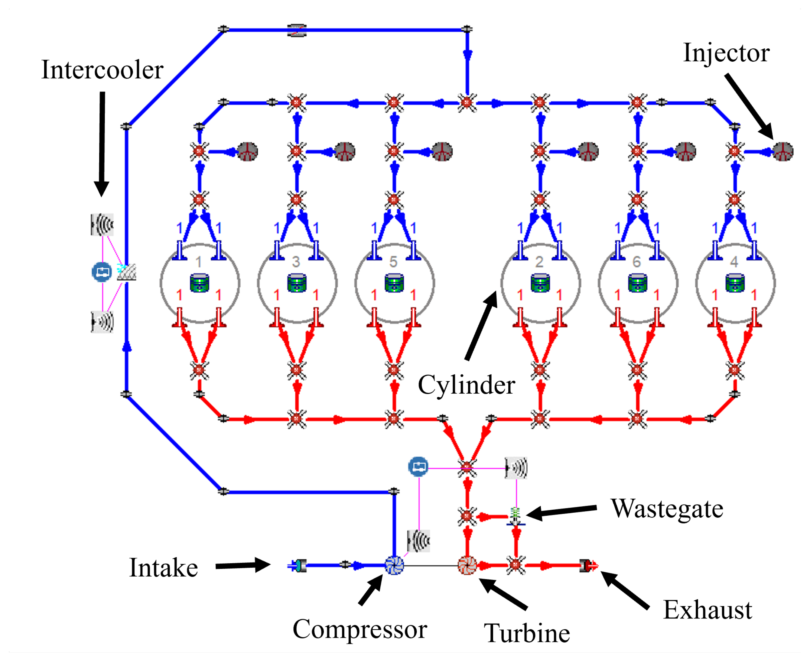
The complete modeling of the engine was made possible using the Gasdyn software (Ver 1.01.1) developed by the ICE Group at Politecnico di Milano. A 1D approach was chosen due to the need for a fast but reliable way to simulate the complete engine in different operating conditions. A visual representation of the virtual engine is reported in Figure 1. Intake and exhaust systems, complete with the Multi-Point (MP) injection system and TC were included in the scheme to reproduce the physical engine with high fidelity.

Intake and exhaust ducts’ fluid dynamic was simulated using a second-order accuracy upwind numerical method presented in [19]. Chemical species conservation equations were considered in addition to the mass, momentum, and energy to account for the effect of gaseous Port Fuel Injection (PFI) on Volumetric Efficiency (VE).

The composition and physical properties of the CNG used in this study are reported in

Table 2. Composition and properties of the CNG and biogas used in this study.

Quantity	CNG	Biogas
Vol. comp. CH4	86.8	55	%
Vol. comp. C2H6	7.9	0	%
Vol. comp. C3H8	2.4	0	%
Vol. comp. C4H10	0.7	0	%
Vol. comp. C5H12	0.2	0	%
Vol. comp. CO2	2	45	%
${\alpha }_{\mathit{st}}$	16.04	5.28	kgair/kgfuel
Lower Heating Value (LHV)	47.01	15.42	MJ/kg
Research Octane Number (RON)	120	110 [20]	-
Density at 1 atm, 20 °C	0.78	1.19	kg/m3
Content of C-H-O	21-78-1	24-54-22	%

, compared to the biogas ones used later.

The modeling of the TC was performed via a Zero-Dimensional (0D) approach, based on corrected mass flow rate-pressure ratio maps provided by the manufacturer. Boost pressure ($p_{\mathit{boost}}$) control was implemented with a PID controller that adjusted the WG valve opening to achieve a set target value.

Combustion was simulated via a two-zone predictive model, whose theoretical description is reported in [21]. The burning rate was evaluated via the so-called “eddy burn-up” model presented originally in [22] and later extended by several authors. The correlation used to estimate the laminar flame speed ($S_l$) is the one proposed in [23]

In-cylinder turbulence was modeled via the $K-k-\epsilon$ model presented in [24].

The evolution of chemical species during combustion was estimated using a chemical equilibrium approach based on the temperature of the burnt zone. Nitrogen oxide emissions were calculated using a super-extended Zel’dovich mechanism [25].

2.2. Model Validation

In this Section, simulation results of the original CNG engine are presented and compared with experimental data. The available data regarded full-load operations for different regimes. The simulations of these conditions were performed starting at an engine speed of 600 rpm and increasing it to 1900 rpm. For all operating points, the target $\varphi$ was set equal to 1, as in the real engine.

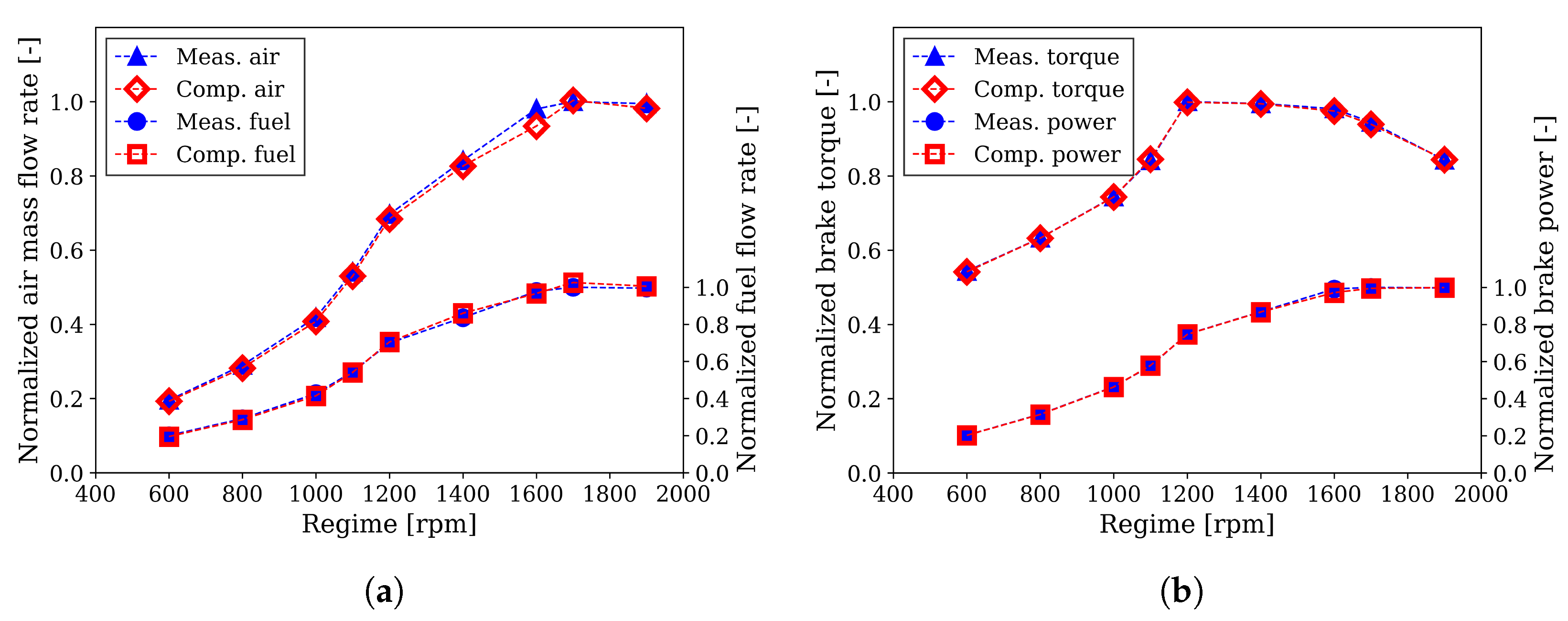
A total of 200 simulation cycles were performed for each simulated point to ensure convergence. Comparisons between normalized experimental and computed values of intake air mass flow rate, fuel mass flow rate, brake torque, and brake power are reported in Figure 2. Normalization was performed with respect to the maximum value of each quantity. This follows a direct request from the manufacturer that provided the data.

Results reported in Figure 2a show that the maximum relative difference between experimental and computed values for the air flow rate is equal to −4.7% at 1600 rpm, while the average one is −1.9%. The maximum relative error for the fuel flow rate is +2.8% at 1400 rpm, and the average is −0.2%. Regarding normalized brake power and torque reported in Figure 2b, the average errors are equal to 0.3% for the former and 0.1% for the latter.

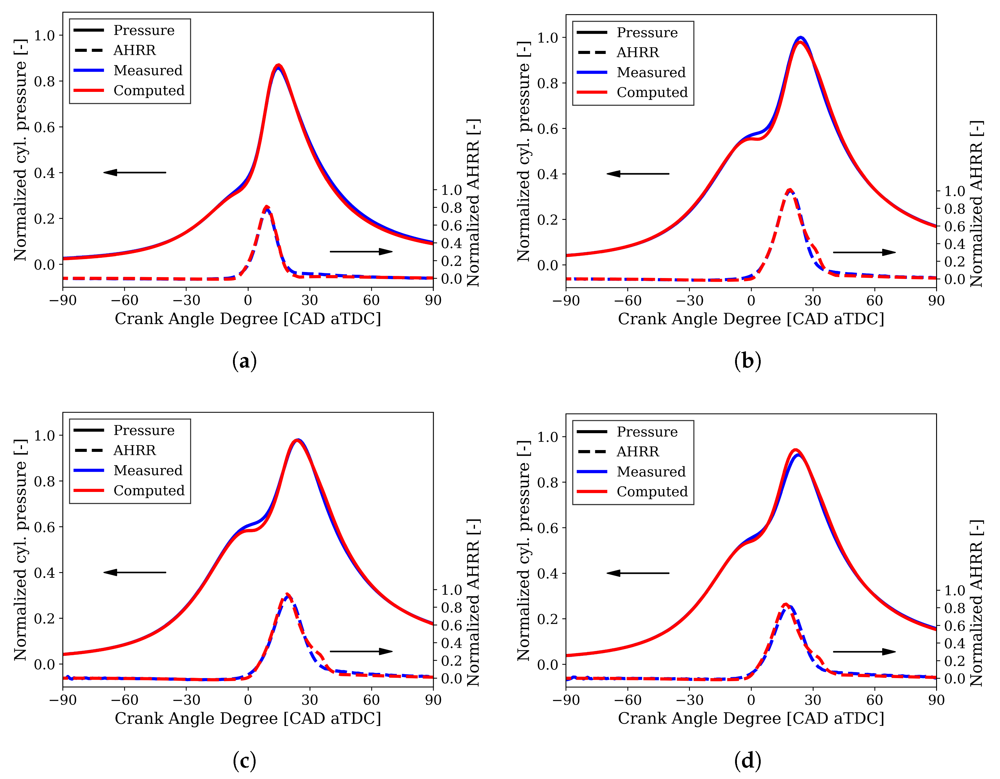
In addition to these quantities, comparisons of normalized in-cylinder pressure traces and Apparent Heat Release Rate (AHRR) for four operating points at different engine speeds are reported in Figure 3. Normalization is relative to the maximum in-cylinder pressure and AHRR values observed experimentally.

The in-cylinder pressure traces in Figure 3 show that the computed values represent the experimental ones from both qualitative and quantitative perspectives. The peak pressure positions and magnitudes are accurately predicted, with an average error on the latter quantity equal to 1.1%. Furthermore, the alignment between the experimental and computed AHRR trends further validates the predictive accuracy of the combustion model employed in this study. The AHRR profiles exhibit strong agreement throughout the combustion process, diverging only slightly during the final stages.

For these simulations, a unique set of tuning parameters for combustion and turbulence models was identified and used for all regimes. SA values were changed according to experimental values. Indeed, the CNG-fueled version of the engine is well simulated, as discussed previously. Hence, this virtual model was used as a starting point to obtain a biogas-fueled configuration with some appropriate modifications. These will be explained in detail in the following section.

3. Biogas-Fueled Engine

In this Section, the necessary modifications to convert the baseline engine to run with biogas are introduced and integrated into the virtual model. Following this, results obtained from full and partial load simulations are presented and discussed.

3.1. Engine Configuration Modifications

The conversion of HD engines usually starts from diesel-fueled ICEs. These can be converted to dual fuel operations [26], in which diesel fuel is still used to ignite the premixed air-fuel charge, or to pure SI operations. In the latter case, several modifications are necessary. These typically include a reduction in CR to avoid auto-ignition (knock), the introduction of a port fuel injection system to obtain complete mixing of fuel and air in the intake pipes, an ignition system (spark plugs), and a throttle valve to regulate the load [27,28]. However, in this study, only the injection system has to be modified as the baseline engine uses a gaseous fuel as well and already has spark plugs to ignite the air–fuel mixture.

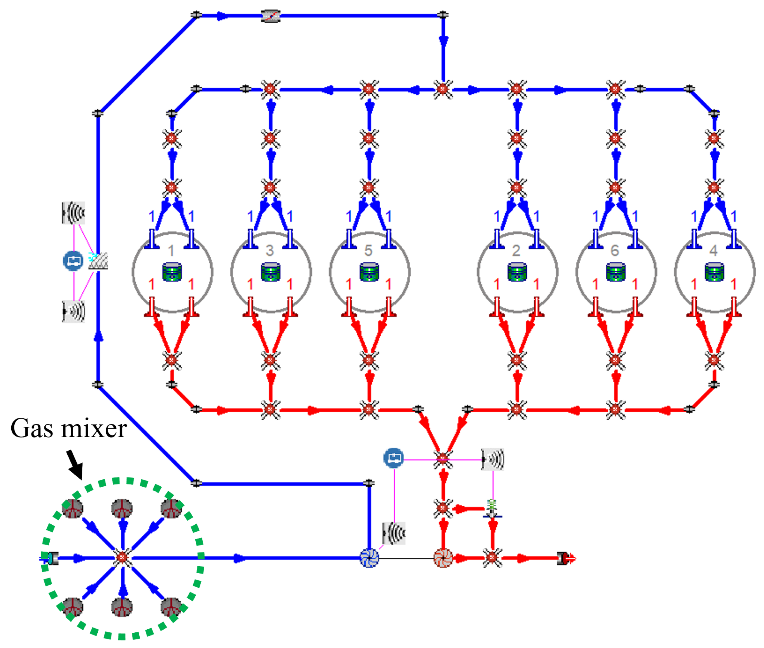
An air–gas mixer had to be introduced in the engine scheme. Two types of mixers are reported and studied in the literature: the non-Venturi [28] and Venturi [29] designs. The latter relies on the Venturi effect with a convergent–divergent tube design that draws in the intake system gaseous fuel from one or several pipes connected to the fuel tank. A detailed Computational Fluid Dynamic (CFD) simulation of these devices, like the one presented in [30], is outside this paper’s scope. However, the effect on VE and air flow rate of the injection system had to be included to provide realistic results. To model the gas mixer, six gaseous fuel injectors were connected to the same junction in the intake pipe just before the compressor side of the TC. The main difference between the previous engine configuration and the current one is that all injectors act on the same portion of the intake circuit. In fact, in the CNG engine, single injectors were connected to the specific ducts that led to the corresponding cylinders, and fuel injection was carried out within a defined time interval. In contrast, the new injection system is set up to closely model a gas mixer by imposing a continuous injection profile, with a specific equivalence ratio as a target on the same duct. The implementation of this device in the Gasdyn model is highlighted with a green circle in Figure 4. It is worth noting that the overall length of the intake pipe before the compressor was not altered.

The authors decided not to modify any additional aspects of the original engine to maintain the comparison between the CNG and biogas-fueled configurations as consistent as possible. This allows the provision of specific information related mainly to chemical and fluid-dynamic aspects linked to fueling with biogas. As an example, the CR could have been raised from 12 of the original engine to 13, 15, or even 17, as suggested in [16,31,32], to increase efficiency. It is worth noting that the value of SA was changed to determine the operating points, as explained later.

3.2. Fuel Characteristics

Biogas is a mixture of mainly two components, CH₄ and CO₂. The volumetric composition of this mixture can vary in a wide range, as reported in [3]. The composition and physical properties of the biogas chosen for the current study are presented in [11] and collected in Table 2.

Compared to CNG, both ${\alpha }_{\mathit{st}}$ and LHV reduce by ca. 70% due to a lower quantity of CH₄. This greatly affects the chemical properties of biogas as fuel with respect to pure methane and CNG. In particular, an increasing CO₂ content will result in a lower laminar flame speed, as reported in [33,34]. Moreover, a higher concentration of CO₂ influences in-cylinder temperature and pollutant formation. This is due to the nature of CO₂ that leads to an increase in the heat capacity of the mixture. This results in a reduction of NO_x emissions as numerically investigated in [17].

To fully exploit the potential of the validated predictive combustion model, specific sub-models were needed to evaluate the chemical and physical properties of biogas. As pointed out, the laminar flame speed of biogas decreases as CO₂ concentration increases. Several studies provided correlations to compute the value of $S_l$ at different thermo-chemical conditions. To account for the presence of CO₂, the correction presented by Quintino and Fernandes in [35] was introduced in the laminar flame speed calculation routine. They proposed a reduction coefficient to be applied to the pure methane laminar flame speed dependent on the diluent mass fraction ($y_{\mathit{dil}}$) as:

$${\displaystyle \frac{S_L}{S_L,\mathit{ref}}}=1+\alpha \left(\varphi \right)·y_{\mathit{dil}}+\beta \left(\varphi \right)·y_{\mathit{dil}}^2$$

(1)

where $\alpha \left(\varphi \right)$ and $\beta \left(\varphi \right)$ are two fit parameters that depend on equivalence ratio $\varphi$. These are computed as

$$\begin{array}{c}\hfill \alpha \left(\varphi \right)=a_1+a_2\varphi +a_3{\varphi }^2\end{array}$$

(2)

$$\begin{array}{c}\hfill \beta \left(\varphi \right)=b_1+b_2\varphi +b_3{\varphi }^2\end{array}$$

(3)

where the coefficients $a_i$ and $b_i$ are dependent on the diluent species. It is important to point out that they considered both nitrogen (N₂) and/or carbon dioxide (CO₂) as diluent. In this case, only CO₂ was considered the main diluent. The coefficients for $a_i$ and $b_i$ for the correction term of CO₂ are collected in

Table 3. Coefficients used in Equations (2) and (3) when considering CO₂ as diluent.

Coefficient	1	2	3
a	−48.433	15.922	−11.476
b	15.894	30.360	18.739

.

In the simulations, biogas was considered as a mixture of methane to which CO₂ is added. In this way, it was possible to evaluate the $S_{\mathit{L}},\mathit{ref}$ of pure methane with the correlation proposed in [23] and then multiply it by the correction factor to obtain the biogas $S_l$ as presented in Equation (1). It is worth noting that it is correct to use the equivalence ratio of the complete mixture even when considering the correlation for $S_l$ of pure methane as this is the only combustible species in the fuel mixture. The lower air-to-fuel ratio is a direct consequence of the presence of inert species, which reduces the need for fresh air.

3.3. Choice of the Operating Point

After the introduction of the necessary modification in the original engine, it was possible to determine the optimal operating condition.

Firstly, the engine speed was fixed to 1500 rpm. This was chosen to reflect the most likely application of such an engine, which is a CHP setup directly connected to an electric generator.

Then, the choice of the equivalence ratio was made. The original CNG engine was fed with a stoichiometric mixture ($\varphi =1$). However, for biogas, several works reported an increase in thermal efficiency when using a lean combustion strategy ($\varphi <1$) [16,18,32,36]. Preliminary simulations at equivalence ratios equal to $\varphi =1$ and $\varphi =0.85$ showed that the former fueling strategy was not able to reach convergence due to unstable operations of the TC. In fact, with appropriate post-processing, it was observed that the original TC was working outside of the available operating conditions. To avoid this, the throttle valve could have been used to reduce the mass flow rate. However, this would have resulted in a reduction of thermal efficiency. Instead, by imposing a lean combustion strategy, the TC was able to work in stable conditions. For these reasons, an equivalence ratio equal to $\varphi =0.85$ was chosen.

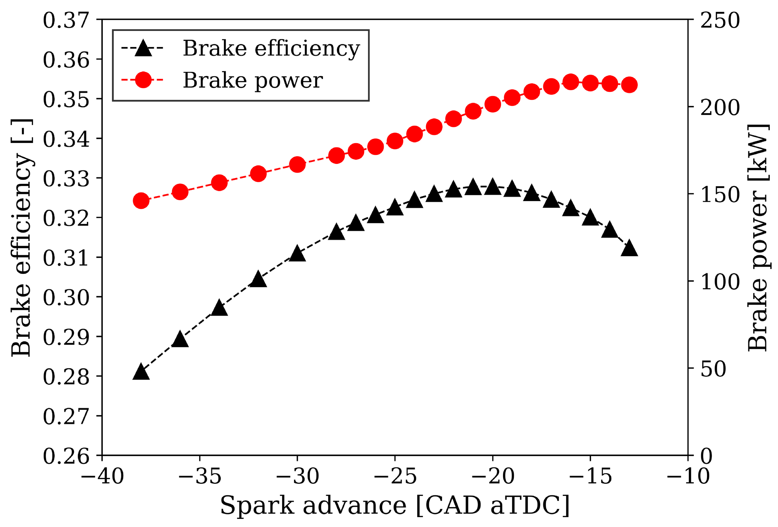
To determine the optimum SA, a sweep was performed with a completely opened WG valve. This made sure that the TC would provide the maximum boost pressure in every simulated condition. The SA was varied between −13 CAD aTDC and −38 CAD aTDC with a step of 1 CAD between −13 and −28 CAD aTDC. A step of 2 CAD was used between −28 and −38 CAD aTDC. Each simulation reached convergence before the maximum number of cycles, which was set to 200. Results in terms of brake power and brake efficiency for the SA sweep of the $\varphi =0.85$ at 1500 rpm are presented in Figure 5.

The MBP was found to be in correspondence with an SA = −16 CAD aTDC, with a value of 214.18 kW and brake efficiency equal to 32.24%. Instead, the MBE was identified at an SA = −20 CAD aTDC being equal to 32.7%, and power equal to 201 kW. The difference between the MBP and MBE is an increase of 2% in efficiency when comparing the latter with the former but connected to a reduction in power of 6%.

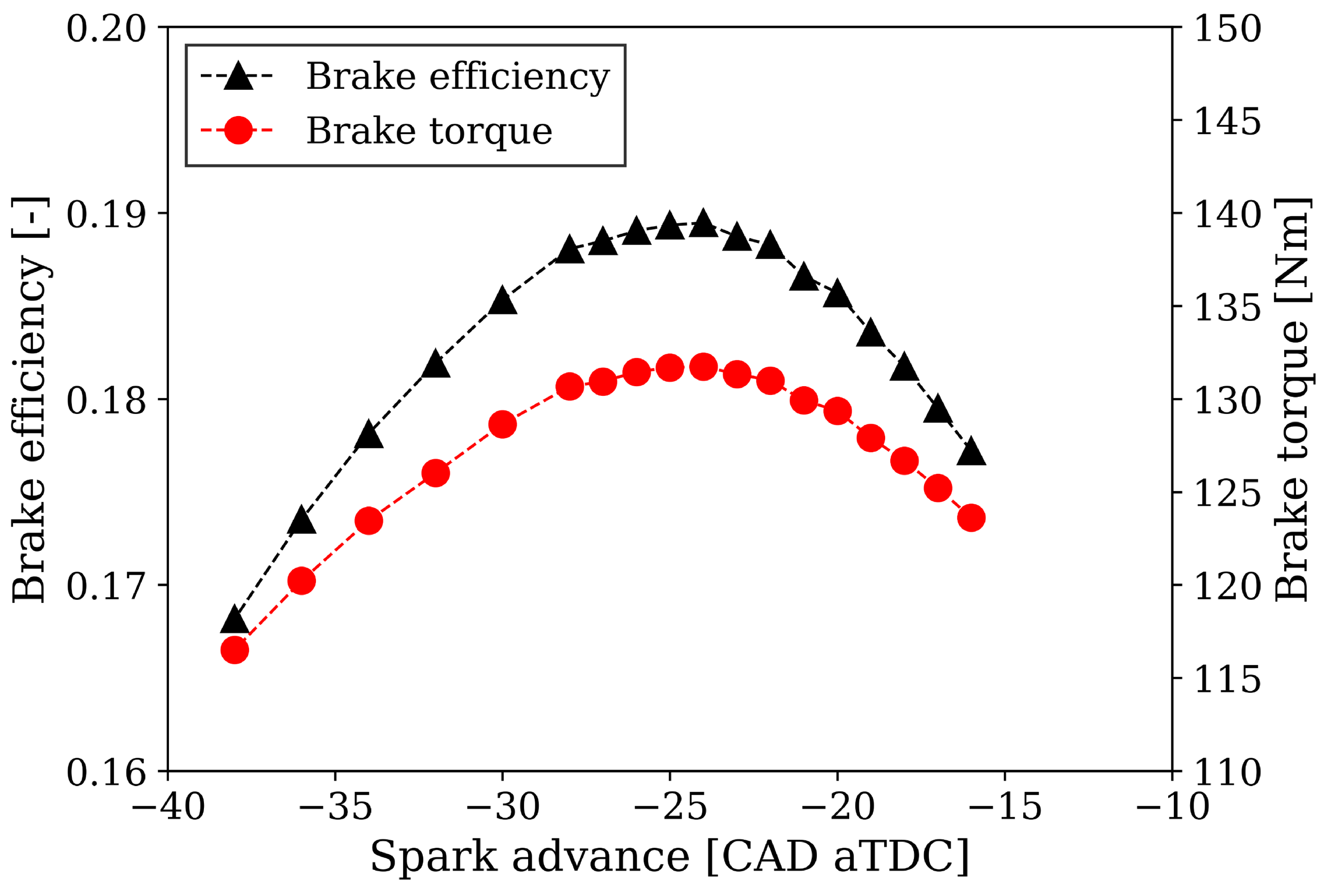
It is worth noting that these optimum SA values are not in accordance with the ones provided in the literature. As an example, in [31], a value of MBT between −20 and −25 CAD aTDC is reported at 1500 rpm for a slightly higher CR (13) and $\varphi =0.85$. However, their engine is Naturally Aspirated (NA), so it does not consider boosted conditions like in the configuration discussed in this paper. For this reason, an SA sweep was performed for a virtual NA SCE derived from the biogas engine with a CR equal to 13. In this simulation, the MBT and MBE were found both in correspondence of an SA = −24 CAD aTDC, as presented in Figure 6.

This value is in accordance with experimental results reported in [31] and further proves the capabilities of the predictive combustion model.

From the results presented in Figure 5, it is possible to say that the best operating point at $\varphi =0.85$ and 1500 rpm is in correspondence with MBP (SA = −16 CAD aTDC) due to small differences in power and efficiency with the MBE and the less retarded operating points. For these reasons, this SA was chosen to characterize the full load point of the engine. The operating conditions of the MBP are reported in

Table 4. Operative conditions characterizing the biogas-fueled engine at MBP.

Quantity	Value
Load	100	%
Engine speed	1500	rpm
Equivalence ratio	0.85
SA	−16	CAD aTDC
Wastegate valve opening	0	%
Throttle valve opening	100	%
Boost pressure	1.88	bar
Brake power	214.18	kW
Brake efficiency	32.24	%
Brake Specific Fuel Consumption (BSFC)	724.40	g/kWh
Fuel mass flow rate	155.15	kg/h

.

3.4. Partial Load Operation

Following the selection of the full load conditions, a partial load analysis was conducted to characterize the engine in a typical CHP configuration. In this setup, the engine is fueled directly with a portion of the production output of the biogas plant, which can change over time. This leads to fluctuation in the fuel flow rate that directly influences the load and power output of the engine. Partialization strategies were implemented to maintain the same equivalence ratio over a large range of partial load operating conditions. In the case studied, both the throttle valve and the WG valve were used individually or in combination to achieve the desired results. In particular, reducing the boost pressure (i.e., opening the WG valve) decreases the air intake mass flow rate. The same effect can be achieved by throttling (i.e., introducing pressure losses) with the throttle valve. In this study, partialization was implemented as follows:

• The load was varied between 100% (214.18 kW) and 30% (65.49 kW) of the full load brake paper with 10% increments;
• The WG valve was actuated with a PID controller to achieve the desired brake power until it was completely opened (i.e., the TC does not provide any boost);
• Once the WG valve was completely opened, the throttle valve was closed by a second PID controller to further reduce the air intake flow rate and obtain the target power.

For all simulated points, the SA was kept fixed at −16 CAD aTDC, as full load condition. Moreover, the equivalence ratio was set equal to $\varphi =0.85$.

Table 5. Operative conditions characterizing the biogas-fueled engine in full and partial load conditions. Engine speed = 1500 rpm, $\varphi =0.85$, SA = −16 CAD aTDC.

Load [%]	Boost Pressure [bar]	WG Valve Opening [%]	Throttle Valve Opening [%]	Fuel Mass Flow Rate [kg/h]
30	1.03	100.00	74.18	18.54
40	1.03	100.00	81.34	22.01
50	1.14	67.99	100.00	25.58
60	1.29	49.68	100.00	29.21
70	1.43	34.80	100.00	32.79
80	1.58	19.93	100.00	36.27
90	1.73	7.75	100.00	39.70
100	1.88	0.00	100.00	43.10

resumes the operating conditions simulated, reporting the opening percentages of the WG and throttle valves and the boost pressure. The throttle valve was actuated only at very low loads (30 and 40%). Instead, for higher loads, it was sufficient to act on the WG valve, thus reducing the boost pressure.

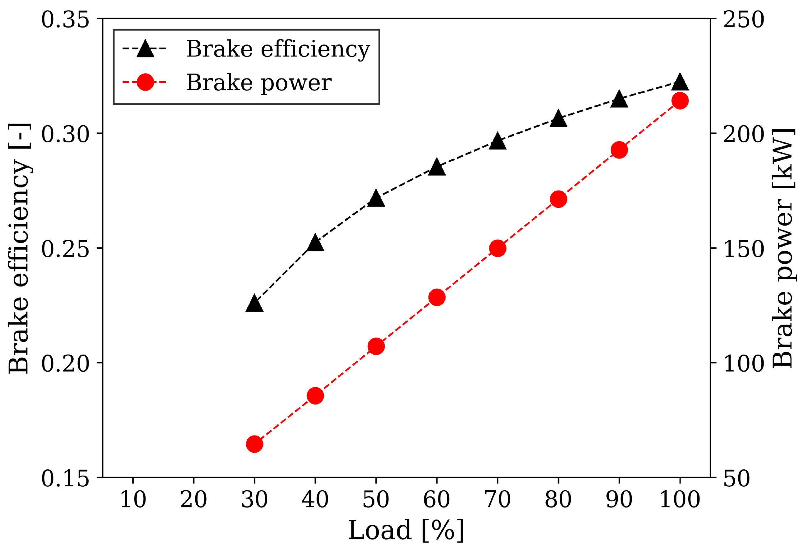
Results in terms of brake power and brake efficiency are collected in Figure 7.

As expected, brake power reduces linearly with the load due to the partialization techniques implemented. Instead, brake efficiency presents a decrease to 22% at the lowest load considered. It can also be observed that the efficiency reduction is practically linear up to a 50% load, where the throttle valve is still completely opened. A larger relative drop is observed for lower loads due to the dissipative nature of the throttle valve, which has a larger influence on efficiency. Similar trends were reported in [37].

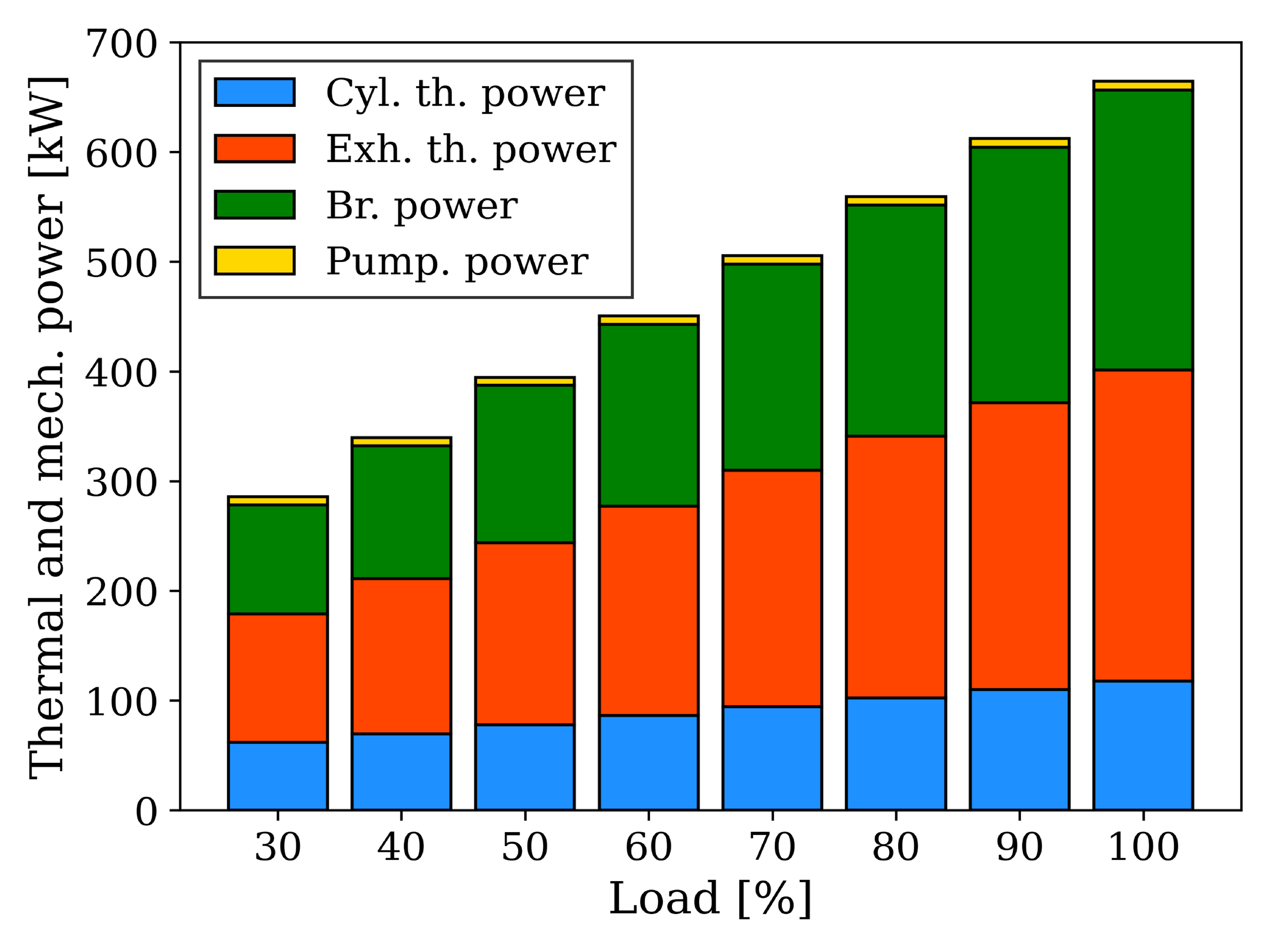
Figure 8 is a visual representation of the mechanical and thermal power flows at different loads. The sum over each bar in the graph equates to the power input, computed as the mass flow rate of fuel multiplied by its LHV. Four quantities are identified, namely pumping power (Pump. power), brake power (Br. power), thermal power exchanged with the cylinder (Cyl. th. power.), and thermal power lost in the exhaust gases (Exh. th. power). From this visualization, it is possible to appreciate the amount of thermal power that can be theoretically recovered in a CHP application of such an engine. At the lowest load, this is equal to 117.24 kW (41% of power input), while at full load, it is 283.44 kW (43% of power input). Moreover, heat can be recovered by cooling the cylinder walls to reduce the thermal stress on the engine. This accounts for 21% and 17% of the power input at the lowest and highest loads, respectively.

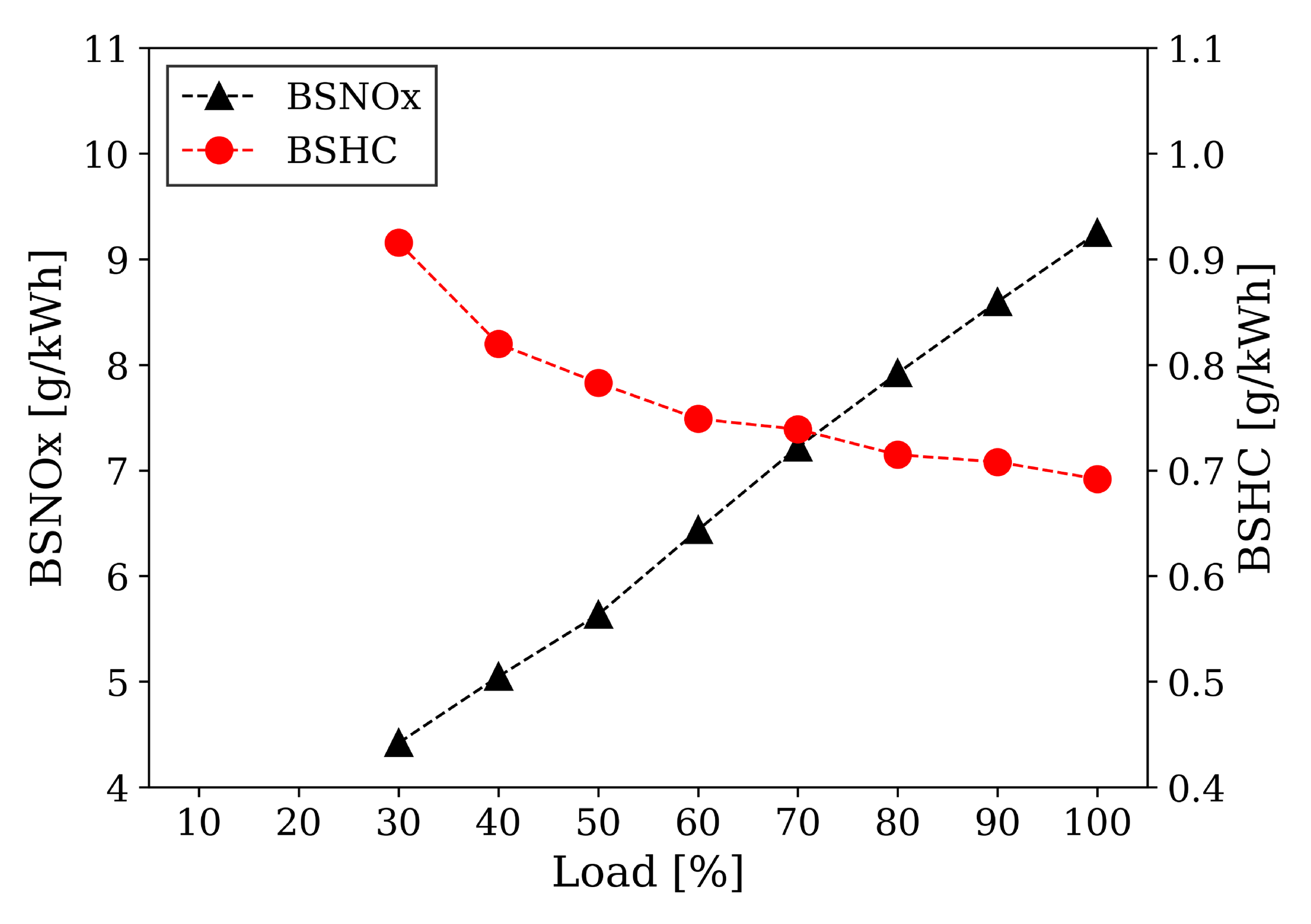
In terms of Brake Specific NO_x (BSNO_x) and Brake Specific Hydro-Carbon (BSHC) emissions, two different trends are observed, as reported in Figure 9.

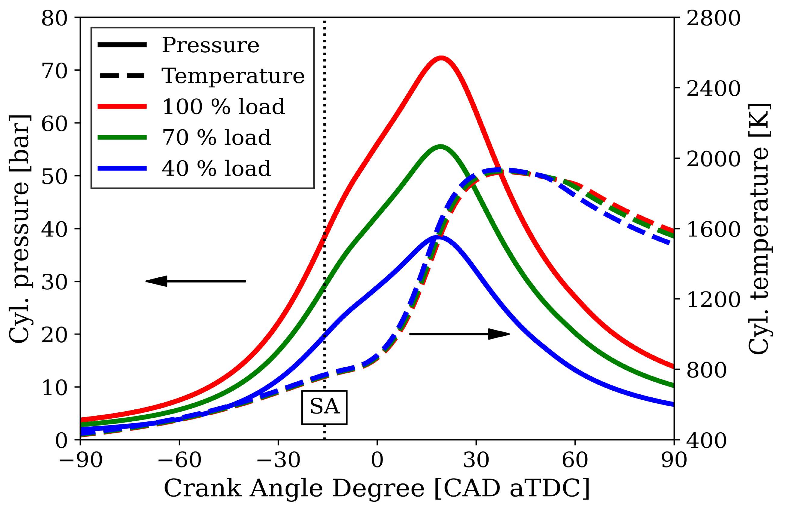
In particular, the BSNO_x increases with the load. This is expected due to higher pressures at IVC, which relates to higher trapped mass and species volumetric concentration. In-cylinder pressure and temperature trends for three loads (40, 70, and 100%) are reported in Figure 10 to provide a qualitative representation of how these quantities varied at different operating points. Computed cylinder temperatures do not vary greatly, even at low loads, due to the presence of an Inter-Cooler (IC) placed after the TC that maintains a fixed inlet temperature.

Regarding the BSHC, a negative trend with respect to load percentage is observed. The reason behind this is attributed to the higher power produced at increased loads. Indeed, results show higher absolute hydro-carbon emissions when the fuel mass flow rate is increased.

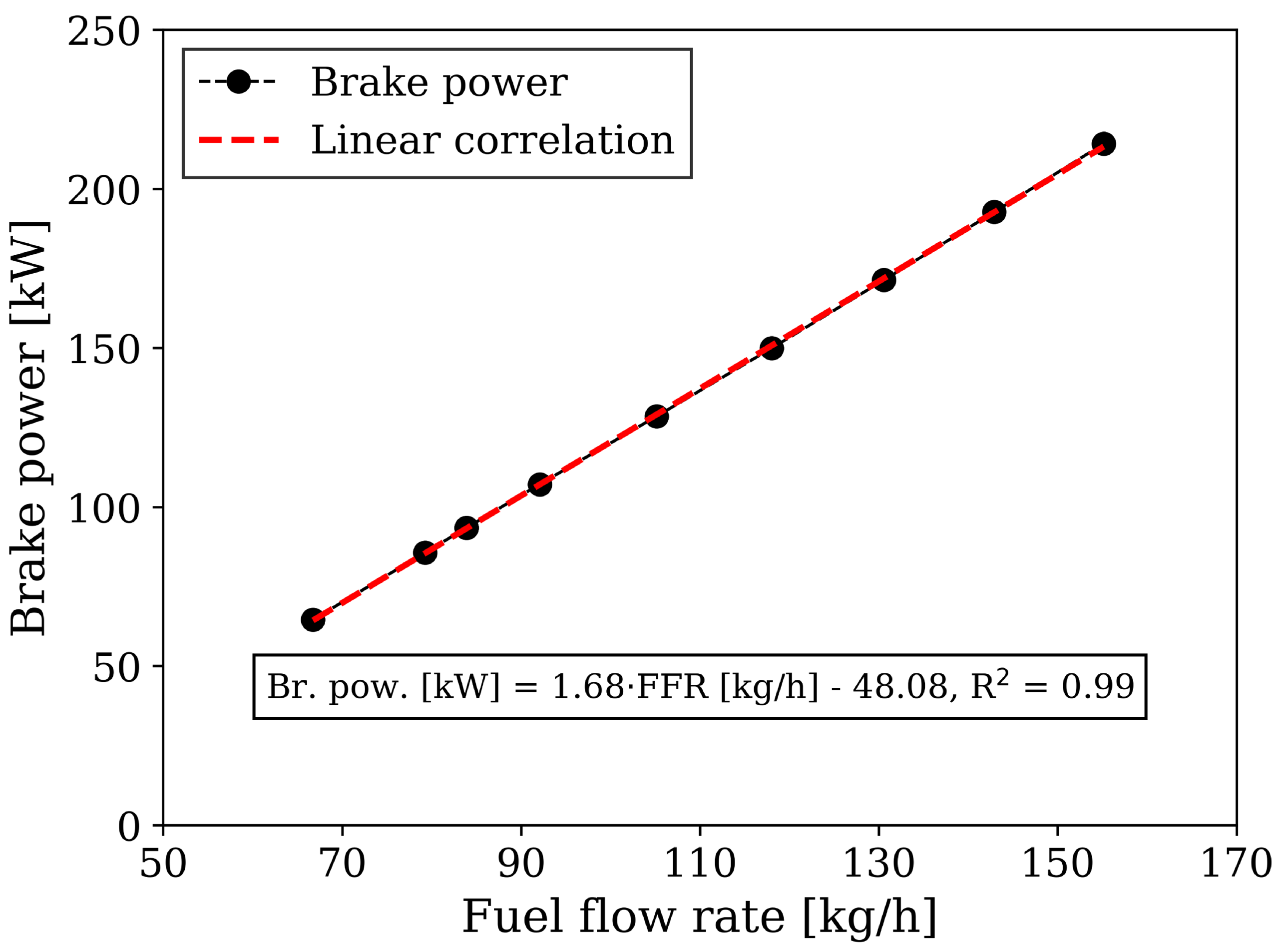
As stated previously, engine load is a direct function of the available fuel mass flow rate (FFR) in the theoretical CHP setup considered in this study. A linear correlation between the brake power ($\mathrm{Br}.\mathrm{Pow}.$) and the latter quantity can be derived, as presented in Figure 11.

Equation (4) describes the relationship between brake power and fuel mass flow rate:

$$\left\{\begin{array}{cc}\hfill & \mathrm{Br}.\mathrm{Pow}.=1.68·\mathrm{FFR}-48.08\hfill \\ \hfill & R^2=0.99\hfill \end{array}\right.$$

(4)

where $\mathrm{Br}.\mathrm{Pow}.$ is in kW and FFR is in kg/h. The linear nature of this correlation is a direct consequence of the partialization strategy employed. By initially acting on the WG valve to reduce the boost pressure, the load decreases without significantly compromising the efficiency of the engine, as presented in Figure 7. This results in an almost directly proportional reduction in brake power with respect to the fuel flow rate. This trend seems to hold even at very low load conditions (30 and 40%), where the throttle valve is also actuated and a greater decrease in efficiency is noticeable. A possible explanation for this is that at lower power outputs the reduction in efficiency does not result in a large variation in fuel flow rate. This relationship can be used in simulations and optimizations of complete production plants in a so-called “black-box” approach [38,39]. In such analyses, the engine is treated as a component of the plant and is characterized only by a simple equation, like the one reported in Equation (4). This enables the use of results obtained by complete and thorough engine simulations without increasing the computational burden of the plant’s optimization software. One example of such simulation and optimization application can be found in the work by Nava [15].

4. Comparison Between CNG and Biogas Operations

This Section presents a comparison between the full load conditions of the CNG engine and the biogas-converted one. The characteristics of the operative conditions being compared are reported in

Table 6. Comparison between CNG and biogas-fueled engine at 1500 rpm, full load conditions.

Quantity	CNG Engine	Biogas Engine
Load	100		%
Engine speed	1500		rpm
Eq. ratio	1.00	0.85
Boost pressure	1.98	1.87	bar
Brake power	295.74	214.18	kW
Brake efficiency	33.65	32.24	%
BSFC	226.36	724.40	g/kWh
Fuel mass flow rate	70.56	155.15	kg/h
SA	−5	−16	CAD aTDC
${\theta }_{10}$	11	6	CAD aTDC
${\theta }_{50}$	20	20	CAD aTDC
${\theta }_{90}$	32	44	CAD aTDC
${\theta }_{10–90}$	21	38	CAD

.

It is important to note that the engines have different equivalence ratios. However, lean combustion was chosen for biogas engines as it is beneficial for brake efficiency and allows for stable operations, as discussed in Section 3.3.

In terms of brake power, a reduction of 33% is observed for the biogas configuration compared to the CNG engine. The loss in power is expected due to the nature of the fuel. In fact, in these simulations, the mass fraction of CH₄ contained in the biogas stream is 31%. This means that the actual CH₄ mass flow rate is 48.09 kg/h, which equates to ca. 70% of the fuel flow rate of the CNG engine. As a result, the lower quantity of CH₄ results in a reduction in power output of more or less the same percentage. The conversion of the engine to biogas also affects the brake efficiency, reducing it by 4%. 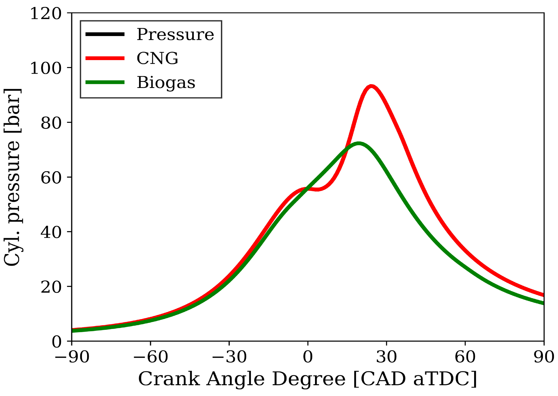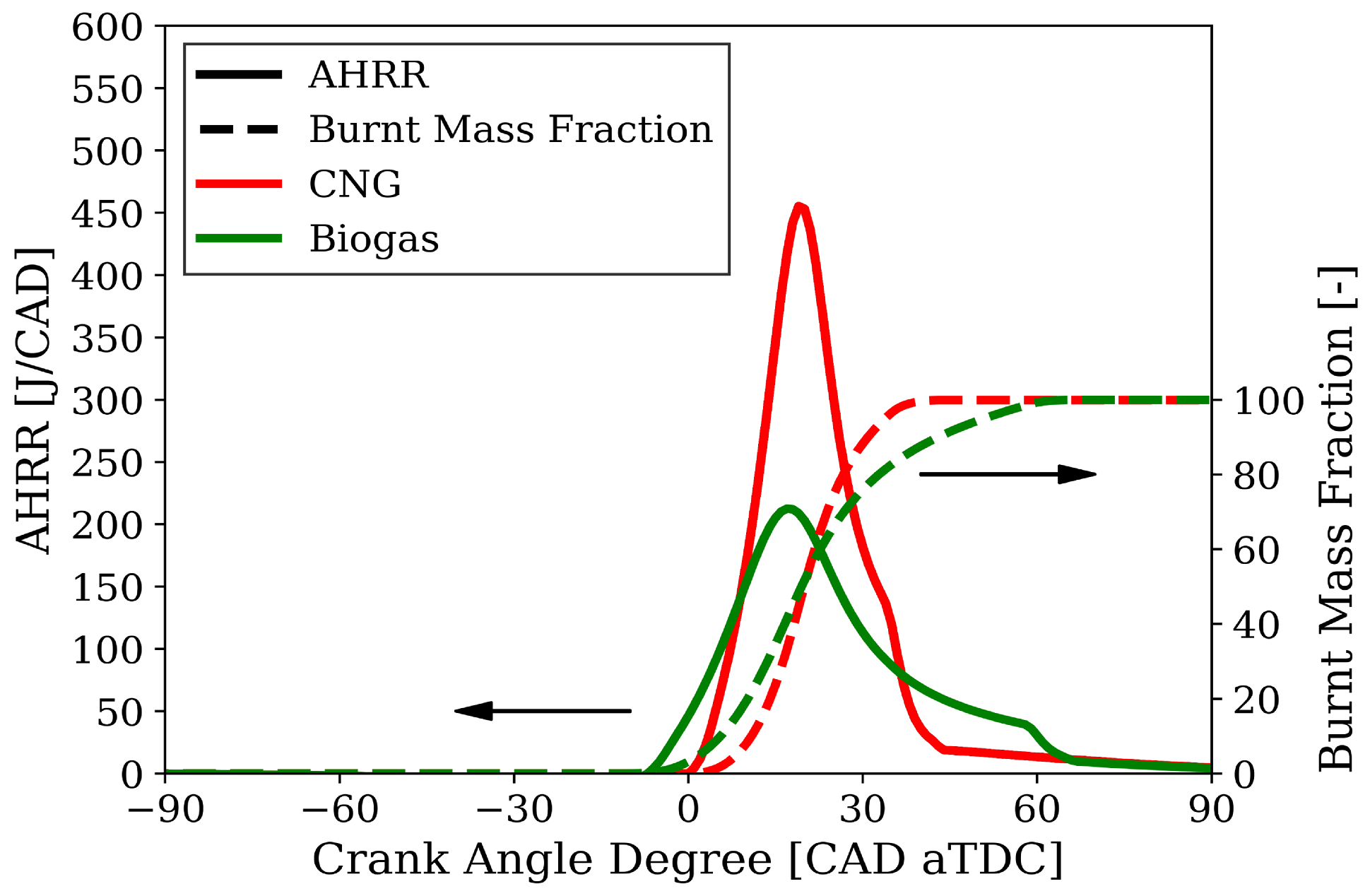This can be explained by considering the differences between the combustion characteristics of the fuels, as discussed in Section 3.2. Indeed, the lower laminar flame speed of biogas results in slower combustion, thus moving apart from the isochoric combustion of the ideal Otto cycle. This is evident by observing the in-cylinder pressure, Burnt Mass Fraction (BMF) and AHRR trends reported in Figure 12 and Figure 13, respectively. Figure 12 shows that completely different pressure trends characterize the combustion and expansion phases in the two configurations, despite presenting similar compression curves. These differences can be explained by looking at Figure 13. A much steeper rise in BMF is reported for the CNG combustion with respect to biogas. Combustion duration increases from ${\theta }_{10–90,\mathit{CNG}}=21$ CAD of the CNG configuration to ${\theta }_{10–90,\mathit{bio}}=38$ CAD for biogas. Additionally, the SA had to be reduced considerably to obtain a similar pressure peak position. This is noticed by looking at the values of ${\theta }_{10}$, ${\theta }_{50}$, ${\theta }_{90}$ that characterize the combustion process collected in Table 6. Although both configurations show the same ${\theta }_{50}$, the biogas one is characterized by a delayed ${\theta }_{10–90}$, and also an increased combustion duration between SA and ${\theta }_{10}$. This is due to the lower concentration of methane in the biogas-fueled engine that reduces combustion speed. The effect of high CO₂ content on LHV and burning rate can be further observed in the AHRR comparison reported in Figure 13. A broader trend with a lower peak value characterizes the biogas configuration, whereas CNG presents a sharper increase in AHRR with a much higher maximum value. This is the direct result of the slower combustion and the reduced LHV of biogas. Combustion efficiency is close to 100% for both cases.

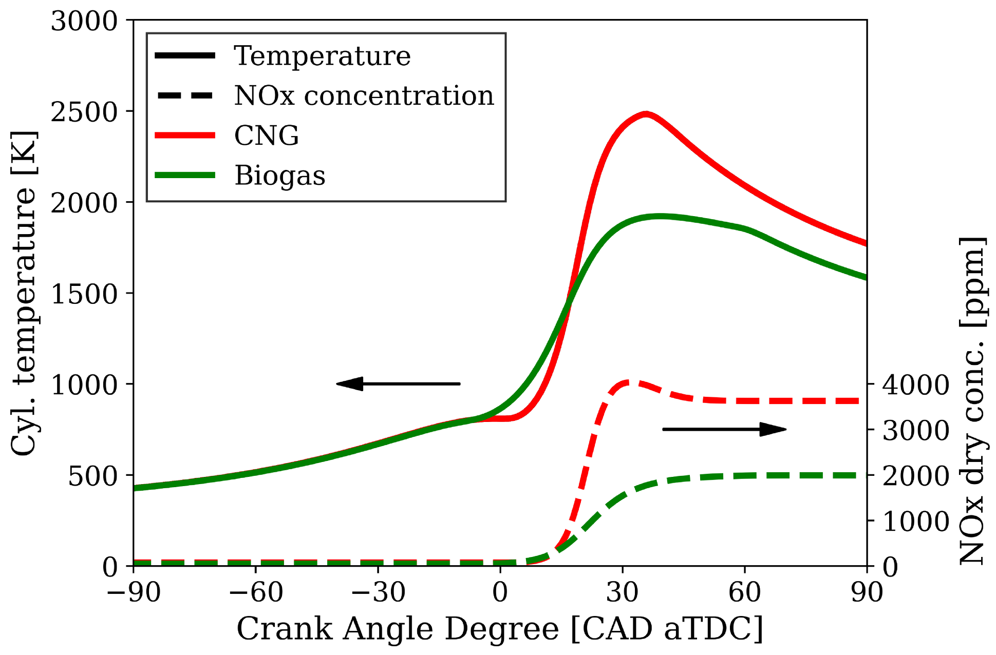
In addition, the presence of a high quantity of CO₂ in biogas greatly affects the in-cylinder temperature trends as presented in Figure 14.

Indeed, the higher heat capacity of the fresh mixture in the biogas engine allows for dampening the temperature rise and so the maximum temperature reached, which is 1921 K. Instead, in the CNG configuration, a peak temperature of 2482 K is observed. As a result, the production of NO_x lowers to almost half of the dry molar concentration when comparing the CNG engine (3626 ppm) to the biogas one (1990 ppm). However, the BSNO_x in the two configurations is similar due to the power reduction in the biogas engine. The CNG engine presents a BSNO_x of 11.32 g/kWh, whereas the biogas one is 9.25 g/kWh. It is worth noting that both the analyzed configurations, NO_x emissions would require an after-treatment system to obtain acceptable emission levels compliant with the local regulation. BSHC emissions for the CNG engine are equal to 0.32 g/kWh, compared to 0.69 g/kWh for the biogas configuration.

5. Conclusions

Biogas is expected to have an increasing role in reducing CO₂ emissions to reach the GHG reduction targets. Several studies have explored the effects on performance of using this fuel with varying CO₂ content in LD SI engines. However, there is a scarcity of data relative to biogas-powered HD SI engines in the literature. This paper aims to numerically assess the feasibility and performance implications derived from the conversion to biogas of a CNG-fueled HD SI engine. The study can be summarized as follows:

• A commercial HD SI CNG engine was modeled in a 1D software. The model was validated against experimental data. The baseline engine configuration was later modified to be fueled with biogas. In particular, only the fuel injection system was changed to represent a single Venturi mixer placed upstream of the compressor.
• Specific laminar flame speed corrections were introduced to account for biogas combustion characteristics. All other combustion sub-models were maintained the same as for the CNG engine.
• SA sweeps were performed at lean and stoichiometric conditions and 1500 rpm. Stoichiometric conditions showed unstable operations due to the TC system. Lean conditions were chosen and further investigated. A partial load analysis was carried out starting from the MBP operating point by actuating the WG and throttle valves.
• The conversion to biogas showed a reduction in both power (33%) and efficiency (4%) at full load conditions and 1500 rpm with respect to the CNG one.
• The results prove the possibility and the expected changes in performance resulting from the conversion to biogas of a CNG HD SI engine. Moreover, the results from the part load analysis can be used in techno-economic analysis of biogas production plants with a biogas-fueled ICE in CHP configuration.
• The presented methodology can be applied to investigate possible strategies to reduce performance losses derived from the fuel conversion presented in the study. As an example, increasing the compression ratio or introducing a different TC system are solutions expected to shrink the gap between the CNG and biogas engines.