

Inherent Risk Analysis of Power Supply Management: Case of Belize’s System Operator and Third-Party Actors


Abstract
1. Introduction
2. Literature Review
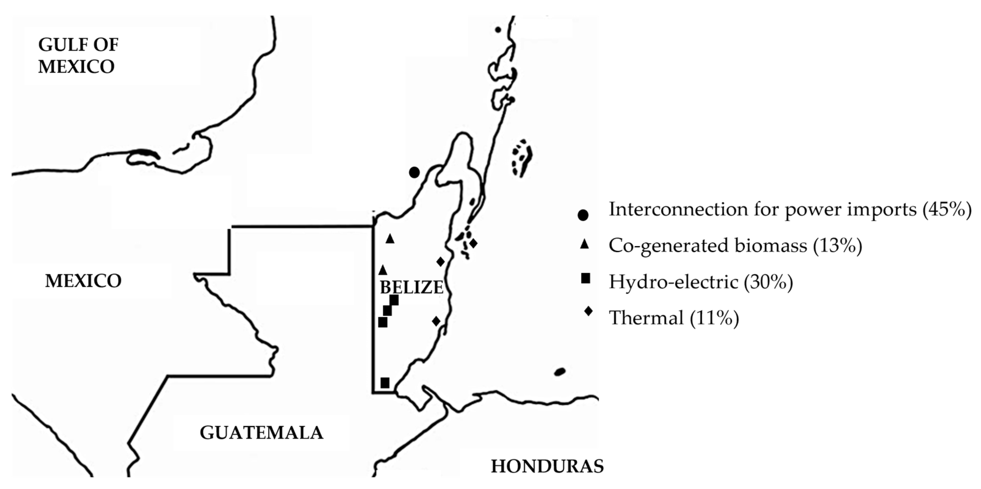
2.1. Background of the Case Study
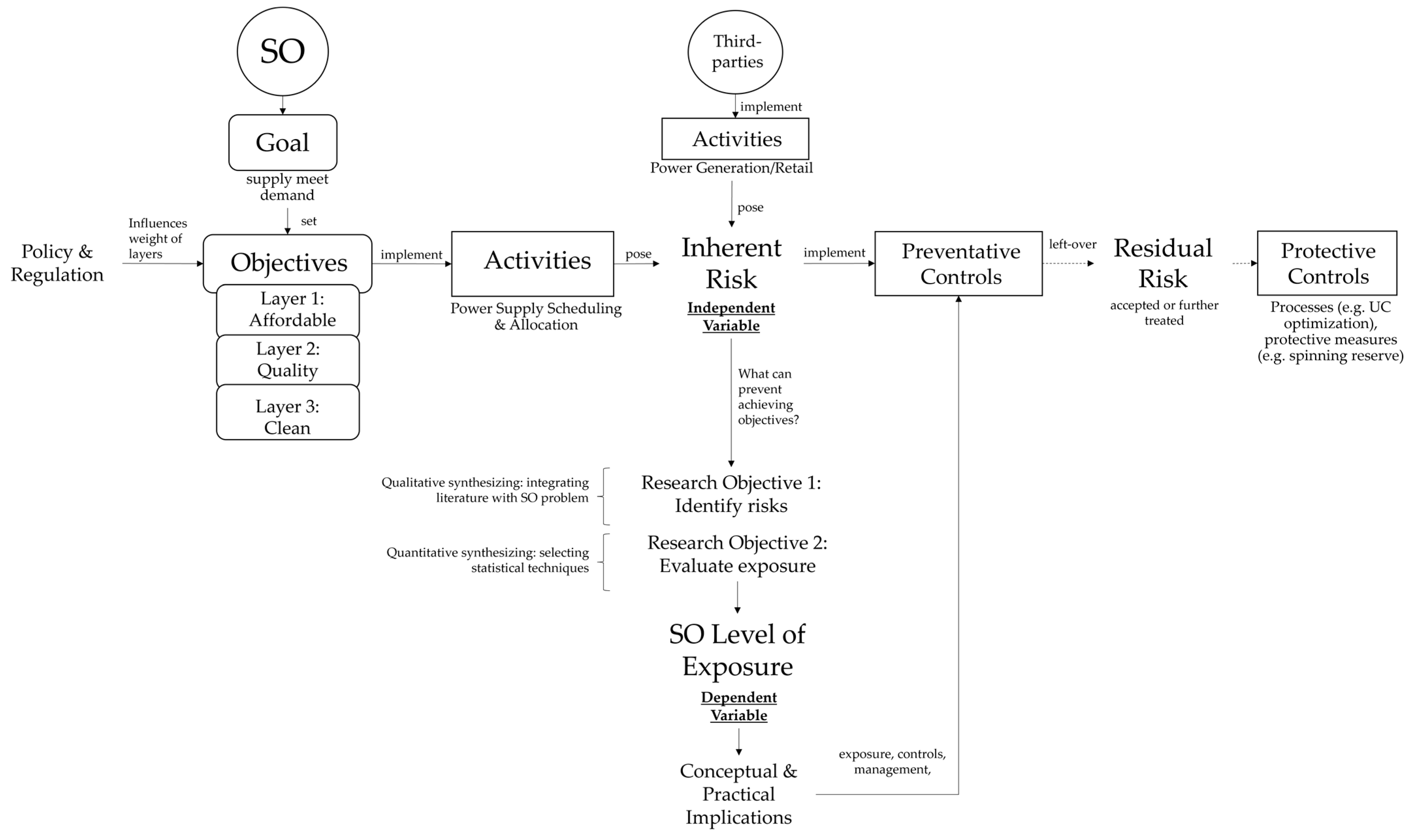
2.2. Residual Versus Inherent Risk Contextualized for the Operations of an SO
- The most widely discussed is to schedule and allocate at the lowest possible cost and maintain the affordability of power for consumers. The energy industry uses the term ‘merit order’ [12] to describe the sequence by which power supply is allocated and scheduled on an economic basis like lowest cost.
- Scheduling and allocating to achieve high power quality [3]. High power quality means the combined supply remains steady and within prescribed voltage, frequency, and waveform standards [20]. By maintaining high power quality, SOs also ascertain compatibility with the electrical devices of consumers. Poor power quality can cause devices to malfunction.
- The most novel is to prioritize renewable and clean energy sources. SOs incorporate climate goals to reduce sources, like fossil fuels and coal, which contribute to greenhouse gasses (GHGs) or other major pollutants. Notably, variable renewable energy (VRE) is prioritized in the merit order, having zero marginal cost [21].
2.3. Conceptual Framework
3. Materials and Methods
3.1. Data
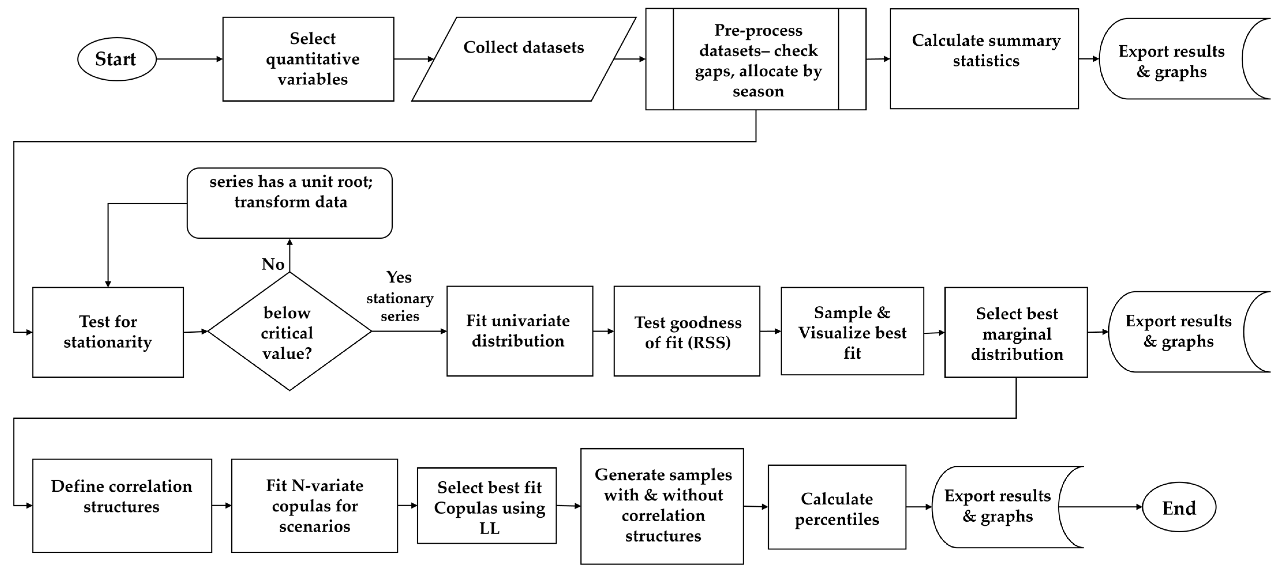
3.2. Study Design
3.2.1. Objective 1—Qualitative Synthesis of Inherent Risk Factors
3.2.2. Object 2—Quantitative Assessment of Exposure Level
3.3. Description of Statistical Analyses Applied in This Study
3.3.1. Summary Statistics and Marginal Distribution
3.3.2. Joint Distributions Based on Copula Technique
4. Results and Discussion
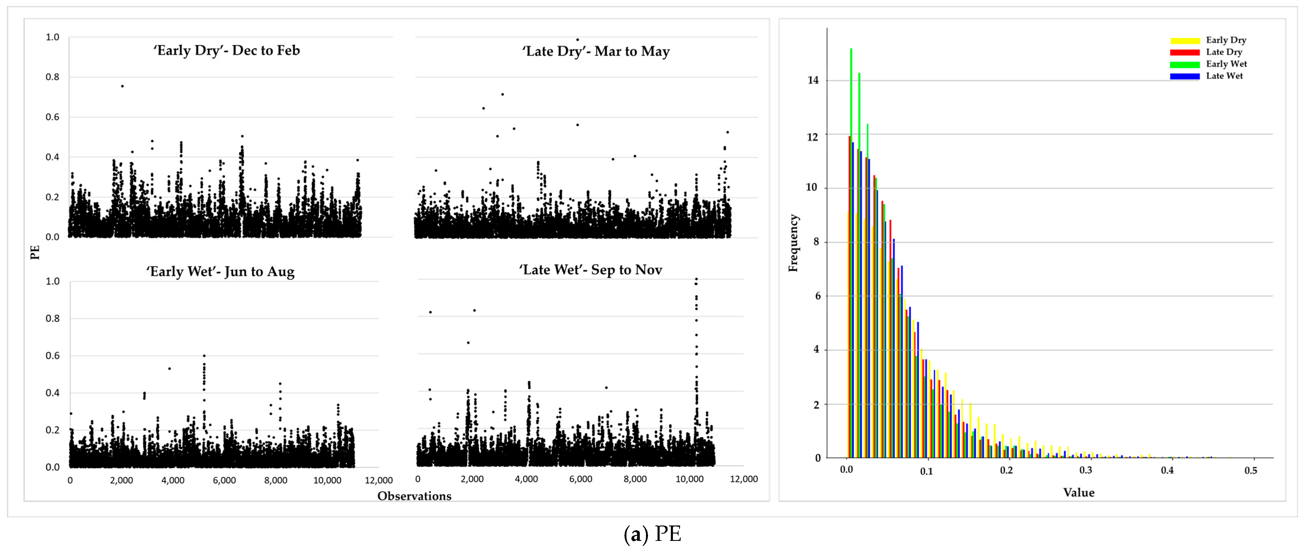
4.1. Summary Statistics
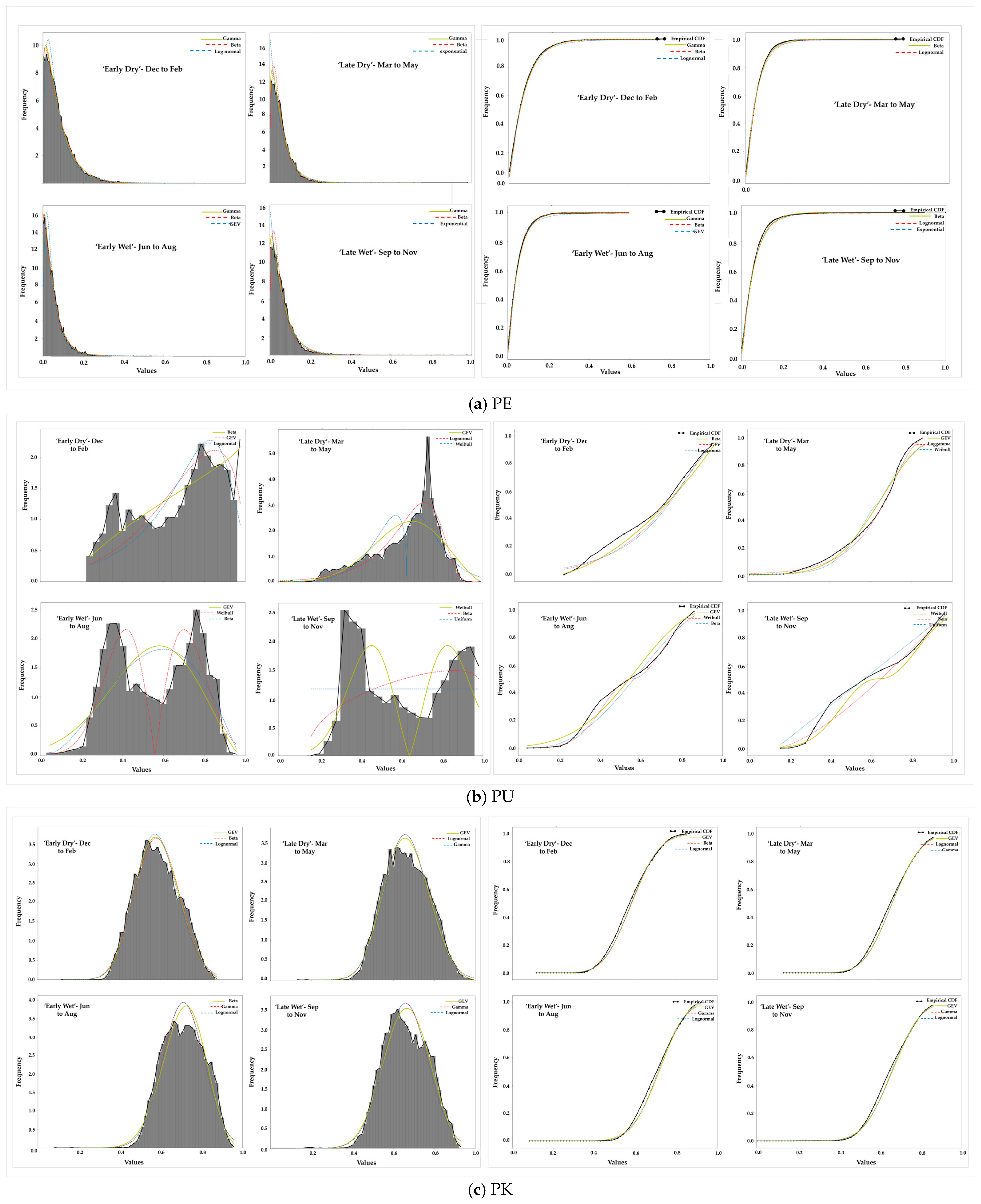
4.2. Marginal Distributions—Parameter Estimation and Fitting
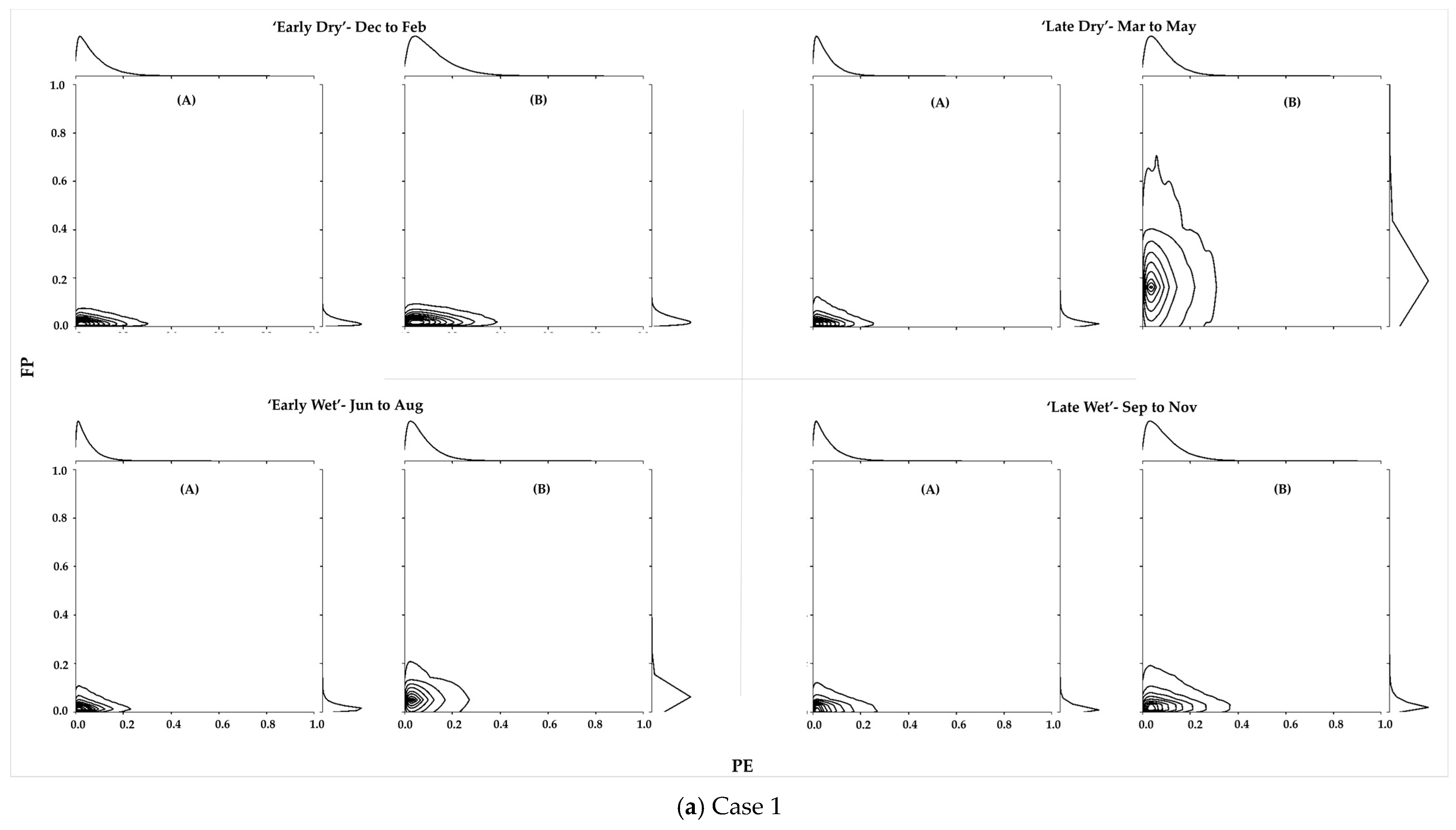
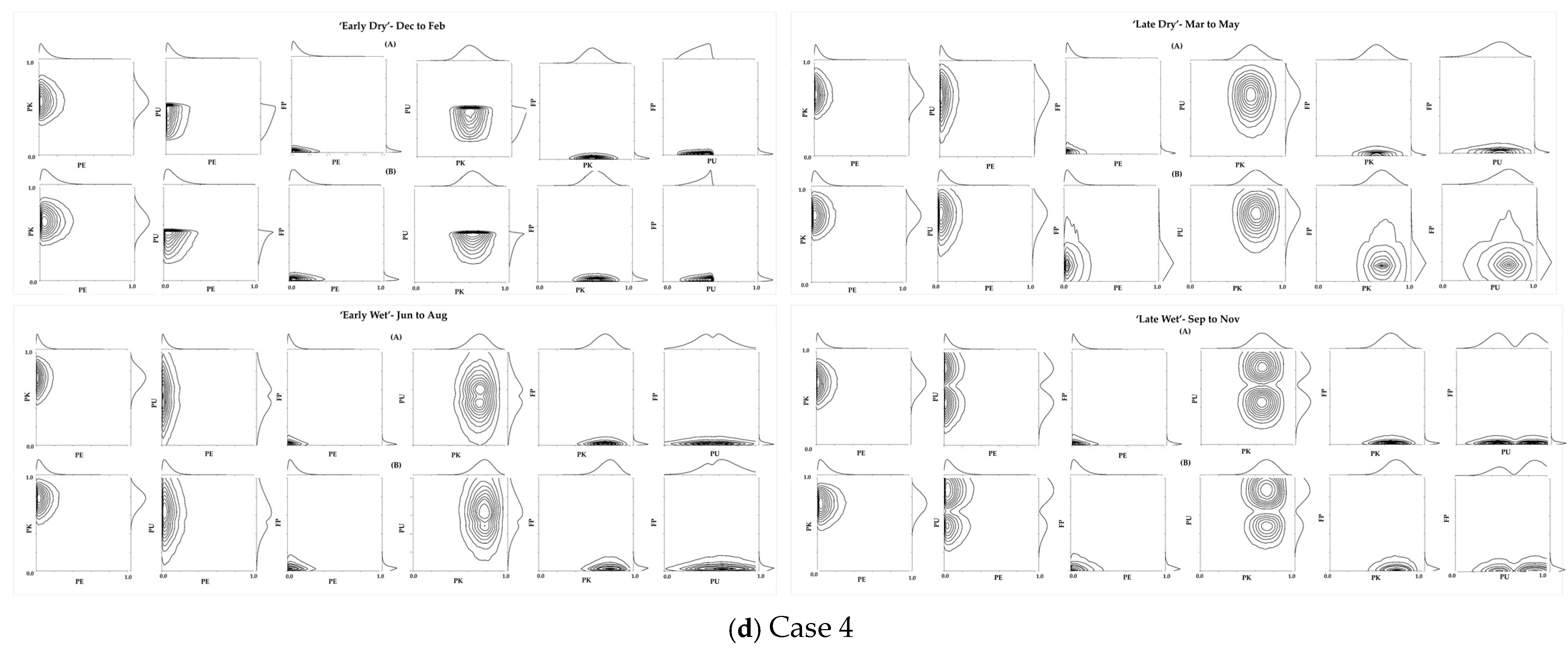
4.3. Joint Distribution Parameter Estimation and Fitting
4.4. Relative Levels of Exposure per Season and Inferences on Preventative Controls
5. Conclusions
Author Contributions
Funding
Data Availability Statement
Acknowledgments
Conflicts of Interest
Appendix A

| Distribution | Probability Density Function | Parameter |
|---|---|---|
| normal | μ—mean σ—standard deviation | |
| exponential | λ—rate parameter | |
| Pareto | xm—minimum possible value of x α—shape parameter/tail index | |
| Weibull | k—shape parameter λ—scale of distribution | |
| t | ν—degrees of freedom Γ—gamma function | |
| GEV | —shape parameter s—location parameter | |
| gamma | α,β—shape parameters Γ—gamma function | |
| log-normal | μ—natural log mean σ—natural log standard deviation | |
| beta | α,β—shape parameters B—normalization constant | |
| uniform | a,b—minimum and maximum bounds | |
| log-gamma | α—shape parameters λ—scale of distribution Γ—gamma function |
| (a) PE | |||
| Season | Distribution | RSS | Rank |
| Early Dry | normal | 174.135 | 9 |
| exponential | 24.234 | 3 | |
| Pareto | 24.234 | 3 | |
| Weibull | 125.247 | 8 | |
| t | 119.414 | 7 | |
| GEV | 38.240 | 6 | |
| gamma | 3.475 | 2 | |
| log-normal | 25.570 | 5 | |
| beta | 2.831 | 1 | |
| uniform | 664.120 | 11 | |
| log-gamma | 178.426 | 10 | |
| Late Dry | normal | 299.378 | 9 |
| exponential | 71.087 | 3 | |
| Pareto | 71.087 | 3 | |
| Weibull | 213.689 | 7 | |
| t | 203.947 | 6 | |
| GEV | 81.456 | 5 | |
| gamma | 697.393 | 10 | |
| log-normal | 61.608 | 2 | |
| beta | 16.399 | 1 | |
| uniform | 1447.070 | 11 | |
| log-gamma | 296.963 | 8 | |
| Early Wet | normal | 492.381 | 9 |
| exponential | 29.889 | 3 | |
| Pareto | 29.889 | 3 | |
| Weibull | 347.407 | 8 | |
| t | 323.893 | 7 | |
| GEV | 108.585 | 6 | |
| gamma | 6.221 | 2 | |
| log-normal | 66.800 | 5 | |
| beta | 6.095 | 1 | |
| uniform | 1681.720 | 11 | |
| log-gamma | 503.463 | 10 | |
| Late Wet | normal | 327.835 | 8 |
| exponential | 40.318 | 2 | |
| Pareto | 42.010 | 3 | |
| Weibull | 215.910 | 7 | |
| t | 190.403 | 6 | |
| GEV | 68.808 | 5 | |
| gamma | 531.113 | 10 | |
| log-normal | 47.286 | 4 | |
| beta | 11.206 | 1 | |
| uniform | 1227.130 | 11 | |
| log-gamma | 354.224 | 9 | |
| (b) PU | |||
| Season | Distribution | RSS | Rank |
| Early Dry | normal | 9.467 | 6 |
| exponential | 23.191 | 10 | |
| Pareto | 23.191 | 10 | |
| Weibull | 8.410 | 5 | |
| t | 9.467 | 7 | |
| GEV | 4.385 | 2 | |
| gamma | 10.011 | 9 | |
| log-normal | 9.467 | 8 | |
| beta | 2.485 | 1 | |
| uniform | 6.220 | 4 | |
| log-gamma | 5.590 | 3 | |
| Late Dry | normal | 26.650 | 6 |
| exponential | 96.983 | 10 | |
| Pareto | 96.983 | 10 | |
| Weibull | 24.676 | 3 | |
| t | 25.688 | 4 | |
| GEV | 21.623 | 2 | |
| gamma | 29.540 | 7 | |
| log-normal | 26.471 | 5 | |
| beta | 37.028 | 8 | |
| uniform | 67.458 | 9 | |
| log-gamma | 9.888 | 1 | |
| Early Wet | normal | 13.158 | 6 |
| exponential | 32.313 | 10 | |
| Pareto | 32.313 | 10 | |
| Weibull | 5.434 | 1 | |
| t | 13.158 | 8 | |
| GEV | 11.274 | 3 | |
| gamma | 13.139 | 4 | |
| log-normal | 13.158 | 6 | |
| beta | 9.351 | 2 | |
| uniform | 17.440 | 9 | |
| log-gamma | 13.145 | 5 | |
| Late Wet | normal | 14.676 | 8 |
| exponential | 21.628 | 10 | |
| Pareto | 21.628 | 10 | |
| Weibull | 7.861 | 1 | |
| t | 14.676 | 8 | |
| GEV | 13.691 | 5 | |
| gamma | 14.610 | 7 | |
| log-normal | 13.383 | 4 | |
| beta | 9.031 | 2 | |
| uniform | 10.495 | 3 | |
| log-gamma | 14.589 | 6 | |
| (c) PK | |||
| Season | Distribution | RSS | Rank |
| Early Dry | normal | 3.429 | 6 |
| exponential | 144.361 | 10 | |
| Pareto | 144.361 | 10 | |
| Weibull | 10.965 | 8 | |
| t | 3.429 | 7 | |
| GEV | 2.040 | 1 | |
| gamma | 2.586 | 4 | |
| log-normal | 2.581 | 3 | |
| beta | 2.331 | 2 | |
| uniform | 92.019 | 9 | |
| log-gamma | 3.389 | 5 | |
| Late Dry | normal | 3.384 | 5 |
| exponential | 138.269 | 10 | |
| Pareto | 138.269 | 10 | |
| Weibull | 5.557 | 8 | |
| t | 3.384 | 6 | |
| GEV | 2.100 | 1 | |
| gamma | 3.019 | 3 | |
| log-normal | 2.997 | 2 | |
| beta | 4.235 | 7 | |
| uniform | 94.236 | 9 | |
| log-gamma | 3.321 | 4 | |
| Early Wet | normal | 5.373 | 4 |
| exponential | 161.130 | 10 | |
| Pareto | 161.130 | 10 | |
| Weibull | 7.091 | 7 | |
| t | 5.373 | 5 | |
| GEV | 125.856 | 9 | |
| gamma | 5.299 | 2 | |
| log-normal | 5.373 | 3 | |
| beta | 4.894 | 1 | |
| uniform | 111.461 | 8 | |
| log-gamma | 5.509 | 6 | |
| Late Wet | normal | 4.556 | 5 |
| exponential | 145.056 | 10 | |
| Pareto | 145.056 | 10 | |
| Weibull | 6.535 | 8 | |
| t | 4.556 | 4 | |
| GEV | 3.657 | 1 | |
| gamma | 4.315 | 2 | |
| log-normal | 4.449 | 3 | |
| beta | 4.705 | 6 | |
| uniform | 100.576 | 9 | |
| log-gamma | 4.866 | 7 | |
| (d) FP | |||
| Season | Distribution | RSS | Rank |
| Early Dry | normal | 4275.100 | 7 |
| exponential | 563.132 | 1 | |
| Pareto | 775.352 | 3 | |
| Weibull | 2180.030 | 6 | |
| t | 1583.700 | 5 | |
| GEV | 965.400 | 4 | |
| gamma | 5923.220 | 9 | |
| log-normal | 11,555.600 | 11 | |
| beta | 593.196 | 2 | |
| uniform | 11,349.300 | 10 | |
| log-gamma | 4491.330 | 8 | |
| Late Dry | normal | 5035.380 | 7 |
| exponential | 555.753 | 1 | |
| Pareto | 855.044 | 3 | |
| Weibull | 3050.850 | 6 | |
| t | 1488.620 | 5 | |
| GEV | 836.784 | 2 | |
| gamma | 6770.940 | 9 | |
| log-normal | 11,551.600 | 10 | |
| beta | 1259.270 | 4 | |
| uniform | 11,904.600 | 11 | |
| log-gamma | 5636.840 | 8 | |
| Early Wet | normal | 4648.500 | 7 |
| exponential | 1331.130 | 4 | |
| Pareto | 1781.760 | 5 | |
| Weibull | 3169.760 | 6 | |
| t | 857.826 | 3 | |
| GEV | 452.987 | 1 | |
| gamma | 8813.020 | 9 | |
| log-normal | 12,178.800 | 11 | |
| beta | 736.449 | 2 | |
| uniform | 11,979.900 | 10 | |
| log-gamma | 5163.200 | 8 | |
| Late Wet | normal | 5262.680 | 7 |
| exponential | 713.711 | 2 | |
| Pareto | 1065.730 | 4 | |
| Weibull | 1895.200 | 6 | |
| t | 1192.070 | 5 | |
| GEV | 687.460 | 1 | |
| gamma | 7716.980 | 9 | |
| log-normal | 11,686.800 | 10 | |
| beta | 762.518 | 3 | |
| uniform | 12,064.100 | 11 | |
| log-gamma | 5648.630 | 8 | |
| Case | Variables | Season | LL | |
|---|---|---|---|---|
| Gaussian | t | |||
| 1 | [PE, FP] | Early dry | 0.4012 | −0.3928 |
| Late dry | 0.7780 | 0.8374 | ||
| Early wet | 0.3306 | 1.5575 | ||
| Late wet | 2.4448 | 3.0894 | ||
| 2 | [PU, PK] | Early dry | 0.0489 | −0.8444 |
| Late dry | 0.0616 | −0.7765 | ||
| Early wet | 0.1490 | 1.4114 | ||
| Late wet | −0.0050 | −0.1373 | ||
| 3 | [PK, PU, FP] | Early dry | 5.7091 | 5.1105 |
| Late dry | 1.1653 | −0.6835 | ||
| Early wet | 0.8230 | 1.2862 | ||
| Late wet | 0.2672 | −2.4446 | ||
| 4 | All | Early dry | 6.8772 | 3.4665 |
| Late dry | 3.6390 | −1.3443 | ||
| Early wet | 1.5505 | 2.7388 | ||
| Late wet | 3.5941 | 1.9977 | ||
References
- Hong, Y.Y.; Apolinario, G.F.D.; Lu, T.K.; Chu, C.C. Chance-constrained unit commitment with energy storage systems in electric power systems. Energy Rep. 2022, 8, 1067–1090. [Google Scholar] [CrossRef]
- Kadir, K.; Mehdi Salehi Dezfouli, M.; Gabrielli, L.; Greta Ruggeri, A.; Scarpa, M. Roadmap to a Sustainable Energy System: Is Uncertainty a Major Barrier to Investments for Building Energy Retrofit Projects in Wide City Compartments? Energies 2023, 16, 4261. [Google Scholar] [CrossRef]
- Tehero, R.; Aka, E.B.; Çokgezen, M. Drivers of the quality of electricity supply. Int. J. Energy Econ. Policy 2020, 10, 183–195. [Google Scholar] [CrossRef]
- Wang, Y.; Rousis, A.O.; Strbac, G. On microgrids and resilience: A comprehensive review on modeling and operational strategies. Renew. Sustain. Energy Rev. 2020, 134, 110313. [Google Scholar] [CrossRef]
- Huang, J.; Tan, Q.; Zhang, T.; Wang, S. Energy-water nexus in low-carbon electric power systems: A simulation-based inexact optimization model. J. Environ. Manag. 2023, 338, 117744. [Google Scholar] [CrossRef]
- Zhong, W.; Guo, J.; Chen, L.; Zhou, J.; Zhang, J.; Wang, D. Future hydropower generation prediction of large-scale reservoirs in the upper Yangtze River basin under climate change. J. Hydrol. 2020, 588, 125013. [Google Scholar] [CrossRef]
- Qiu, H.; Chen, L.; Zhou, J.; He, Z.; Zhang, H. Risk analysis of water supply-hydropower generation-environment nexus in the cascade reservoir operation. J. Clean. Prod. 2021, 283, 124239. [Google Scholar] [CrossRef]
- Chen, L.; Huang, K.; Zhou, J.; Duan, H.F.; Zhang, J.; Wang, D.; Qiu, H. Multiple-risk assessment of water supply, hydropower and environment nexus in the water resources system. J. Clean. Prod. 2020, 268, 122057. [Google Scholar] [CrossRef]
- Miller, T.C.; Cipriano, M.; Ramsay, R.J. Do auditors assess inherent risk as if there are no controls? Manag. Audit. J. 2012, 27, 448–461. [Google Scholar] [CrossRef]
- Gupta, C.; Bhatia, S. The inherent risk of climate change becoming a hindrance in a business supply chain. In Contemporary Studies of Risks in Emerging Technology, Part A (Emerald Studies in Finance, Insurance, and Risk Management); Emerald Publishing Limited: Leeds, UK, 2023; pp. 127–137. [Google Scholar] [CrossRef]
- IRCG. Involving Stakeholders in the Risk Governance Process; EPFL International Risk Governance Center: Lausanne, Switzerland, 2020; p. 8. [Google Scholar] [CrossRef]
- Buraimoh, E.; Park, H. A Unit Commitment Model Considering Feasibility of Operating Reserves under Stochastic Optimization Framework. Energies 2022, 15, 6221. [Google Scholar] [CrossRef]
- Bachev, H. Risk Management in the Agri-Food Sector. Contemp. Econ. 2013, 7, 45–62. [Google Scholar] [CrossRef]
- Zambrano, A. An Overview of Application of Optimization Models Under Uncertainty to the Unit Commitment Problem. arXiv 2022, arXiv:2203.16883v1. [Google Scholar]
- Yang, N.; Dong, Z.; Wu, L.; Zhang, L.; Shen, X.; Chen, D.; Zhu, B.; Liu, Y. A Comprehensive Review of Security-constrained Unit Commitment. J. Mod. Power Syst. Clean Energy 2022, 10, 562–576. [Google Scholar] [CrossRef]
- Burke, P.J. Income, resources, and electricity mix. Energy Econ. 2010, 32, 616–626. [Google Scholar] [CrossRef]
- Belize Electricity Limited. Belize Electricity Limited Annual Report 2022. Belize, 2022. Available online: https://indd.adobe.com/view/8fd0b2f4-532b-4a25-b5e8-478794c11a0b (accessed on 10 June 2023).
- Usher, K.S.; McLellan, B.C. Managing power supply in small nations: A case on Belize’s Idiosyncratic system. Energy Sustain. Dev. 2024, 83, 101548. [Google Scholar] [CrossRef]
- Tillett, A.; Locke, J.; Mencias, J. Belize National Energy Policy Framework. 2011. Available online: https://www.publicservice.gov.bz/index.php/medias/news-and-events/item/56-belize-national-energy-policy-framework (accessed on 1 June 2023).
- Al-Shetwi, A.Q.; Hannan, M.A.; Jern, K.P.; Alkahtani, A.A.; Abas, A.E.P.G. Power Quality Assessment of Grid-Connected PV System in Compliance with the Recent Integration Requirements. Electronics 2020, 9, 366. [Google Scholar] [CrossRef]
- Barrera-Zapata, M.; Zuñiga-Cortes, F.; Caicedo-Bravo, E. A Framework for Evaluating Renewable Energy for Decision-Making Integrating a Hybrid FAHP-TOPSIS Approach: A Case Study in Valle del Cauca, Colombia. Data 2023, 8, 137. [Google Scholar] [CrossRef]
- Guerra, K.; Haro, P.; Gutiérrez, R.E.; Gómez-Barea, A. Facing the high share of variable renewable energy in the power system: Flexibility and stability requirements. Appl. Energy 2022, 310, 118561. [Google Scholar] [CrossRef]
- Jian, P.; Hu, W.; Valipour, E.; Nojavan, S. Risk analysis of integrated biomass and concentrated solar system using downside risk constraint procedure. Sol. Energy 2022, 238, 44–59. [Google Scholar] [CrossRef]
- Guy, J.D. Security constrained unit commitment. IEEE Trans. Power Appar. Syst. 1971, PAS-90, 1385–1390. [Google Scholar] [CrossRef]
- Abdi, H. Profit-based unit commitment problem: A review of models, methods, challenges, and future directions. Renew. Sustain. Energy Rev. 2021, 138, 110504. [Google Scholar] [CrossRef]
- IRGC. Introduction to the IRGC Risk Governance Framework, revised version; EPFL International Risk Governance Center: Lausanne, Switzerland, 2017; pp. 1–52. [Google Scholar] [CrossRef]
- Ewertowski, T.; Butlewski, M. Development of a Pandemic Residual Risk Assessment Tool for Building Organizational Resilience within Polish Enterprises. Int. J. Environ. Res. Public Health 2021, 18, 6948. [Google Scholar] [CrossRef] [PubMed]
- Val, D.V.; Yurchenko, D.; Nogal, M.; O’Connor, A. Climate Change-Related Risks and Adaptation of Interdependent Infrastructure Systems. In Climate Adaptation Engineering: Risks and Economics for Infrastructure Decision-Making; Butterworth-Heinemann: Oxford, UK, 2019; pp. 207–242. [Google Scholar] [CrossRef]
- Nasab, M.A.; Zand, M.; Padmanaban, S.; Bhaskar, M.S.; Guerrero, J.M. An efficient, robust optimization model for the unit commitment considering renewable uncertainty and pumped-storage hydropower. Comput. Electr. Eng. 2022, 100, 107846. [Google Scholar] [CrossRef]
- Sambo, B.; Bonato, M.; Sperotto, A.; Torresan, S.; Furlan, E.; Lambert, J.H.; Linkov, I.; Critto, A. Framework for multirisk climate scenarios across system receptors with application to the Metropolitan City of Venice. Risk Anal. 2023, 43, 2241–2261. [Google Scholar] [CrossRef]
- Oseni, M.O.; Pollitt, M.G. The promotion of regional integration of electricity markets: Lessons for developing countries. Energy Policy 2016, 88, 628–638. [Google Scholar] [CrossRef]
- Uniejewski, B.; Weron, R.; Ziel, F. Variance Stabilizing Transformations for Electricity Spot Price Forecasting. IEEE Trans. Power Syst. 2018, 33, 2219–2229. [Google Scholar] [CrossRef]
- UNFCCC. Belize’s Updated Nationally Determined Contribution. 2021. Available online: https://unfccc.int/sites/default/files/NDC/2022-06/BelizeUpdatedNDC.pdf (accessed on 6 September 2023).
- BELCOGEN/BEL. Power Purchase Agreement—BELCOGEN/BEL. Belize, 2007. Available online: https://www.puc.bz/belcogen-agreement-february-2007/ (accessed on 5 June 2022).
- BECOL/BEL. Power Purchase Agreement—BECOL VACA/BEL. Belize, 2007. Available online: https://www.puc.bz/vaca-power-purchase-agreement/ (accessed on 5 June 2022).
- BECOL/BEL. Amended and Restated Power Purchase Agreement—BECOL Mollejon/BEL. Belize, 1991. Available online: https://www.puc.bz/mollejon-power-purchase-agreement/ (accessed on 5 June 2022).
- CFE Calificados. S.A.D.C./B. Power Purchase Agreement—CFE Calificados, S.A. DE CV/BEL. Belize, 2016. Available online: https://www.puc.bz/bel-cfe-power-purchase-agreement/ (accessed on 5 June 2022).
- Belize Electricity Limited. Belize Electricity Limited Annual Report 2021. Belize, 2021. Available online: https://acrobat.adobe.com/link/track?uri=urn:aaid:scds:US:30043d8f-21f3-3100-8c47-a8d6d20c66e5 (accessed on 6 June 2022).
- Belize Electricity Limited. Belize Electricity Limited Annual Report 2020. Belize, 2020. Available online: https://www.bel.com.bz/annual_reports.aspx (accessed on 6 June 2022).
- Belize Electricity Limited. Belize Electricity Limited Annual Report 2019. Belize, 2019. Available online: https://www.bel.com.bz/annual_reports.aspx (accessed on 6 June 2022).
- Belize Electricity Limited. Belize Electricity Limited Annual Report 2018. Belize, 2018. Available online: https://www.bel.com.bz/annual_reports.aspx (accessed on 6 June 2022).
- Mir, A.A.; Alghassab, M.; Ullah, K.; Khan, Z.A.; Lu, Y.; Imran, M. A Review of Electricity Demand Forecasting in Low and Middle Income Countries: The Demand Determinants and Horizons. Sustainability 2020, 12, 5931. [Google Scholar] [CrossRef]
- Nti, I.K.; Teimeh, M.; Nyarko-Boateng, O.; Adekoya, A.F. Electricity load forecasting: A systematic review. J. Electr. Syst. Inf. Technol. 2020, 7, 13. [Google Scholar] [CrossRef]
- Jabir, H.J.; Teh, J.; Ishak, D.; Abunima, H. Impacts of Demand-Side Management on Electrical Power Systems: A Review. Energies 2018, 11, 1050. [Google Scholar] [CrossRef]
- Janczura, J.; Puć, A. ARX-GARCH Probabilistic Price Forecasts for Diversification of Trade in Electricity Markets—Variance Stabilizing Transformation and Financial Risk-Minimizing Portfolio Allocation. Energies 2023, 16, 807. [Google Scholar] [CrossRef]
- Torriti, J.; Zhao, X.; Yuan, Y. The Risk of Residential Peak Electricity Demand: A Comparison of Five European Countries. Energies 2017, 10, 385. [Google Scholar] [CrossRef]
- Van Koten, S. Forward premia in electricity markets: A replication study. Energy Econ. 2020, 89, 104812. [Google Scholar] [CrossRef]
- Çanakoglu, E.; Adıyeke, E. Comparison of Electricity Spot Price Modelling and Risk Management Applications. Energies 2020, 13, 4698. [Google Scholar] [CrossRef]
- Wei, W.; Lunde, A. Identifying Risk Factors and Their Premia: A Study on Electricity Prices. J. Financ. Econom. 2023, 21, 1647–1679. [Google Scholar] [CrossRef]
- Kousar, S.; Khan, A.R.; Ul Hassan, M.; Noreen, Z.; Bhatti, S.H. Some best-fit probability distributions for at-site flood frequency analysis of the Ume River. J. Flood Risk Manag. 2020, 13, e12640. [Google Scholar] [CrossRef]
- Ji, Q.; Bouri, E.; Roubaud, D.; Shahzad, S.J.H. Risk spillover between energy and agricultural commodity markets: A dependence-switching CoVaR-copula model. Energy Econ. 2018, 75, 14–27. [Google Scholar] [CrossRef]
- distfit·PyPI. Available online: https://pypi.org/project/distfit/ (accessed on 5 May 2023).
- Durante, F.; Fernández-Sánchez, J.; Sempi, C. A topological proof of Sklar’s theorem. Appl. Math. Lett. 2013, 26, 945–948. [Google Scholar] [CrossRef]
- Nelson, R.B. Multivariate Copulas. In An Introduction to Copulas; Springer: New York, NY, USA, 2006; pp. 42–47. [Google Scholar]
- Genz, A.; Bretz, F. Computation of Multivariate Normal and t Probabilities; Lecture Notes in Statistics; Springer: Berlin/Heidelberg, Germany, 2009; Volume 195, ISBN 978-3-642-01688-2. [Google Scholar]
- Arellano-Valle, R.B.; Contreras-Reyes, J.E.; Genton, M.G. Shannon Entropy and Mutual Information for Multivariate Skew-Elliptical Distributions. Scand. J. Stat. 2013, 40, 42–62. [Google Scholar] [CrossRef]
- SciPy. Statistical Functions (scipy.stats)—SciPy v1.14.0 Manual. Available online: https://docs.scipy.org/doc/scipy/reference/stats.html#module-scipy.stats (accessed on 8 August 2024).
- Numpy Statisticstics. API Reference numpy.percentile—NumPy v2.0 Manual. Available online: https://numpy.org/doc/stable/reference/generated/numpy.percentile.html (accessed on 8 August 2024).
- Burchi, A.; Martelli, D. Chapter 7—Measuring Market Risk in the Light of Basel III: New Evidence From Frontier Markets. In Handbook of Frontier Markets: Evidence from Asia and International Comparative Studies; Academic Press: New York, NY, USA, 2016; pp. 99–122. [Google Scholar] [CrossRef]
- Mensi, W.; Hammoudeh, S.; Shahzad, S.J.H.; Shahbaz, M. Modeling systemic risk and dependence structure between oil and stock markets using a variational mode decomposition-based copula method. J. Bank. Financ. 2017, 75, 258–279. [Google Scholar] [CrossRef]
- Zhang, W.; Zhuang, X.; Wang, J.; Lu, Y. Connectedness and systemic risk spillovers analysis of Chinese sectors based on tail risk network. N. Am. J. Econ. Financ. 2020, 54, 101248. [Google Scholar] [CrossRef]
- Bessembinder, H.; Lemmon, M.L. Equilibrium Pricing and Optimal Hedging in Electricity Forward Markets. J. Financ. 2002, 57, 1347–1382. [Google Scholar] [CrossRef]
- Usher, K.S.; Mclellan, B.C. Price Risk Exposure of Small Participants in Liberalized Multi-National Power Markets: A Case Study on the Belize–Mexico Interconnection. Energies 2024, 17, 3464. [Google Scholar] [CrossRef]
- Longstaff, F.A.; Wang, A.W. Electricity Forward Prices: A High-Frequency Empirical Analysis. J. Financ. 2004, 59, 1877–1900. [Google Scholar] [CrossRef]
- Sridharan, V.; Broad, O.; Shivakumar, A.; Howells, M.; Boehlert, B.; Groves, D.G.; Rogner, H.H.; Taliotis, C.; Neumann, J.E.; Strzepek, K.M.; et al. Resilience of the Eastern African electricity sector to climate driven changes in hydropower generation. Nat. Commun. 2019, 10, 302. [Google Scholar] [CrossRef]
- Bakare, M.S.; Abdulkarim, A.; Zeeshan, M.; Shuaibu, A.N. A comprehensive overview on demand side energy management towards smart grids: Challenges, solutions, and future direction. Energy Inform. 2023, 6, 4. [Google Scholar] [CrossRef]


| Data | Unit | Description |
|---|---|---|
| DFi | kWh | Forecasted grid energy supply for an hourly interval, i |
| DAi | kWh | Actual grid energy supply for an hourly interval, i |
| SPi | kWh | Electricity supply by a power plant, P, for an hourly interval, i |
| FPi | USD/kWh | Imported electricity day-ahead forward price of Xul-ha interconnection node for an hourly interval, i |
| SPi | USD/kWh | Imported electricity day-of spot price of Xul-ha interconnection node for an hourly interval, i |
| Risk Factor | Variable | Definition | Inference on Vulnerability |
|---|---|---|---|
| Prediction Error | PE | Normalized [0,1], The absolute value of the fractional difference between the forecasted and actual total grid supply, normalized between 0 and 1 using the maximum and minimum values observed in the unallocated dataset from 2018 to 2022 | The higher the PE, the greater the perceived quantity and price risk due to the supply manager’s forecasting error |
| Plant Unavailability Factor | PU | Normalized [0,1], The fractional proportion of the aggregate supply not available from all RE plants per aggregate rated capacity of all RE plants, normalized between 0 and 1 using the maximum and minimum values observed in the unallocated dataset from 2018 to 2022 | The higher the PU, the greater the perceived quantity risk due to the lack of supply availability by local hydro and biomass co-gen facilities |
| Peaking | PK | Normalized [0,1], The actual grid demand requirement, normalized between 0 and 1 using the maximum and minimum values observed in the unallocated dataset from 2018 to 2022 | The higher the PK, the greater the perceived price and quantity risk due to the high demand requirement |
| Forward Premiums | FP | Normalized [0,1], The absolute value of the fractional difference between the spot and forward price of electricity imports, normalized between 0 and 1 using the maximum and minimum values observed in the unallocated dataset from 2018 to 2022 | The higher the FP, the greater the perceived price risk due to larger price differences between the day-ahead and real-time purchasing price of imported power |
| Case | Variables | Expected Insight(s) on | ‘n’-Distribution |
|---|---|---|---|
| 1 | [PE, FP] | Correlation structure between forecasting inaccuracies, which would be subject to higher spot prices as a result of real-time adjustments and premiums, which reflect the additional cost incurred from real-time purchases | n = 2 |
| 2 | [PU, PK] | Correlation structure between local RE unavailability and the system’s demand requirements as a function of peak demand | n = 2 |
| 3 | [PK, PU, FP] | Correlation structure between the system’s demand requirements, local RE unavailability, and the additional costs incurred from real-time purchases | n = 3 |
| 4 | [PE, PK, PU, FP] (All) | Unit score risk based on correlation structure between all four factors | n = 4 |
| (a) PE | |||||||
| Season | Mean | Median | Max | Min | Skew | Kurtosis | Std. dev |
| Early Dry | 0.077 | 0.059 | 0.753 | 0.000 | 1.709 | 4.341 | 0.068 |
| Late Dry | 0.057 | 0.045 | 0.985 | 0.000 | 3.476 | 36.528 | 0.052 |
| Early Wet | 0.051 | 0.038 | 0.599 | 0.000 | 2.395 | 11.671 | 0.049 |
| Late Wet | 0.062 | 0.047 | 1.000 | 0.000 | 3.977 | 35.140 | 0.063 |
| (b) PU | |||||||
| Season | Mean | Median | Max | Min | Skew | Kurtosis | Std. dev |
| Early Dry | 0.677 | 0.728 | 0.992 | 0.223 | −0.385 | −1.083 | 0.215 |
| Late Dry | 0.624 | 0.668 | 1.000 | 0.000 | −0.875 | 0.151 | 0.161 |
| Early Wet | 0.553 | 0.552 | 0.974 | 0.028 | −0.042 | −1.331 | 0.201 |
| Late Wet | 0.622 | 0.595 | 1.000 | 0.140 | 0.082 | −1.519 | 0.236 |
| (c) PK | |||||||
| Season | Mean | Median | Max | Min | Skew | Kurtosis | Std. dev |
| Early Dry | 0.583 | 0.578 | 0.880 | 0.110 | 0.135 | −0.597 | 0.107 |
| Late Dry | 0.666 | 0.662 | 1.000 | 0.071 | 0.063 | −0.416 | 0.109 |
| Early Wet | 0.713 | 0.712 | 0.965 | 0.076 | −0.044 | −0.581 | 0.101 |
| Late Wet | 0.662 | 0.656 | 0.937 | 0.000 | −0.053 | −0.241 | 0.109 |
| (d) FP | |||||||
| Season | Mean | Median | Max | Min | Skew | Kurtosis | Std. dev |
| Early Dry | 0.023 | 0.017 | 0.502 | 0.000 | 5.825 | 59.705 | 0.029 |
| Late Dry | 0.024 | 0.017 | 0.989 | 0.000 | 7.268 | 100.715 | 0.034 |
| Early Wet | 0.024 | 0.017 | 0.546 | 0.000 | 6.508 | 63.070 | 0.032 |
| Late Wet | 0.025 | 0.017 | 1.000 | 0.000 | 8.160 | 131.325 | 0.036 |
| Variable | ADF Statistic | p-Value | ||||||
|---|---|---|---|---|---|---|---|---|
| Early Dry | Late Dry | Early Wet | Late Wet | Early Dry | Late Dry | Early Wet | Late Wet | |
| PE | 12.48 ** | −15.22 ** | −15.10 ** | −12.22 ** | 6.91 × 10⁻²⁰ | 1.74 × 10⁻²² | 1.13 × 10⁻²² | 1.71 × 10⁻¹⁹ |
| PU | −3.26 * | −7.49 ** | −4.36 ** | −3.48 ** | 1.70 × 10⁻² | 1.09 × 10⁻⁹ | 2.54 × 10⁻³ | 8.64 × 10⁻³ |
| PK | −8.38 ** | −9.92 ** | −11.32 ** | −8.75 ** | 2.49 × 10⁻¹³ | 2.97 × 10⁻¹⁷ | 5.69 × 10⁻¹⁸ | 1.33 × 10⁻¹² |
| FP | −14.79 ** | −14.23 ** | −14.22 ** | −11.92 ** | 2.85 × 10⁻²² | 6.96 × 10⁻²² | 7.17 × 10⁻²² | 5.18 × 10⁻¹⁹ |
| Season | Variable | Marginal Dist. | a or c | b | loc | scale |
|---|---|---|---|---|---|---|
| Early dry | PE | beta | 1.182 | 64.949 | 0.000 | 4.310 |
| PU | beta | 1.673 | 1.028 | 0.153 | 0.378 | |
| PK | GEV | 0.257 | na 1 | 0.547 | 0.103 | |
| FP | beta | 1.628 | 128.834 | −0.001 | 1.673 | |
| Late dry | PE | beta | 1.249 | 75.286 | 0.000 | 3.493 |
| PU | log-gamma | 4.708 | na | 0.142 | 0.334 | |
| PK | GEV | 0.258 | na | 0.624 | 0.106 | |
| FP | GEV | −0.422 | na | 0.011 | 0.010 | |
| Early wet | PE | beta | 1.113 | 181.039 | 0.000 | 8.231 |
| PU | Weibull | 1.300 | na | 0.528 | 0.179 | |
| PK | beta | 14.388 | 7.840 | 0.054 | 1.021 | |
| FP | GEV | −0.338 | na | 0.012 | 0.011 | |
| Late wet | PE | beta | 1.114 | 73.828 | 0.000 | 4.221 |
| PU | Weibull | 2.248 | na | 0.641 | 0.242 | |
| PK | GEV | 0.325 | na | 0.625 | 0.110 | |
| FP | GEV | −0.407 | na | 0.012 | 0.010 |
| Case | Variables | Season | Copula | Correlation Matrix | Degrees of Freedom |
|---|---|---|---|---|---|
| 1 | [PE, FP] | Early dry | Gaussian | na 1 | |
| Late dry | t | 71.425 | |||
| Early wet | t | 50.005 | |||
| Late wet | t | 76.781 | |||
| 2 | [PU, PK] | Early dry | Gaussian | na | |
| Late dry | Gaussian | na | |||
| Early wet | t | 75.3014 | |||
| Late wet | Gaussian | na | |||
| 3 | [PK,PU, FP] | Early dry | t | 157.532 | |
| Late dry | Gaussian | na | |||
| Early wet | t | 126.136 | |||
| Late wet | Gaussian | na | |||
| 4 | [PE, PK, PU, FP] (all) | Early dry | Gaussian | na | |
| Late dry | Gaussian | na | |||
| Early wet | t | 120.770 | |||
| Late wet | Gaussian | na |
| Percentile | 70 | 75 | 80 | 85 | 90 | 95 | |
|---|---|---|---|---|---|---|---|
| Early dry | C1 | 0.078 | 0.095 | 0.116 | 0.142 | 0.179 | 0.237 |
| C1 (nc) 1 | 0.051 | 0.061 | 0.075 | 0.094 | 0.122 | 0.169 | |
| C2 | 0.610 | 0.638 | 0.665 | 0.695 | 0.730 | 0.775 | |
| C2 (nc) | 0.555 | 0.583 | 0.610 | 0.640 | 0.675 | 0.722 | |
| C3 | 0.527 | 0.565 | 0.610 | 0.651 | 0.695 | 0.749 | |
| C3 (nc) | 0.501 | 0.522 | 0.555 | 0.596 | 0.640 | 0.696 | |
| C4 | 0.495 | 0.518 | 0.545 | 0.609 | 0.664 | 0.728 | |
| C4 (nc) | 0.454 | 0.454 | 0.515 | 0.555 | 0.610 | 0.675 | |
| Late dry | C1 | 0.073 | 0.085 | 0.099 | 0.118 | 0.145 | 0.145 |
| C1 (nc) | 0.045 | 0.054 | 0.064 | 0.078 | 0.098 | 0.133 | |
| C2 | 0.780 | 0.799 | 0.819 | 0.841 | 0.869 | 0.909 | |
| C2 (nc) | 0.717 | 0.736 | 0.757 | 0.781 | 0.811 | 0.855 | |
| C3 | 0.730 | 0.755 | 0.780 | 0.808 | 0.842 | 0.887 | |
| C3 (nc) | 0.666 | 0.691 | 0.718 | 0.747 | 0.782 | 0.830 | |
| C4 | 0.682 | 0.714 | 0.747 | 0.780 | 0.818 | 0.870 | |
| C4 (nc) | 0.617 | 0.650 | 0.682 | 0.717 | 0.757 | 0.811 | |
| Early wet | C1 | 0.065 | 0.075 | 0.089 | 0.106 | 0.131 | 0.173 |
| C1 (nc) | 0.040 | 0.047 | 0.057 | 0.069 | 0.086 | 0.118 | |
| C2 | 0.797 | 0.816 | 0.836 | 0.860 | 0.890 | 0.939 | |
| C2 (nc) | 0.732 | 0.753 | 0.775 | 0.800 | 0.829 | 0.871 | |
| C3 | 0.741 | 0.768 | 0.796 | 0.825 | 0.859 | 0.909 | |
| C3 (nc) | 0.675 | 0.704 | 0.733 | 0.764 | 0.800 | 0.848 | |
| C4 | 0.682 | 0.722 | 0.760 | 0.796 | 0.836 | 0.889 | |
| C4 (nc) | 0.608 | 0.653 | 0.693 | 0.732 | 0.775 | 0.829 | |
| Late wet | C1 | 0.076 | 0.090 | 0.107 | 0.128 | 0.158 | 0.208 |
| C1 (nc) | 0.047 | 0.056 | 0.068 | 0.084 | 0.108 | 0.148 | |
| C2 | 0.831 | 0.853 | 0.878 | 0.908 | 0.948 | 1.009 | |
| C2 (nc) | 0.760 | 0.785 | 0.812 | 0.843 | 0.882 | 0.942 | |
| C3 | 0.771 | 0.800 | 0.831 | 0.865 | 0.908 | 0.977 | |
| C3 (nc) | 0.688 | 0.724 | 0.759 | 0.797 | 0.841 | 0.906 | |
| C4 | 0.710 | 0.752 | 0.791 | 0.832 | 0.879 | 0.950 | |
| C4 (nc) | 0.607 | 0.663 | 0.712 | 0.759 | 0.811 | 0.881 |
Disclaimer/Publisher’s Note: The statements, opinions and data contained in all publications are solely those of the individual author(s) and contributor(s) and not of MDPI and/or the editor(s). MDPI and/or the editor(s) disclaim responsibility for any injury to people or property resulting from any ideas, methods, instructions or products referred to in the content. |
© 2024 by the authors. Licensee MDPI, Basel, Switzerland. This article is an open access article distributed under the terms and conditions of the Creative Commons Attribution (CC BY) license (https://creativecommons.org/licenses/by/4.0/).
Share and Cite
Usher, K.S.; McLellan, B.C. Inherent Risk Analysis of Power Supply Management: Case of Belize’s System Operator and Third-Party Actors. Energies 2025, 18, 49. https://doi.org/10.3390/en18010049
Usher KS, McLellan BC. Inherent Risk Analysis of Power Supply Management: Case of Belize’s System Operator and Third-Party Actors. Energies. 2025; 18(1):49. https://doi.org/10.3390/en18010049
Chicago/Turabian StyleUsher, Khadija Sherece, and Benjamin Craig McLellan. 2025. "Inherent Risk Analysis of Power Supply Management: Case of Belize’s System Operator and Third-Party Actors" Energies 18, no. 1: 49. https://doi.org/10.3390/en18010049
APA StyleUsher, K. S., & McLellan, B. C. (2025). Inherent Risk Analysis of Power Supply Management: Case of Belize’s System Operator and Third-Party Actors. Energies, 18(1), 49. https://doi.org/10.3390/en18010049