Abstract
This study proposes a control method that integrates deep reinforcement learning with load forecasting, to enhance the energy efficiency of ground source heat pump systems. Eight machine learning models are first developed to predict future cooling loads, and the optimal one is then incorporated into deep reinforcement learning. Through interaction with the environment, the optimal control strategy is identified using a deep Q-network to optimize the supply water temperature from the ground source, allowing for energy savings. The obtained results show that the XGBoost model significantly outperforms other models in terms of prediction accuracy, reaching a coefficient of determination of 0.982, a mean absolute percentage error of 6.621%, and a coefficient of variation for the root mean square error of 10.612%. Moreover, the energy savings achieved through the load forecasting-based deep reinforcement learning control method are greater than those of traditional constant water temperature control methods by 10%. Additionally, without shortening the control interval, the energy savings are improved by 0.38% compared with deep reinforcement learning control methods that do not use predictive information. This approach requires only continuous interaction and learning between the agent and the environment, which makes it an effective alternative in scenarios where sensor and equipment data are not present. It provides a smart and adaptive optimization control solution for heating, ventilation, and air conditioning systems in buildings.
1. Introduction
As energy consumption and carbon emissions in buildings increase, energy conservation in the built environment has become crucial [1]. HVAC systems, especially chiller plants, account for more than half of the total energy consumption of buildings [2,3]. The optimization of the operation of these systems is crucial for reducing energy consumption, and effective regulation may yield energy savings reaching 25% [4]. Therefore, the design and operation of efficient chiller plants are vital pathways toward performing sustainable development.
Due to the advancement of big data and artificial intelligence, machine learning, especially reinforcement learning, has been widely studied and applied to building lifecycle management [5]. Reinforcement learning adapts and learns optimal control strategies through an “action-reward” cycle, without requiring prior knowledge or historical data [6]. He et al. [7] conducted optimization control experiments on chilled water supply temperature and cooling tower fan frequency using deep Q-networks. They demonstrated the high effectiveness of this approach. Their results demonstrated that the reinforcement learning technologies significantly reduce the time of the model training while reaching very high energy efficiency. Su et al. [8] employed the PPO-DRL algorithm to optimize temperature setpoints. They performed automated rapid adjustments in uncertain environments, paving the way for personalized thermal comfort regulation. Fu et al. [9] applied multi-agent deep reinforcement learning algorithms to HVAC systems in commercial buildings. Their results demonstrated the unique advantages of this method, even in scenarios involving insufficient sensor placement or inaccurate models. Gupta et al. [10] successfully controlled the temperature of air-conditioned rooms using deep Q-networks. They achieved significant improvements in thermal comfort and reduced the costs of energy consumption within a simulated environment. Du et al. [11] demonstrated the high robustness and applicability of the DDPG algorithm in optimizing HVAC systems, which allowed for laying a foundation for its application in more diverse contexts. Deng et al. [12] combined reinforcement learning with transfer learning to predict occupant behavior within buildings, demonstrating high generalization ability without requiring extensive data collection. Jiang et al. [13] employed deep Q-networks to control air-conditioned room temperatures. Their results demonstrated that this method can save almost 8% in costs compared with baseline rule-based strategies. Zou et al. [14] used the DDPG algorithm to optimize supply air temperature, performing intelligent control over air handling units that save energy while maintaining high levels of user satisfaction. Qiu et al. [15] used Q-learning algorithms to control fan and pump frequencies. They deduced that even with a peak cooling load design of approximately 2000 kW for the chiller units, only three months of learning are sufficient to develop a controller with satisfactory performance. Moayedi et al. [16] combined various nature-inspired optimization algorithms and artificial neural networks to predict carbon dioxide emissions related to energy in many countries. Khedher et al. [17] employed experimental and computational intelligence methods to forecast heat loss in smart buildings. They deduced that the PSO-MLP model has high accuracy and performance in predicting thermal losses. Khan et al. [18] studied the boundary layer flow and heat transfer in plasma electromagnetohydro dynamics using supervised machine learning algorithms. Their results demonstrated the high accuracy of machine learning techniques in modeling complex systems. These studies demonstrated the wide application range of reinforcement learning in the optimization of HVAC systems.
However, the existing reinforcement learning controls in HVAC optimization are often non-predictive, and thus, they overlook environmental changes within the control interval. Therefore, they are not able to reach maximum energy savings during fluctuations in cooling load [19]. The efficient operation of HVAC systems relies on advanced control systems and optimization strategies [20]. According to the ASHRAE Handbook, optimization control can be classified into static and dynamic categories. The static optimization determines the optimal control parameters at a specific moment, while the dynamic optimization considers the impact of future changes on control into consideration. The key distinction between the static and dynamic optimization is whether future conditions are taken into account [21]. More precisely, the static optimization can be considered as a non-predictive control, while the dynamic optimization is considered as a predictive control. For example, when controlling the supply water temperature, non-predictive control sets the corresponding water supply temperature based on the current cooling load to meet energy consumption optimization requirements [22]. In this control strategy, it is assumed that the cooling load of the building remains constant until the next control point. However, the cooling load is subject to temporal changes and variations in outdoor weather conditions, and during periods of significant fluctuations, the current optimal control may become “suboptimal” [23]. Increasing the control frequency or shortening the control intervals can address environmental changes. However, an excessive frequency control may damage the used equipment, and thus, it is impractical [24]. The predictive control maximizes the potential of energy savings without shortening the control intervals by considering predicted states and incorporating them into the current strategy for optimal decision-making. Compared with non-predictive control, it allows for the maximum energy savings while maintaining control intervals.
This paper proposes a model-free predictive control strategy, which integrates reinforcement learning with load forecasting, in order to maximize the energy-saving potential of reinforcement learning control. This strategy employs machine learning algorithms to analyze historical data and predict future cooling load trends, which allows the agent to consider the current and future cooling load demands during the decision-making process. Consequently, the selected actions effectively balance the cooling effectiveness and energy-saving requirements without shortening the control interval, while maintaining satisfactory control performance even under environmental changes. It is important to mention that the proposed method does not rely on precise system models. The main contributions of this paper are summarized as follows:
- (1)
- A model-free optimization system for chilled units is developed. It adjusts operations based on predictions of future cooling loads, and effectively balances the cooling efficiency with energy-saving needs while maintaining very high control performance within environmental fluctuations.
- (2)
- Eight different machine learning algorithms are incorporated into deep reinforcement learning to accurately adjust the chilled water supply temperature setpoint. This allows for the optimization of energy consumption while ensuring indoor comfort.
- (3)
- The proposed method is compared with different control strategies, including rule-based control, empirical model control, and non-predictive deep reinforcement learning control.
2. Methods
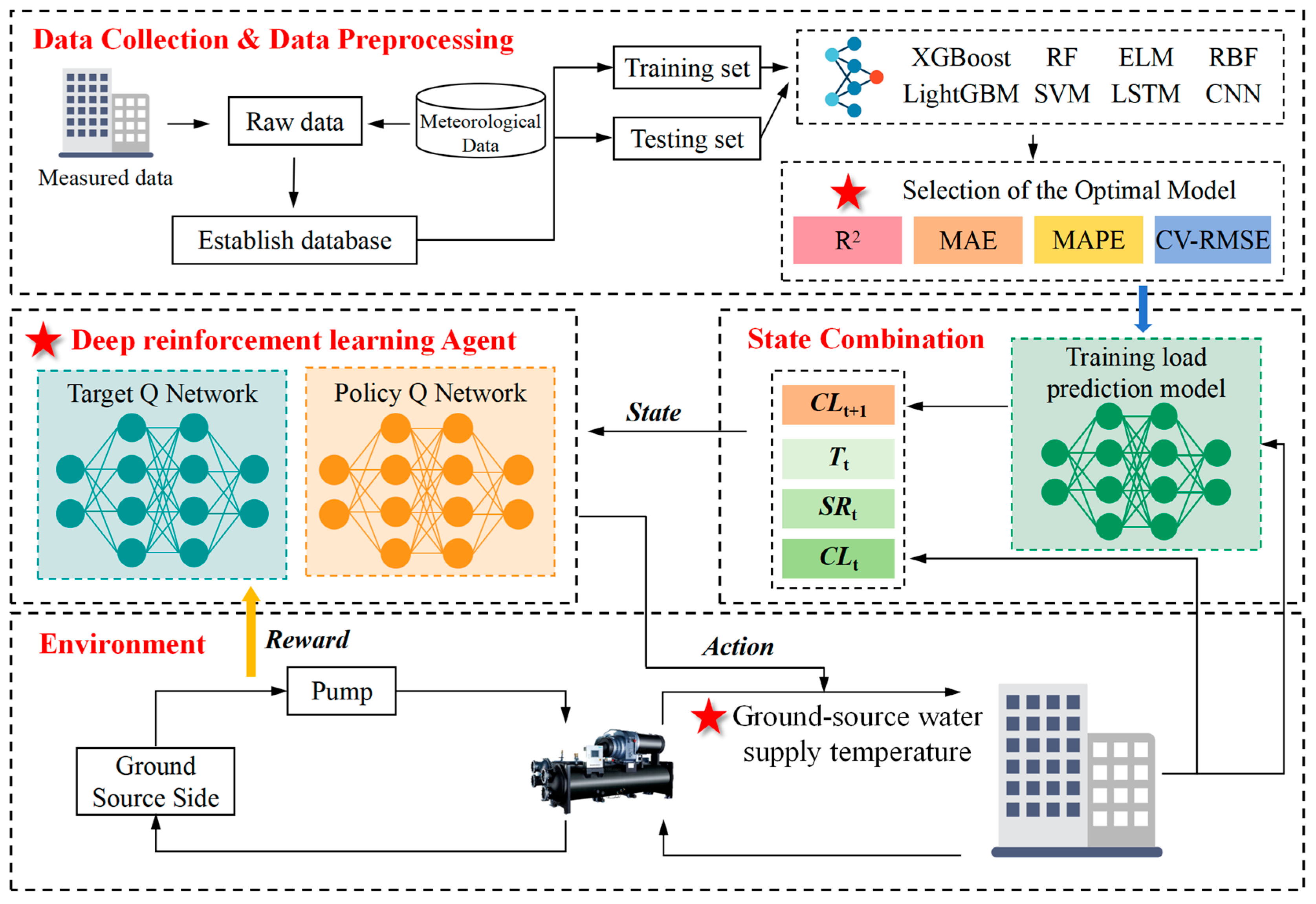
The technical roadmap of this study is illustrated in Figure 1. The proposed method combines deep reinforcement learning with load forecasting. Eight machine learning models are first trained to identify the most effective prediction model. The latter is then combined with reinforcement learning. During each control cycle, the selected model predicts the upcoming change in cooling load. This prediction is then combined with the current load and outdoor weather conditions to create a new quadruple state representation, which is then used as input for the deep Q-network. Based on this state, the agent optimizes the supply temperature at the geothermal end, and an immediate reward value is obtained by comparing the energy consumptions of the system before and after adjustment. The size of this reward value reflects the effectiveness of energy savings, which guides the agent toward learning more efficient energy-saving strategies.
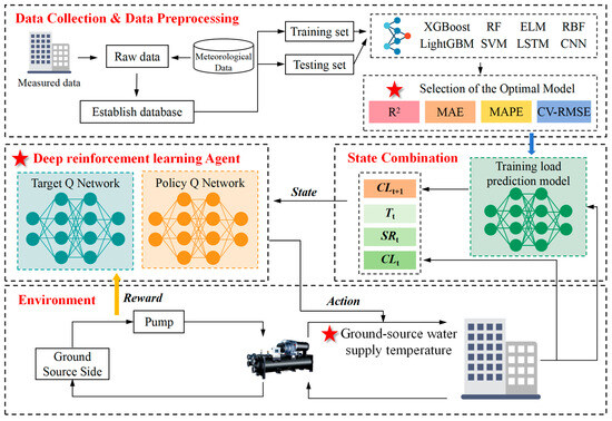
Figure 1.
Technical roadmap of the study.
2.1. Overview of Load Forecasting Models
This study evaluates eight machine learning models to identify the most suitable one for geothermal heat pump systems. These models comprise two boosting techniques (extreme gradient boosting and light gradient boosting machine), two deep learning methods (long short-term memory neural networks and convolutional neural networks), and four supervised learning algorithms (random forest, extreme learning machine, radial basis function neural network, and support vector machine). The learning capacities and characteristics of these algorithms are compared to identify the one having the highest accuracy. Due to the high complexity of the geothermal heat pump systems, the use of various models allows us to better understand the system behavior, and thus, helps the subsequent optimization procedures. By comparing the performances of these models, the most consistent one with the characteristics of geothermal heat pump systems is selected.
- (1)
- Extreme gradient boosting
Extreme gradient boosting (XGBoost) is a decision tree algorithm of high efficiency commonly used for classification and regression tasks [25]. It increases the generalization ability of the model by optimizing the objective function and incorporating regularization terms. It combines multiple simple decision trees to develop a robust prediction model, which allows for significantly reducing the risk of overfitting while also optimizing the computational efficiency. This makes it applicable to various scenarios of data analysis and mining [26]. The data prediction of XGBoost can be expressed as:
where represents the actual value, denotes the predicted value in the r-th iteration, represents the structure of the decision tree, represents the loss function, and is the regularization term given by:
where T represents the number of leaf nodes, w denotes their weights, λ and γ are coefficients having default values of 1 and 0, respectively.
- (2)
- Random forest
Random forest (RF) is an ensemble learning method usually used to solve classification, regression, and feature selection problems in machine learning [27]. It constructs a collection of decision trees by randomly selecting features and samples, while ensuring the independence of these trees. The final predictions are improved through a voting or averaging mechanism, which increases accuracy and stability. It has very high performance when dealing with large-scale and complex datasets. It has a wide application range due to its high versatility and robustness [28]. The RF prediction of the target variable, consisting of k decision trees, is expressed as:
- (3)
- Extreme learning machine
Extreme learning machine (ELM) is a learning algorithm for single-layer feedforward neural networks [29]. It randomly assigns input layer weights and hidden layer biases, and analytically calculates output layer weights. This design significantly increases the training speed while maintaining high generalization ability, which makes the ELM suitable for many machine learning problems [30]. ELM is mathematically expressed as:
where T, , and denote the activation functions.
- (4)
- Light gradient boosting machine
Light gradient boosting machine (LightGBM) is a gradient boosting framework based on decision trees. It increases the training speed and efficiency by employing a splitting strategy that prioritizes mutually exclusive leaf nodes and uses histogram-based acceleration techniques [31]. It is well-suited for handling high-dimensional data and large-scale datasets, achieving a balance between the accuracy and computational efficiency of the model [32]. LightGBM is given by:
- (5)
- Radial basis function network
Radial basis function network (RBF) is a three-layer feedforward neural network having a single hidden layer that employs radial basis functions as activation functions. Its architecture facilitates the nonlinear mapping from the input space to the hidden layer, as well as the linear mapping from the hidden layer to the output layer. It has high efficiency when tackling complex function approximation problems, and is less prone to the local minima problem faced by other networks [33]. The output of the network for an input x can be expressed as:
where yi(x) denotes the ith output of the RBF, wki is the weight connecting the kth hidden node to the ith output node, ||x − ck|| represents the Euclidean norm, and φ represents the Gaussian function.
- (6)
- Support vector machine
Support vector machine (SVM) is a machine learning algorithm based on the statistical learning theory, which makes it well-suited for small sample sizes [34]. By employing various kernel functions, SVM effectively handles linearly non-separable data [35]. Its least squares variant further increases the efficiency of solving optimization problems as well as the prediction accuracy of the model. Given a dataset (D = {(xi, yi) | i = 1, 2,…, l}), where xi represents the input, yi denotes the output, and l is the sample size, the regression aims at identifying the dependency of y on x from the sample data. Thus, an insensitive loss function (ε) is defined, and the linear insensitive loss function can then be expressed as:
where f represents the decision function which can be written for linearly separable datasets as:
where b denotes the bias term and w represents the weight vector.
- (7)
- Long short-term memory neural network
Long short-term memory (LSTM) networks are an advanced type of recurrent neural networks designed to overcome the vanishing gradient problem commonly faced by traditional recurrent neural networks when processing long sequences of data [36]. LSTMs incorporate mechanisms known as the forget gate, input gate, and output gate, which allow to learn and retain long-term dependencies. As a result, they have very high performance in many application domains, including time series forecasting and natural language processing, where the ability to capture long-range relationships is crucial.
- (8)
- Convolutional neural network
Convolutional neural networks (CNNs) are a type of deep feedforward neural networks. Their architecture comprises convolutional and pooling layers, providing significant advantages in many fields, such as image recognition, video analysis, and speech recognition [37]. They employ hierarchical feature extraction and abstraction to effectively process high-dimensional data inputs while decently dealing with the complexity of the underlying model. In the convolutional layer, the convolution operation processes the input data as follows:
where Wi denotes the weight tensor serving as the convolution kernel, * represents the convolution operation, ai−1 is the output from the (i − 1)-th layer, bi is the bias for the ith layer, zi represents the linear output before activation at the ith layer, f is the activation function, and ai is the activated output of the ith layer.
2.2. Reinforcement Learning
Reinforcement learning is a process where an agent interacts with an uncertain environment to maximize cumulative rewards. This is typically represented by a Markov Decision Process (MDP) characterized by states (S), actions (A), rewards (R), transition probabilities (P), and discount factor (γ) [38]. In the context of deep Q-networks, neural networks are used to approximate the state-action value function Qπ(s, a). More precisely, the neural network takes the state and action as inputs and outputs the corresponding Q-value [15]. The iterative updating process is given by:
where π represents the policy, α denotes the learning rate, and γ is the discount factor.
Several key techniques are employed to make the leaning process more stable and efficient:
- (1)
- The policy Q-network and target Q′-network, having the same architecture and initial parameters, are used to stabilize the update of the Q-function.
- (2)
- In order to balance the exploration and exploitation, a ε-greedy strategy is adopted for action selection. The agent randomly selects actions with a probability of ε, which gradually decreases to εmin over time at a rate of Δε.
- (3)
- After executing an action, the agent stores the ((s, a, r, s′)) experience tuple in a replay memory.
- (4)
- When a state ends, a mini-batch of experiences is randomly sampled from the replay memory to update the parameters of the network, while prioritized experience replay is used to increase the learning efficiency.
3. Case Study
3.1. Load Prediction Using Different Machine Learning Algorithms
3.1.1. Data Collection
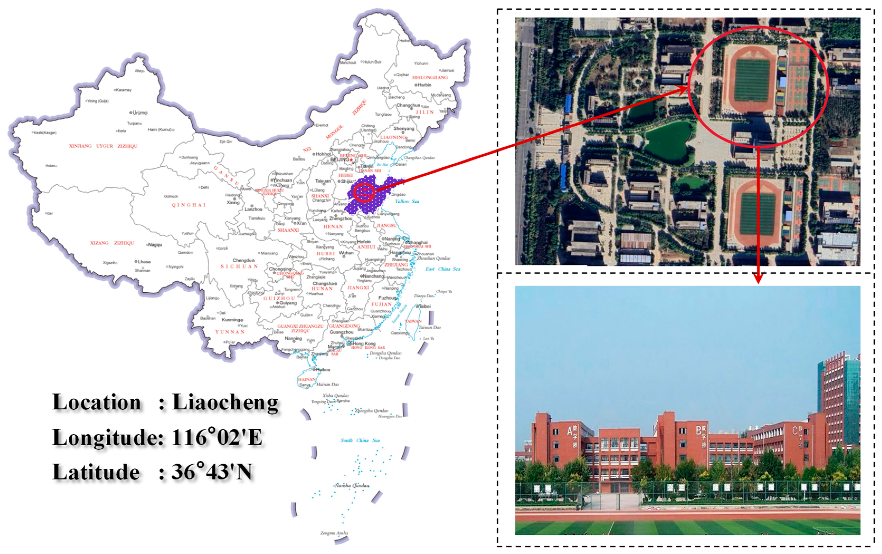
This paper considers the underground geothermal heat pump energy station of a comprehensive building at a school in Liaocheng (China) as the study object. The facility has an area of 23,000 m2 and a building height of 48.75 m. The main building contains a basement used for equipment storage, having an area of 700 m2. It has 12 above-ground floors, having a total area of 14,000 m2. A three-story annex building, having an area of 9000 m2, also exists, as shown in Figure 2. The actual air conditioning coverage area is 16,000 m2. Considering the local climate conditions, the air conditioning system is designed to have cooling and heating loads of 1900 kW and 1800 kW, respectively. The geothermal heat pump unit is the source for heating and cooling. Table 1 shows the main equipment and performance parameters of the energy station.

Figure 2.
Geographical location and exterior view of the building.

Table 1.
Main equipment and performance parameters of the energy station.
The energy station is equipped with an intelligent remote monitoring and management platform that continuously tracks parameters, such as water temperature, power consumption, and water flow rate. These data are transmitted to a smart control center for the intelligent regulation of the equipment. The system is able to perform data visualization, which allows the users to monitor real-time status and metrics, which are finally uploaded to the cloud through a remote module. Monitoring data, recorded every 30 min, allows for querying, displaying, storing, and analyzing information, which facilitates the energy consumption analysis and the increase in energy efficiency. The data upload function promotes the commitment of the energy station to green and sustainable development, while effectively managing carbon emissions. In summary, the intelligent remote monitoring system of the geothermal heat pump energy station is highly functional. It allows for the comprehensive surveillance and intelligent management of the air conditioning system, which optimizes energy efficiency, reduces energy consumption, and fosters sustainable development.
3.1.2. Data Preprocessing
Due to the fact that the dataset is collected by sensors, it contains outliers and missing values that necessitate appropriate data preprocessing. For missing data, interpolation techniques are used to maintain data integrity. During the data cleaning phase, the 3σ principle is used to identify and interpolate outliers, while also ignoring long-term repetitive or missing data to enhance the quality of the data. Furthermore, during the process of model training, regularization techniques are applied to reduce the sensitivity of the model to noise, which allows for increasing its generalization ability.
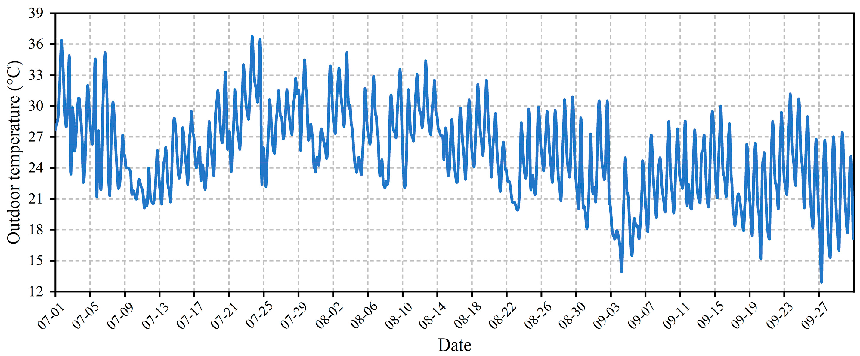
A case study was then conducted. Data were collected from the geothermal heat pump system at a comprehensive building in Liaocheng, China, covering a period from 1 July to 30 September 2023, totaling 92 days. The cooling load data of the building is illustrated in Figure 3. The variation in the outdoor solar radiation is presented in Figure 4. The outdoor temperature is illustrated in Figure 5.
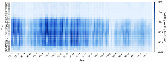
Figure 3.
Data of building cooling load.
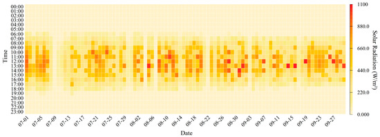
Figure 4.
Data on outdoor solar radiation.

Figure 5.
Data of outdoor wet bulb temperature.
3.1.3. Feature Selection
The cooling load of a building is affected by internal and external factors. Due to the lack of internal information in the studied building, this study focuses on analyzing the impact of the external disturbances on the cooling load. The selected input variables for the predictive model include the current system cooling load, outdoor wet bulb temperature, outdoor relative humidity, outdoor solar radiation, wind direction, and wind speed. The relevant features are presented in Table 2. To validate the effectiveness and robustness of the proposed prediction model, the data are divided into a training set (80%) and a testing set (20%).
Table 2.
Representation of feature parameters.
3.1.4. Hyperparameter Settings for Predictive Models
The optimal input parameters for each model, adopted in Matlab, are summarized in Table 3.
Table 3.
Key hyperparameter settings for predictive models.
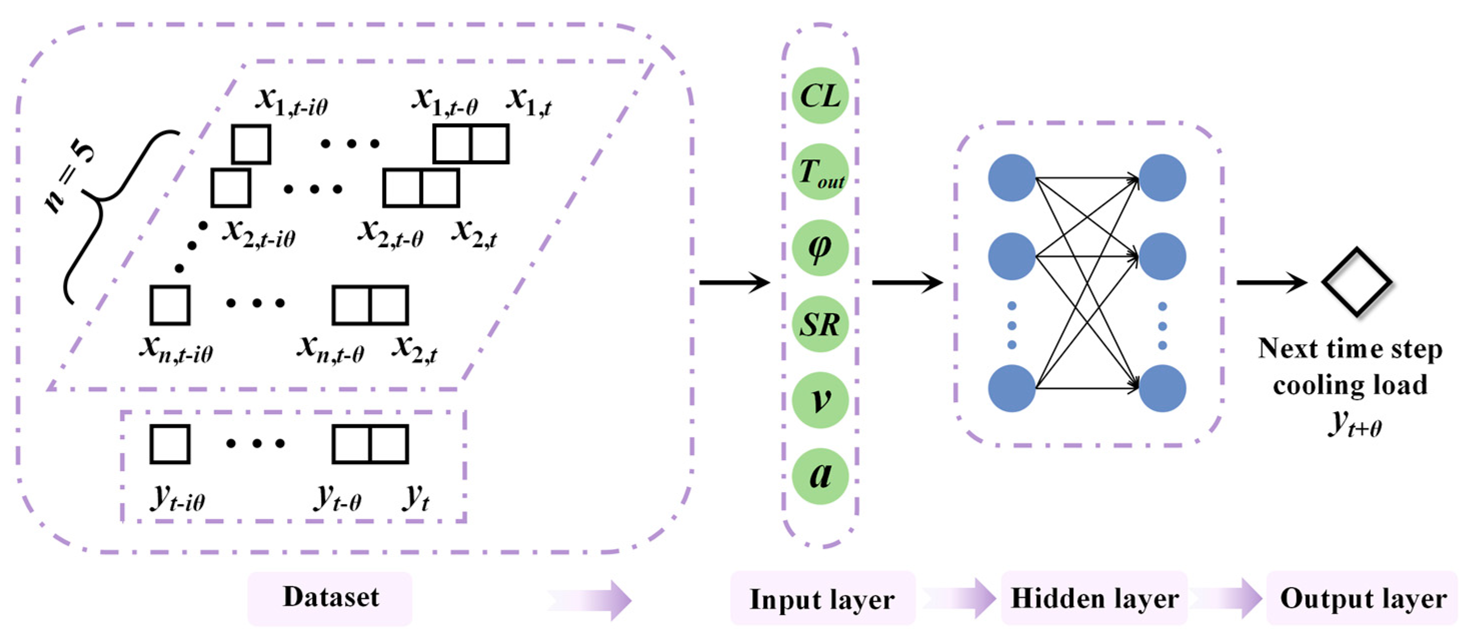
Figure 6 shows the used neural network predictive structure, where six selected features are incorporated. The current value of each feature is denoted by xm,t, where m and t represent the feature index and current time instance, respectively. Note that xm,t-iθ denotes the value of the feature at a previous time interval, and θ represents a duration of 30 min.
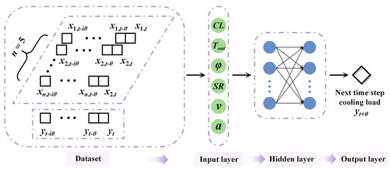
Figure 6.
Neural network structure for building cooling load prediction.
For the purpose of machine learning forecasting, the data must be converted into a time series format, represented as Μt:
where CLt represents the cooling load at time t (kW), Tout denotes the outdoor temperature (°C), φ represents the relative humidity, SR denotes the solar radiation (W/m2), v is the outdoor wind speed (m/s), and α is the wind direction (degrees).
3.1.5. Evaluation Metrics
Four metrics are used to evaluate the accuracy of the prediction models: the Coefficient of Determination (R2), Mean Absolute Error (MAE), Mean Absolute Percentage Error (MAPE), and Coefficient of Variation in the Root Mean Squared Error (CV-RMSE) [39]:
where n represents the number of samples, xi denotes the ith simulated value (kW), yi denotes the ith actual measurement (kW), represents the mean of the simulated values (kW), and represents the mean of the actual measurements (kW).
These metrics allow for systematically comparing the learning capacities and characteristics of the algorithms. This enables the identification of those with superior prediction accuracy. R2 quantifies how accurately the prediction model fits the observed data. Its values are in the range of 0–1. A value close to 1 indicates that the prediction is very consistent with the actual data, while a value of 0 indicates a very low prediction accuracy, which is almost equivalent to considering the average of the output variable as the predicted value. MAPE reflects the ratio of MAE to the average value of the output variable, while CV-RMSE denotes the relative magnitude of the root mean square error compared with the average value of the output variable. They both indicate an optimal value when reaching 0. R2, MAPE, and CV-RMSE are all dimensionless. They effectively incorporate the complexity of the output variable and the inherent difficulty of the regression task, which allows for overcoming the limitations of the dimensioned evaluation metrics.
3.2. Deep Reinforcement Learning Optimization Control
3.2.1. Model Establishment Process
In this case study, the states, actions, and rewards are defined as follows:
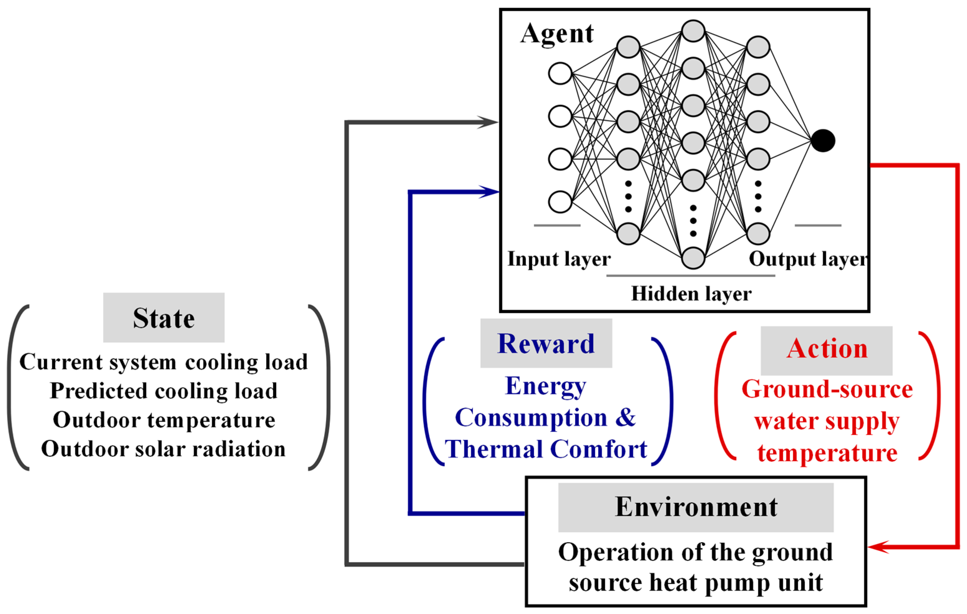
(1) State: It is defined as a combination of four operational variables: the current system cooling load (CLt), predicted cooling load (CLt+1), outdoor wet bulb temperature (Tout), and outdoor solar radiation (SR).
(2) Action: In the reinforcement learning framework, it is the setting of the ground-source supply water temperature, with a control interval of 1 °C. The temperature setting range is determined by the equipment nameplate, typically equal to 5–13 °C.
(3) Reward: The setting of the ground-source supply water temperature significantly affects the energy consumption and cooling capacity. It is crucial to enhance energy efficiency while ensuring indoor comfort. Thus, based on an extensive review of relevant literature, a comprehensive reward structure that balances energy consumption with comfort is adopted, as represented in Equation (16) [7]:
where α and β, respectively, represent the weights for energy consumption and comfort with a constraint of α + β = 1, Popt denotes the optimized energy consumption of the ground-source heat pump unit, and Pref represents the rated energy consumption. Note that the difference between the ground-source supply water temperature (Tground) and the upper limit of the ground-source supply water temperature (Tground,ref) reflects whether the provided cooling capacity is adequate. The μ1 and μ2 coefficients are determined through regression analysis. A detailed description of the Markov decision process is illustrated in Figure 7.
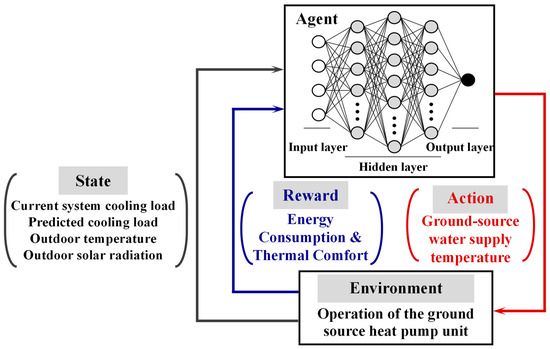
Figure 7.
Description of the Markov decision process.
3.2.2. Hyperparameter Configuration for the Deep Q-Network
The hyperparameter settings of the used deep Q-network are presented in Table 4. The model was trained for approximately 2 h, where each training episode consisted of 300 cycles of 1000 iterations each. The determination of cycles and iterations was based on the need to ensure that the model can learn the optimal policy across a sufficient range of state variations. More precisely, the 300 training cycles aimed at performing policy convergence for each state group, while the 1000 sets of continuous state inputs simulated dynamic changes in a real-world environment. This allowed us to enhance the adaptability of the model in complex scenarios. During the training process, regularization techniques were employed to mitigate the risk of overfitting. These techniques were applied to reduce overfitting and increase the generalization ability of the model.
Table 4.
Hyperparameter settings for the deep Q-network.
3.2.3. Comparative Strategy Configuration
In the simulation experiments, the load forecasting-based deep reinforcement learning control method was compared with three other methods: a deep reinforcement learning control method without predictive information, an empirical formula method, and a constant water temperature control method. The detailed configurations of the four control strategies are described as follows:
(1) Strategy 1: It uses a load forecasting-based deep reinforcement learning method. It employs a prediction model to forecast the future trends of cold load based on historical data, incorporating a reinforcement learning framework to optimize the control strategy. During the decision-making process, the agent considers the current cold load state and the anticipated future cold load (S = [CLt, CLt+1, Tout, SR]).
(2) Strategy 2: It implements a deep reinforcement learning control method that does not use predictive information. It selects control actions based only on the current state (S = [CLt, Tout, SR]), while all the other procedures mirror those of Strategy One, which relies on predictions.
(3) Strategy 3: It develops a simulation model using empirical formulas and precise parameters. At each simulation step, the model receives state inputs as defined in Strategy One (S = [CLt, CLt+1, Tout, SR]).
(4) Strategy 4: It employs a constant water temperature control method, setting the chilled water supply temperature at a constant value of 7 °C based on recommended parameters from equipment manufacturers, without taking real-time variations in cold load into consideration.
4. Results
4.1. Performance Analysis of the Prediction Models
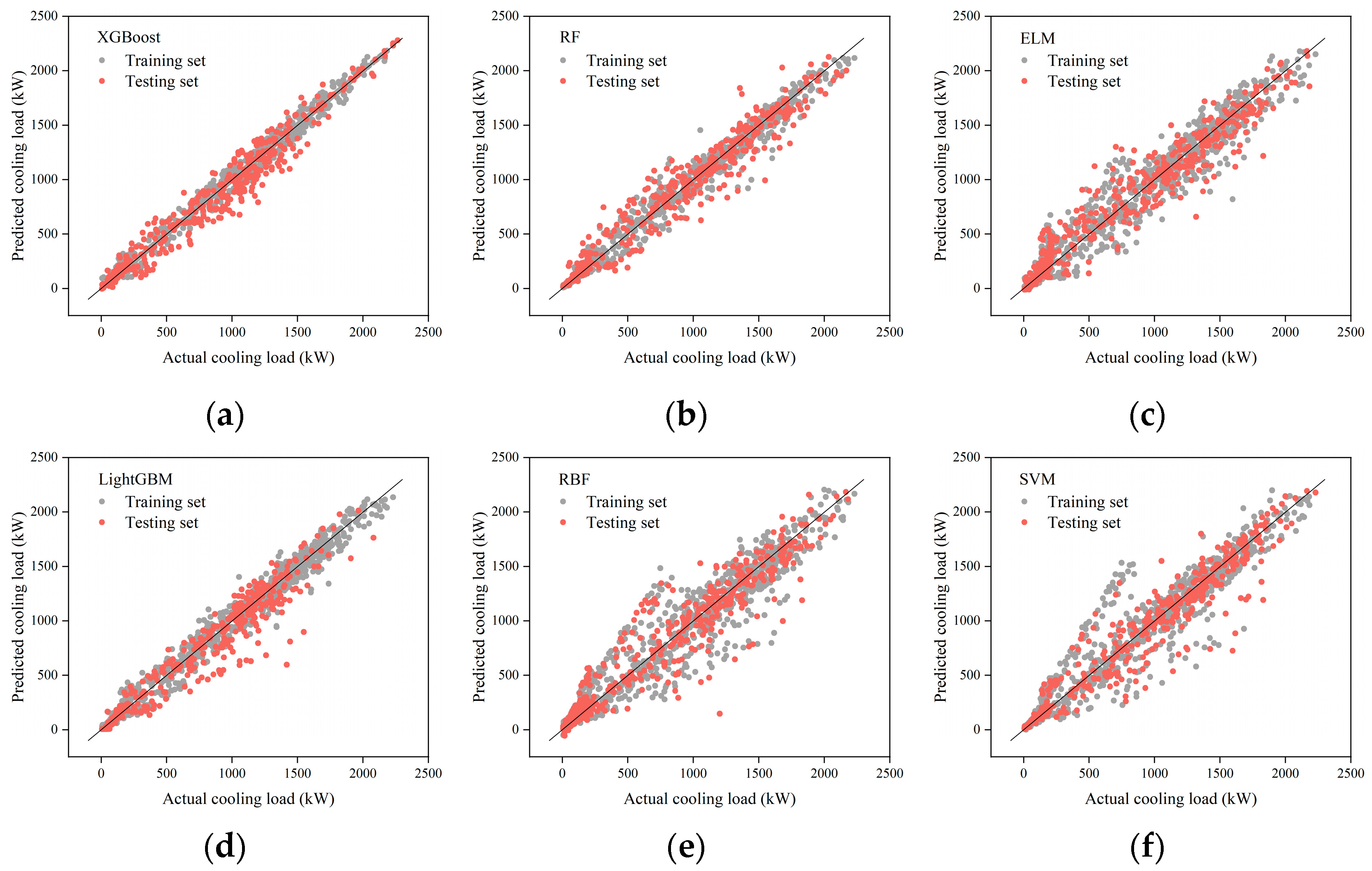
The R2, MAE, MAPE, and CV-RMSE were used to comprehensively evaluate the prediction abilities of the eight models. The obtained results are presented in Table 5. Figure 8 illustrates a comparison between the predicted values and the actual values for all the models. It can be seen from Table 5 that the MAPE and CV-RMSE values for the ELM, RBF, SVM, LSTM, and CNN models are all greater than 15%, which indicates significant errors in their predictions. Furthermore, it can be observed from Figure 8 that significant differences exist between the predicted and actual values for these five models, which do not closely adhere to the reference line \( y = x\) . Consequently, they have low prediction performance, and thus, they are not recommended for cold load forecasting in this case study.
Table 5.
Prediction results obtained by different models.
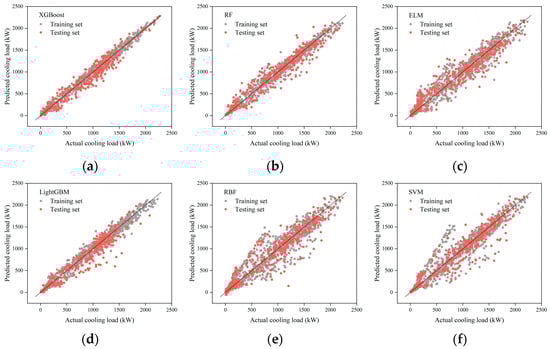

Figure 8.
Comparison between the prediction performances of different models: (a) XGBoost, (b) RF, (c) ELM, (d) LightGBM, (e) RBF, (f) SVM, (g) LSTM, (h) CNN and (i) Comparison of CV-RMSE for different models.
On the contrary, the XGBoost, RF, and LightGBM models have very high performance, achieving the highest metrics, reaching an R2 value greater than 0.97. Both XGBoost and LightGBM use boosting techniques, underscoring the significant potential of such methods for the accurate prediction of building cold loads. These three models have very high prediction abilities, and thus, they are well-suited for cold load forecasting.
The very high performance of the XGBoost model is mainly due to its efficient ensemble method of decision trees. By constructing and combining multiple decision trees, XGBoost employs gradient boosting techniques to optimize the performed predictions and incorporates regularization terms to prevent overfitting, which ensures the high generalization ability of the model [40]. Its structure allows XGBoost to accurately handle data with deep feature associations, especially in scenarios that require high prediction accuracy and model interpretability [41].
The core strength of the RF model lies in its ensemble learning strategy and very high resistance to overfitting [42]. By randomly selecting features and samples to train multiple decision trees, RF captures various patterns within the data and increases the prediction stability and accuracy through a voting mechanism among the trees. This model is very effective when dealing with highly complex and noisy datasets due to its high robustness and tolerance for outliers.
LightGBM is known for its high training speed and ability to handle high-dimensional data [27]. It employs a histogram-based binning method, combined with a leaf-wise exclusive strategy and gradient-based one-side sampling technique. This significantly reduces the computational load and accelerates the convergence, which allows it to rapidly and accurately capture key features within the data during prediction tasks. This increases the computational efficiency while maintaining high prediction performance.
Furthermore, it can be observed that the RBF and SVM models undergo instances of overestimation in their load curve predictions. This phenomenon occurs because these prediction models cannot accurately capture the fluctuating trends of cold load during periods of very high variability.
Among all the models, XGBoost achieves the highest R2 and the lowest metrics. Therefore, it is considered the most effective algorithm for prediction. Compared with the models of lower performance, its MAPE and CV-RMSE are, respectively, reduced by 80.87% and 53.36%, which demonstrates its higher prediction accuracy. Therefore, this paper proposes to incorporate the XGBoost prediction model into the next phase of the proposed reinforcement learning optimization control.
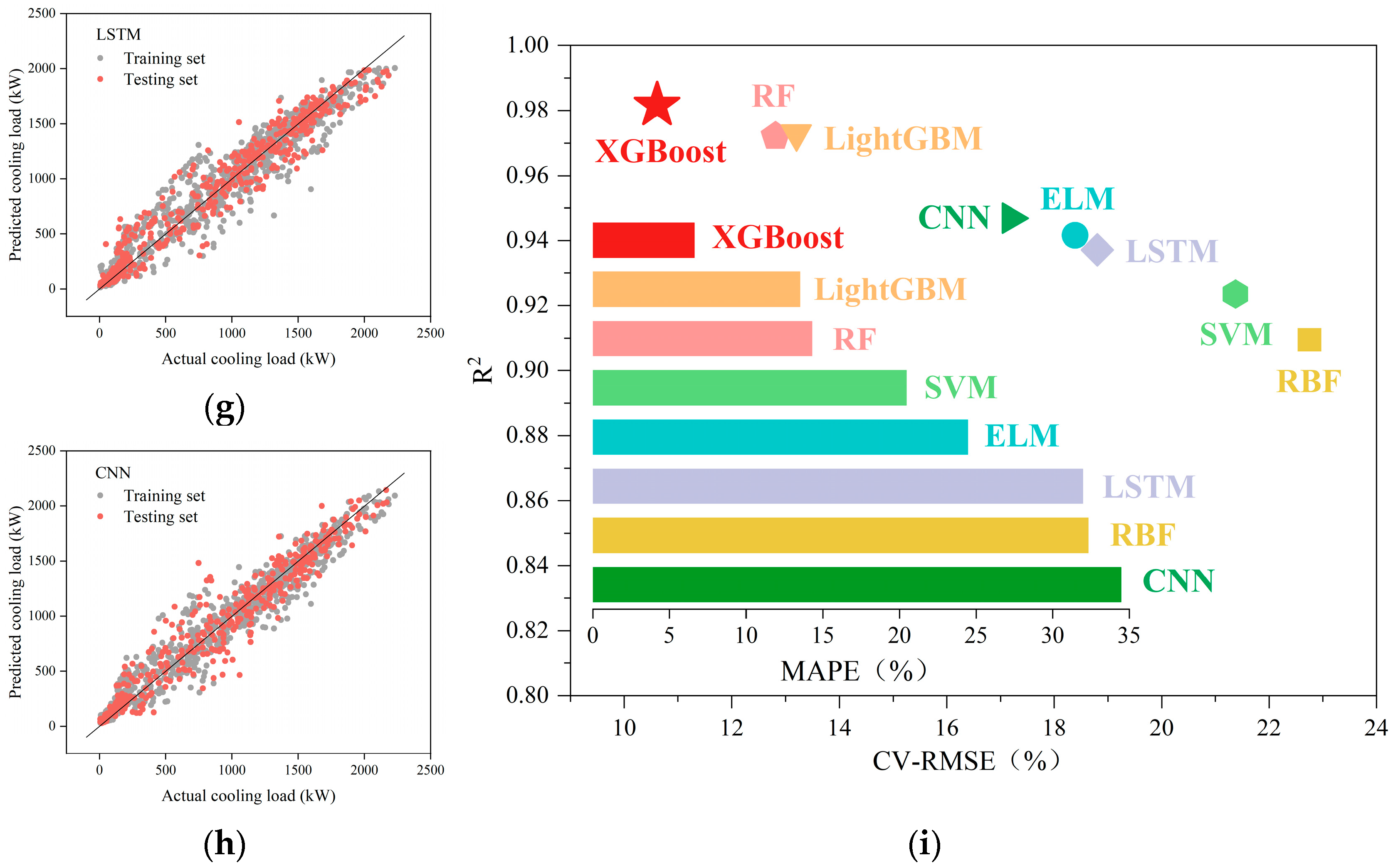
Figure 9 illustrates the normal distribution of the prediction errors obtained by the different models, with a distinction made between the training and testing sets. Note that the horizontal line in the box plot represents the median of the errors, while the star denotes the mean error. It can be seen that, except for the XGBoost model, the errors for the other models are mainly less than zero, which indicates a tendency to overestimate the cold load. During the testing phase, the models have a greater number of outliers and a wider range of errors, which indicates high uncertainty in predictions with new datasets. However, the normal distribution curves for all the models maintain a significant level of consistency between the training and testing sets. This demonstrates that, although the prediction accuracy varies, the methods of data processing across the models are almost similar.

Figure 9.
Normal distribution of errors for all the models: (a) training set and (b) testing set.
4.2. Performance Analysis of Reinforcement Learning
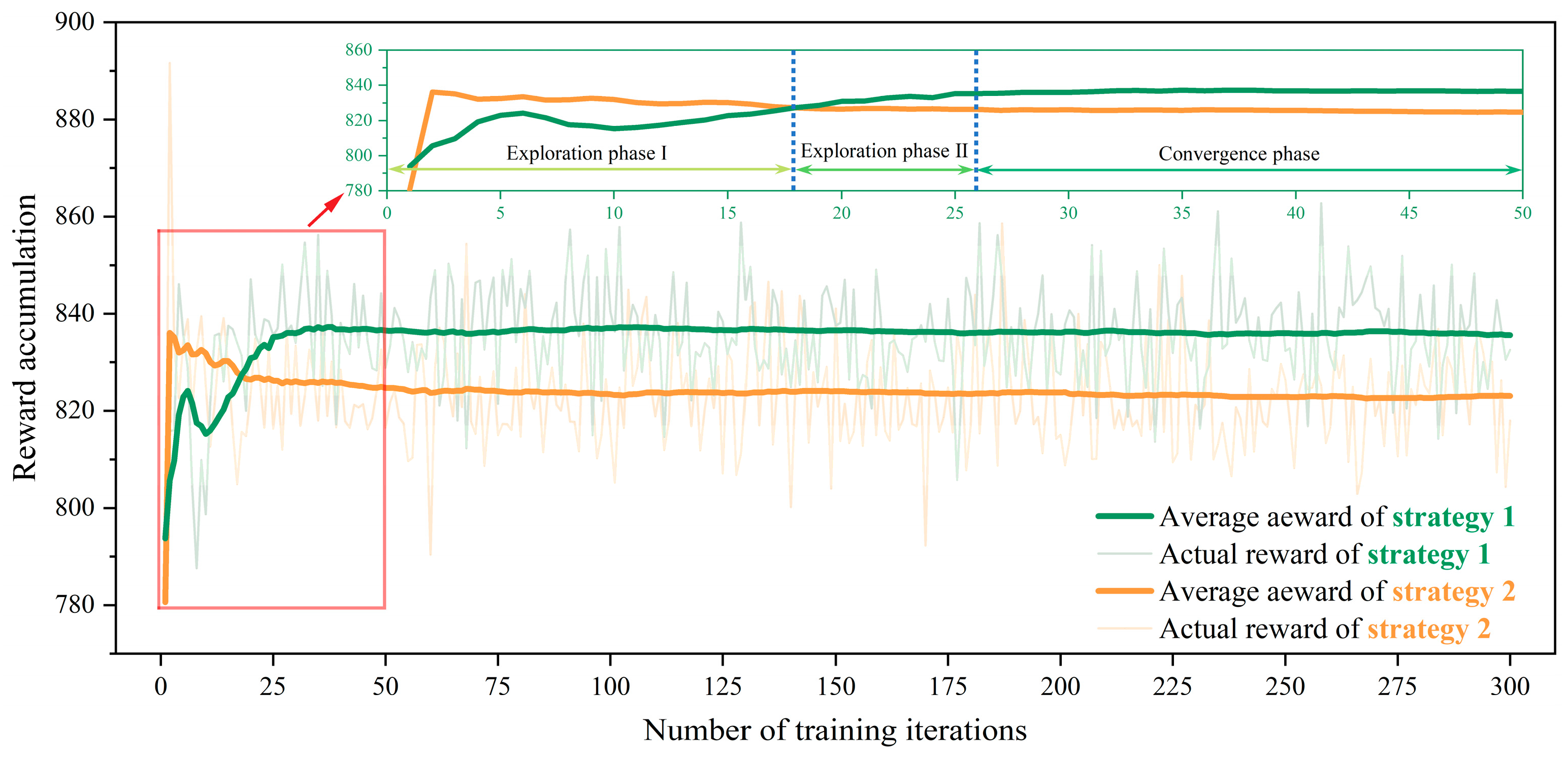
Figure 10 presents the trend of cumulative rewards for Policy One and Policy Two during the training process. It can be seen that in the initial 26 training episodes, the two policies have an increasing trend in cumulative rewards. This indicates that the agent continuously learns and refines its control strategy through interactions with the environment. Policy One incorporates current and future states in its action selection process, which results in a more experimental training phase during the early rounds, as illustrated in Phase I of exploration in Figure 10. Consequently, during this period, the cumulative rewards for Policy One are slightly lower than those for Policy Two. After the 26th training episode, the rewards for the two policies started to stabilize, with Policy One achieving higher cumulative rewards, which demonstrates its very high control performance. It is important to mention that the rewards for Policy One also exhibit some fluctuations, which may be attributed to the impact of the prediction accuracy. It can be observed from Figure 10 that the agent enters a state of convergence after the 50th training episode. This moves the focus to the analysis of the performance during the first 50 training episodes.
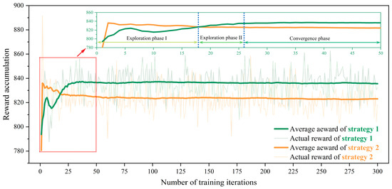
Figure 10.
Changes in cumulative rewards for Strategies 1 and 2 during each training episode.
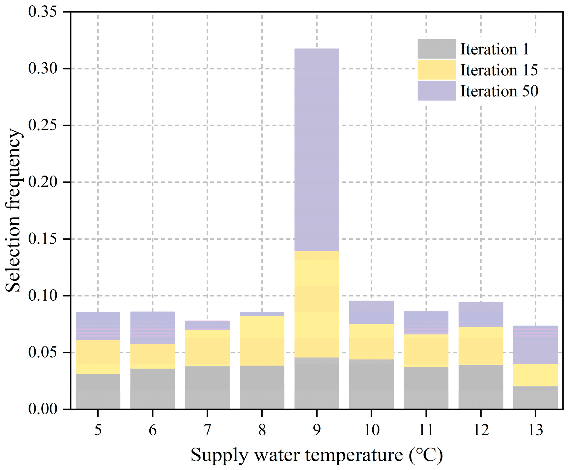
4.3. Analysis of the Source-Side Water Supply Temperature Setpoint
Figure 11 illustrates the selection frequency of actions related to the source-side water supply temperature for different training episodes using the proposed method. During the initial stages of training, the method employs a large number of exploratory actions, which results in a uniform distribution of temperature choices. When the Q-values are updated, and the ε-greedy mechanisms are decayed, the agent gradually starts to favor actions with higher Q-values, ultimately converging to the optimal solution. The optimal action for the source-side water supply temperature is approximately 9 °C, as shown in Figure 10. This can be considered a balance that conserves energy and meets the requirements of the end user.
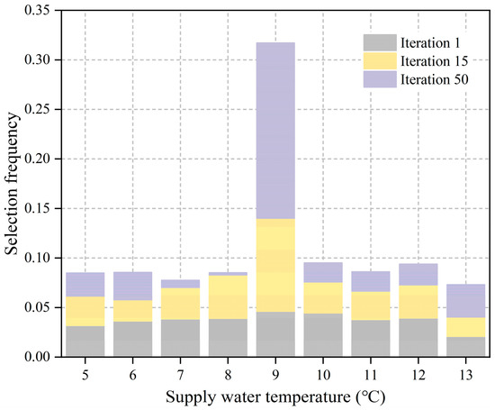
Figure 11.
Distribution of the selection frequency for the source-side water supply temperature during the iterative process.
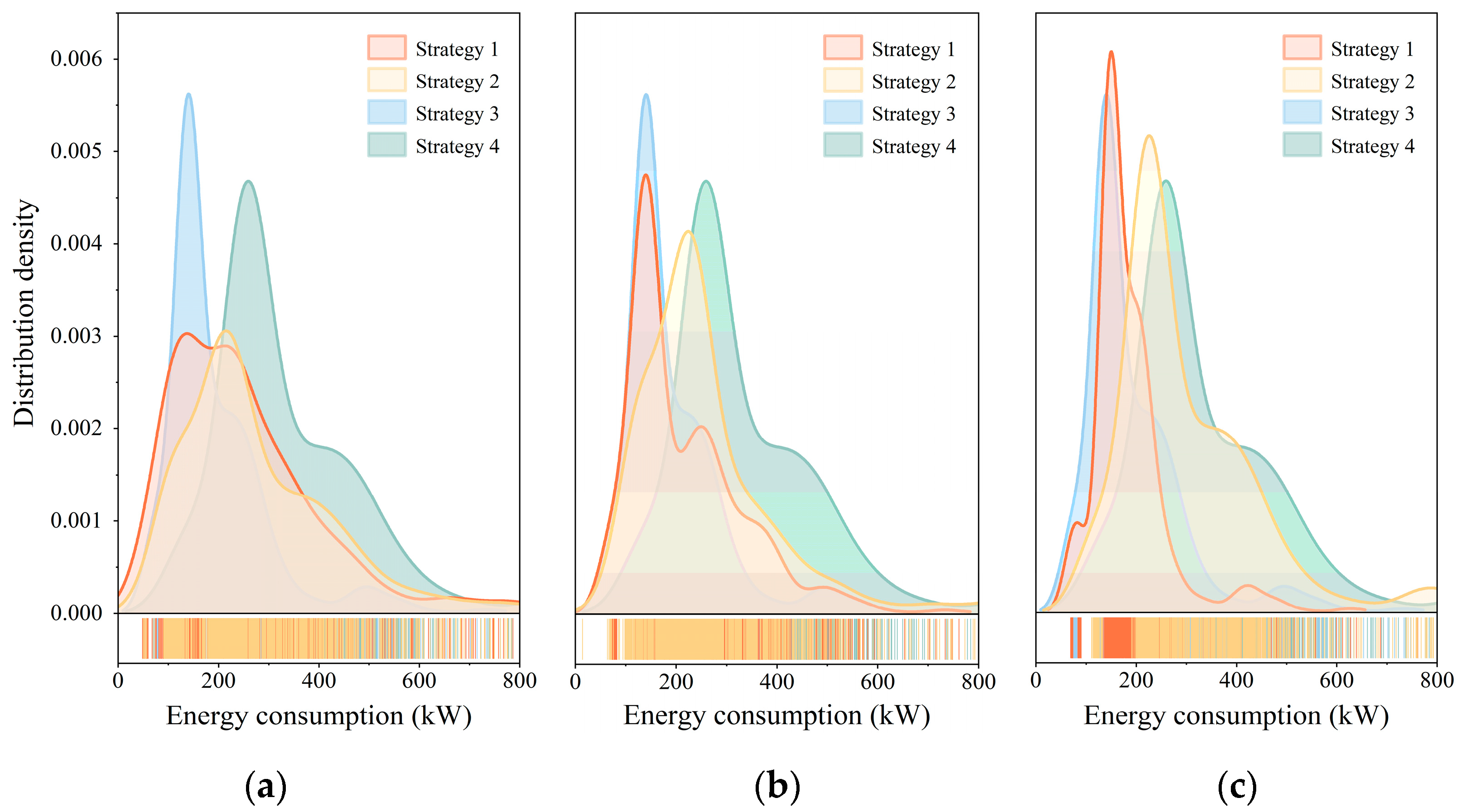
4.4. Energy Consumption Analysis of Ground Source Heat Pump Units
Figure 12 illustrates the trend of energy consumption of ground source heat pump units over training iterations, when different control strategies are employed. In Strategy Four, a rule-based control method is implemented, setting the supply water temperature for the ground source side low. As a result, the energy consumption of the ground source heat pump unit consistently remains close to its rated power. On the contrary, Strategy Three uses an empirical formula model, which incorporates a certain level of understanding of the actual system, which allows for adjusting the control strategy in response to environmental changes. Consequently, the energy consumption of the ground source heat pump unit under this strategy is maintained within the range of 125–200 kW over an extended period.
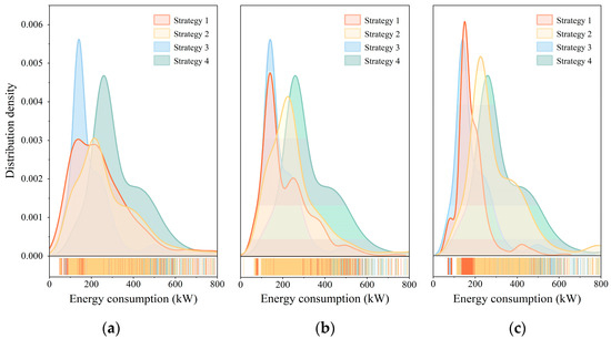
Figure 12.
Energy consumption distribution for different control methods: (a) 1st iteration, (b) 20th iteration, and (c) 50th iteration.
On the contrary, Strategies One and Two are engaged in extensive exploration during the initial training phase, which leads to a more dispersed distribution of energy consumption. However, as the training progresses, the energy consumption of the two control methods gradually concentrates in the low-energy consumption area. By the 20th iteration, the energy consumption distribution starts to converge, and by the 50th iteration, the distribution of energy consumption for Strategy One is very consistent with Strategy Three. The analysis of the energy consumption distribution shows that, due to the incorporation of the predictive information in Strategy One, most of the time, its energy consumption is lower than that of Strategy Two, with significantly fewer instances of high power consumption. This demonstrates that the incorporation of predictive information allows for significantly increasing the energy performance of control strategies.
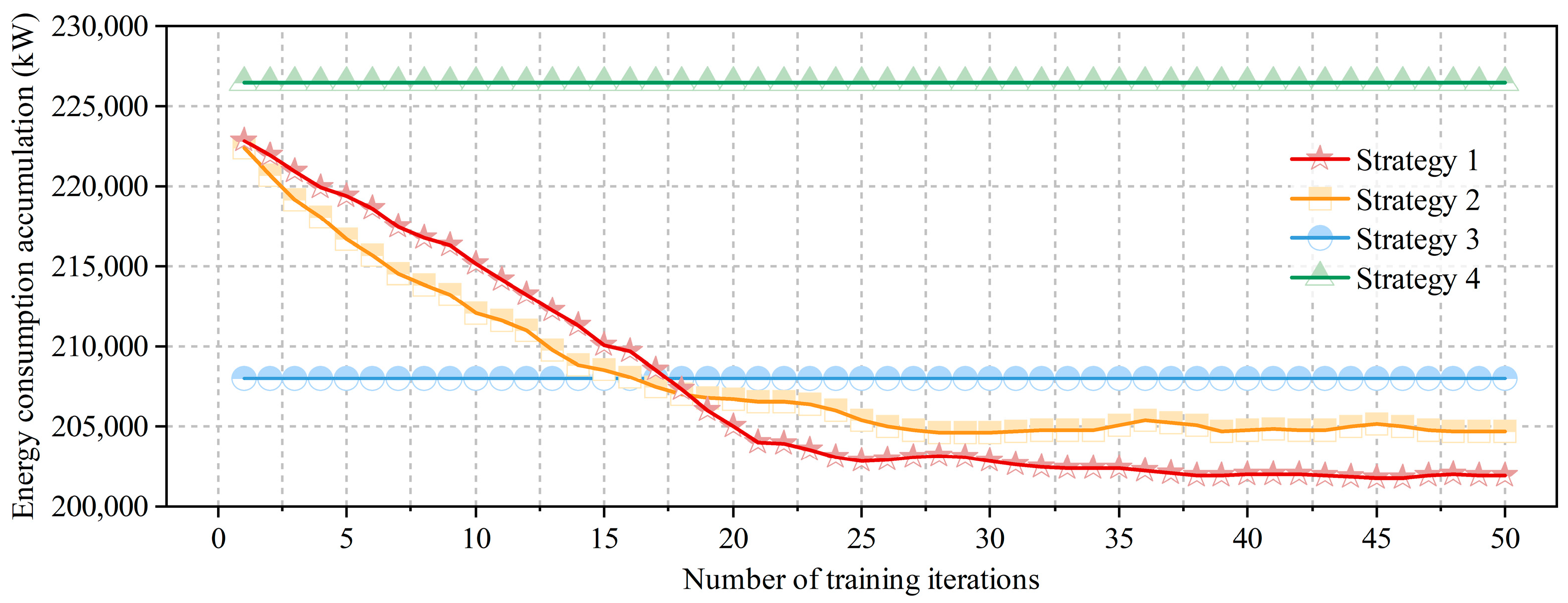
Figure 13 illustrates the cumulative energy consumption of four control methods during the first 50 training iterations. It can be seen that Strategy One is more energy-efficient than Strategy Four, while it is slightly less efficient than Strategy Three. Furthermore, compared with Strategy Two, Strategy One has lower energy consumption in the later stages of training. This demonstrates that the incorporation of predictive information can significantly increase the energy efficiency of the system without reducing the control interval.
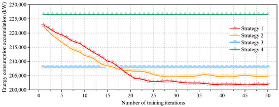
Figure 13.
Cumulative energy consumption of four control methods during the first 50 training iterations.
Using Strategy 4 as a benchmark, the energy-saving effectiveness of the other three control methods are compared during the first 50 training iterations. Strategies 1 and 2 employ learning and exploration mechanisms, which results in progressively higher energy savings as training advances, until they reach a state of convergence. In general, Strategy 1 achieves a higher energy-saving rate (0.38%) than Strategy 2. This difference is due to the fact that the system energy consumption for the two methods overlaps most of the time, with significant differences emerging mainly during periods of drastic changes in cooling load. When the cooling load slowly varies, the supply water temperature from the ground source remains constant. However, in the case of a sudden increase in cooling load, the predictive reinforcement learning control method preemptively sets a lower supply water temperature to maintain indoor comfort. This results in slightly higher energy consumption compared with the non-predictive reinforcement learning control method. Strategy 3 achieves an energy-saving effect of 8.17%, which is attributed to the incorporation of precise parameters of the equipment within the empirical model. This model conducts comprehensive value calculations for all the potential actions prior to each control adjustment. As a result, Strategy 3 demonstrates significant energy-saving advantages during the early stages of the reinforcement learning training process. However, as the reinforcement learning process gradually converges, Strategies One and Two start to have high performance, outperforming Strategy 3.
5. Discussion
The optimization control of HVAC systems presents a complex nonlinear challenge. This study proposes a control method that incorporates deep reinforcement learning and load prediction. This allows for achieving significant energy savings through the optimization of ground-source supply water temperature. However, several issues should be further studied, and improvements should be made within practical engineering applications.
Due to the continuous advancement of artificial intelligence technologies, hybrid algorithms, GA-BP and MEA-BP may exhibit higher performance compared with singular algorithms. This is due to the fact that they leverage the advantages of multiple approaches [43,44,45]. In future work, the operational parameters of actual ground-source heat pump systems should be used to develop singular and hybrid models for the main energy-consuming components of the system, including unit energy consumption and user pump energy consumption. The LSTM, SVM, RF, ELM, CNN, BP, GA-BP, and MEA-BP models will be taken into consideration. A comprehensive comparison between the metrics of these eight prediction models will be conducted.
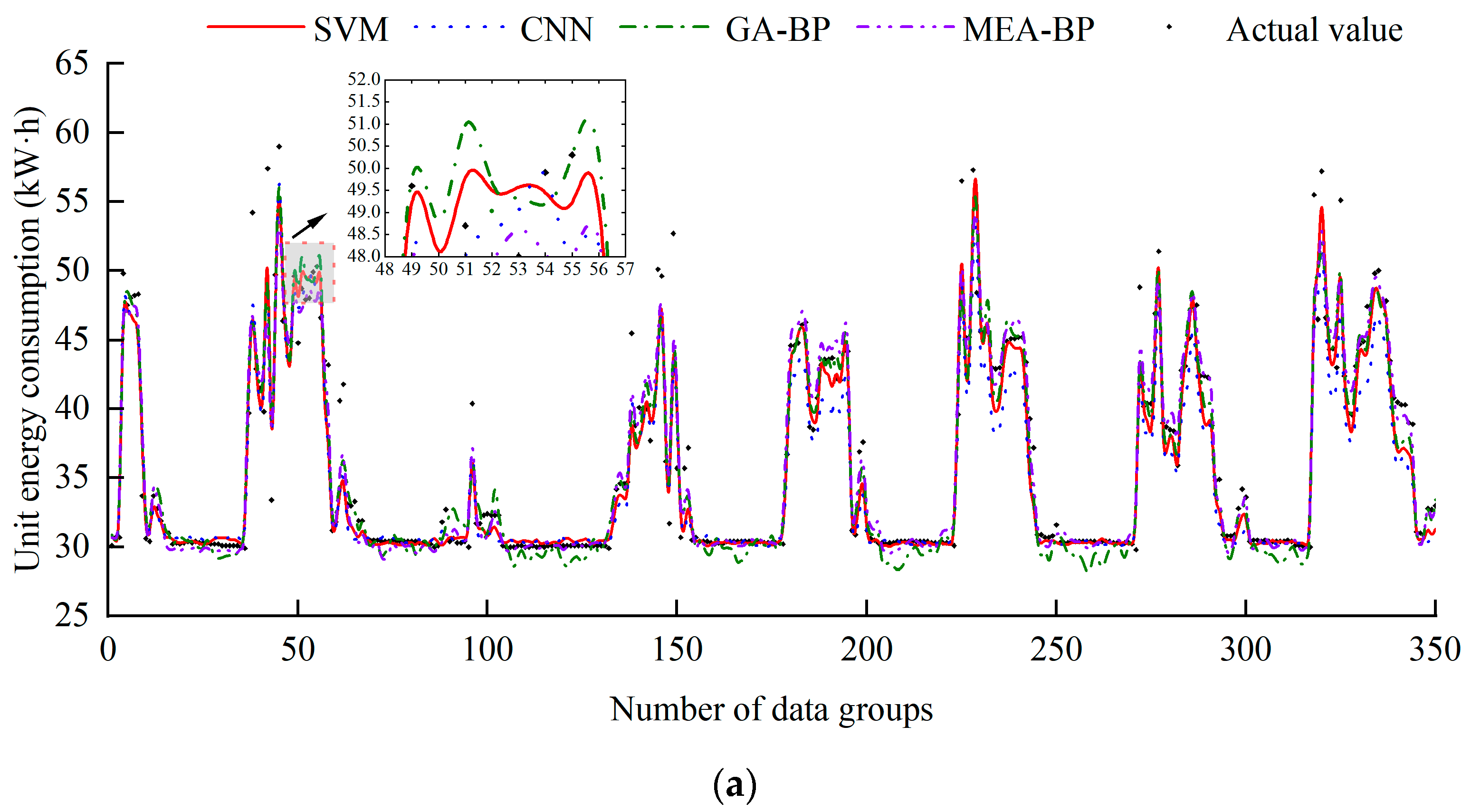
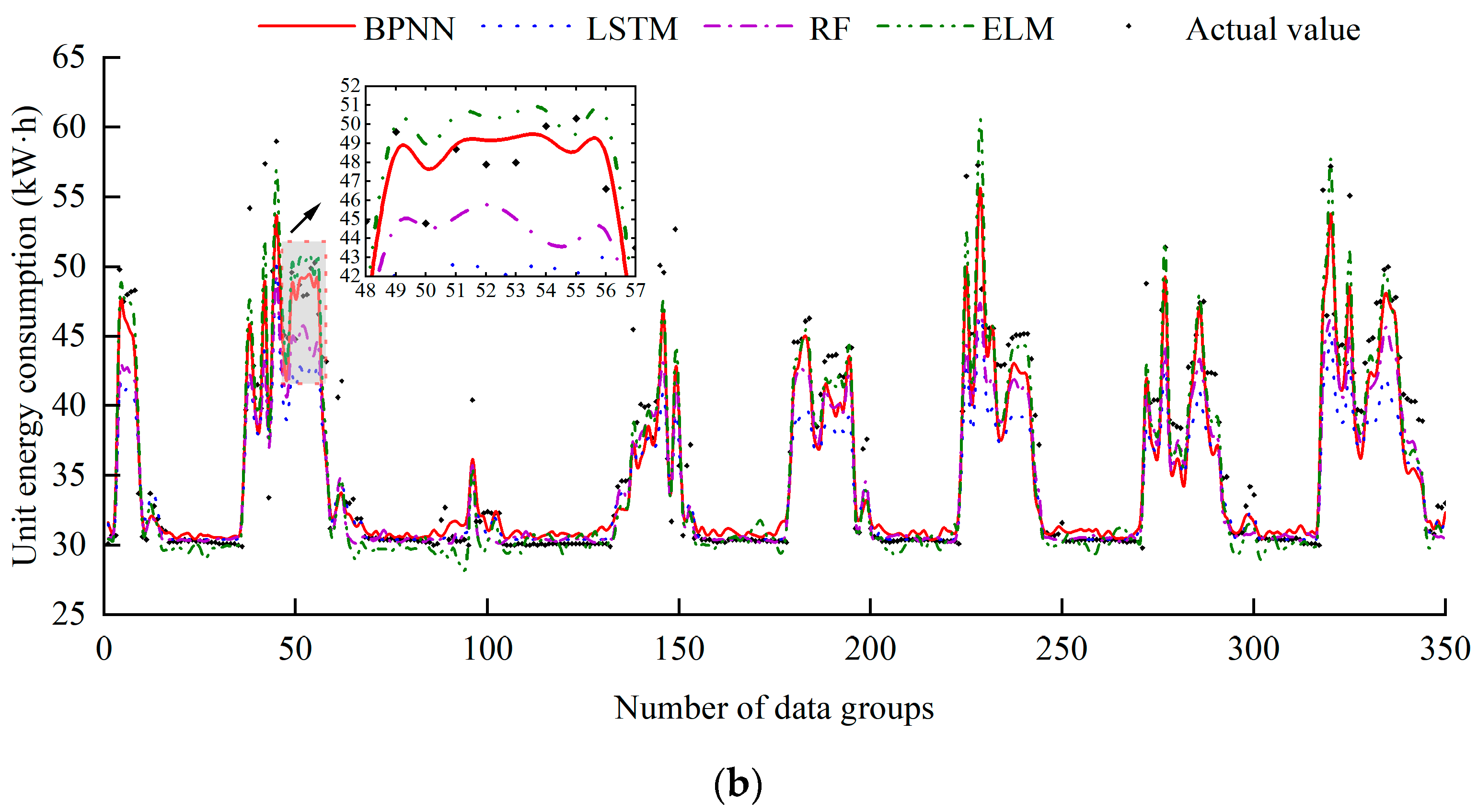
Figure 14 shows the comparison of between the predicted values and actual values for different models. It can be seen that the predicted energy consumptions for the eight models are consistent with the actual values, while minimal differences exist. It can be clearly seen that the MEA-BP model has the highest prediction accuracy, with RMSE, MAE, and MAPE of 1.487 kWh, 0.939 kWh, and 2.429%, respectively. The SVM model then follows, exhibiting metrics that are only slightly higher than those of the MEA-BP model.
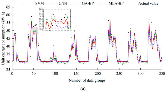
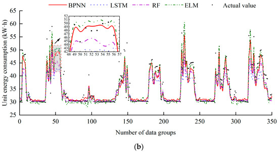
Figure 14.
Comparison between the predicted and actual values for different models: (a) SVM, CNN, GA-BP, MEA-BP and actual value and (b) BPNN, LSTM, RF, ELM and actual value.
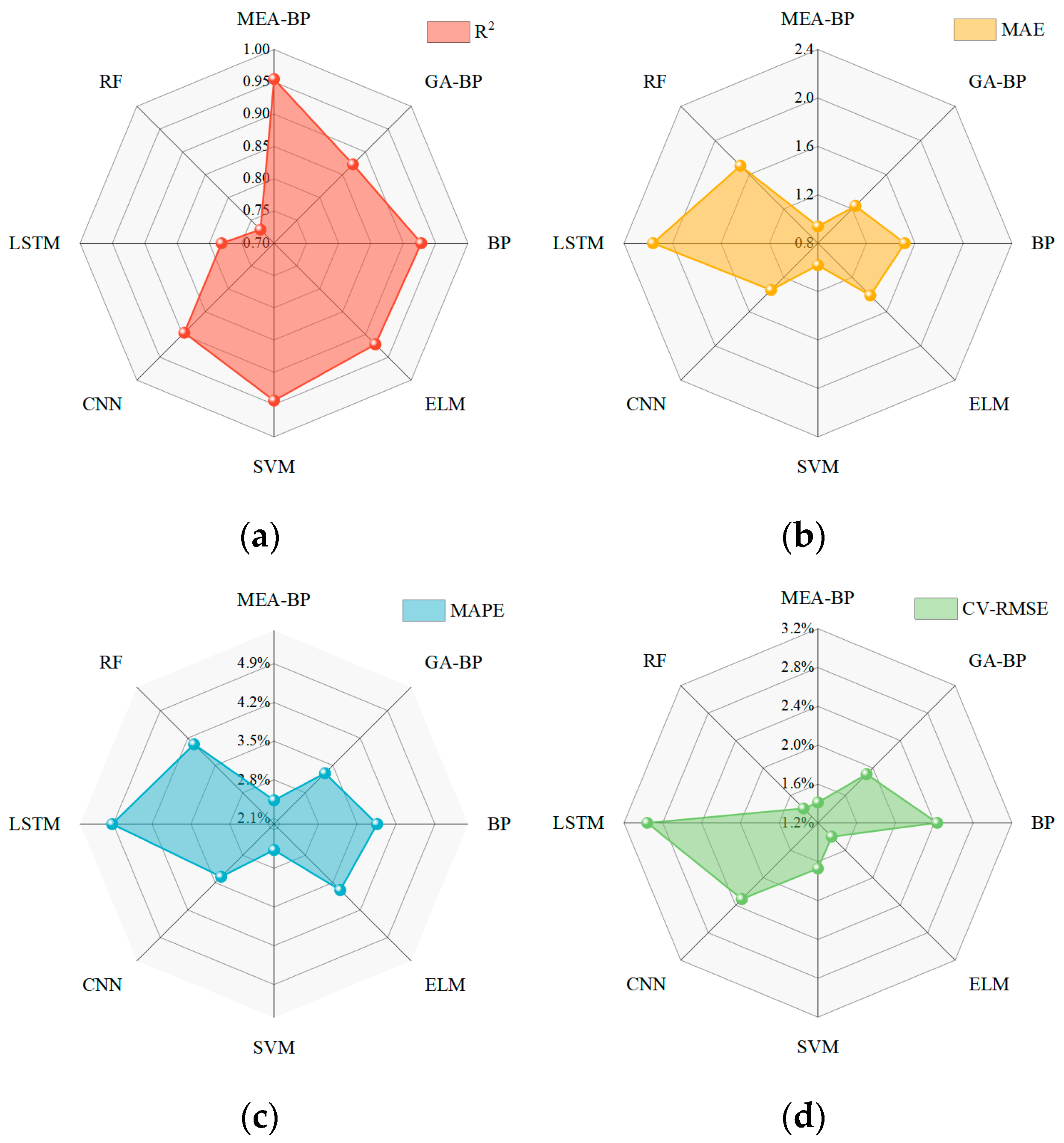
A comprehensive analysis of the R2, MAE, MAPE, and CV-RMSE is presented in Figure 15. It can be seen that all the models have a MAPE and CV-RMSE of less than 10%, demonstrating high performance in the prediction of energy consumption for ground-source heat pump units.
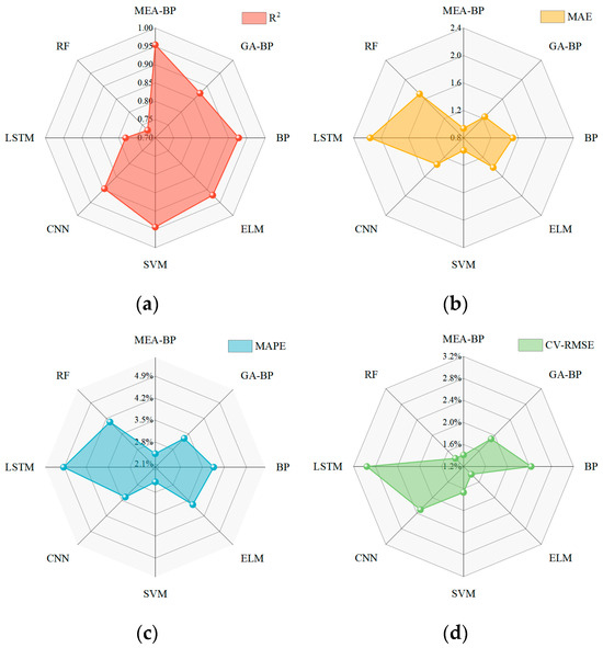
Figure 15.
Comparison between the (a) R2, (b) MAE, (c) MAPE, and (d) CV-RMSE for different models.
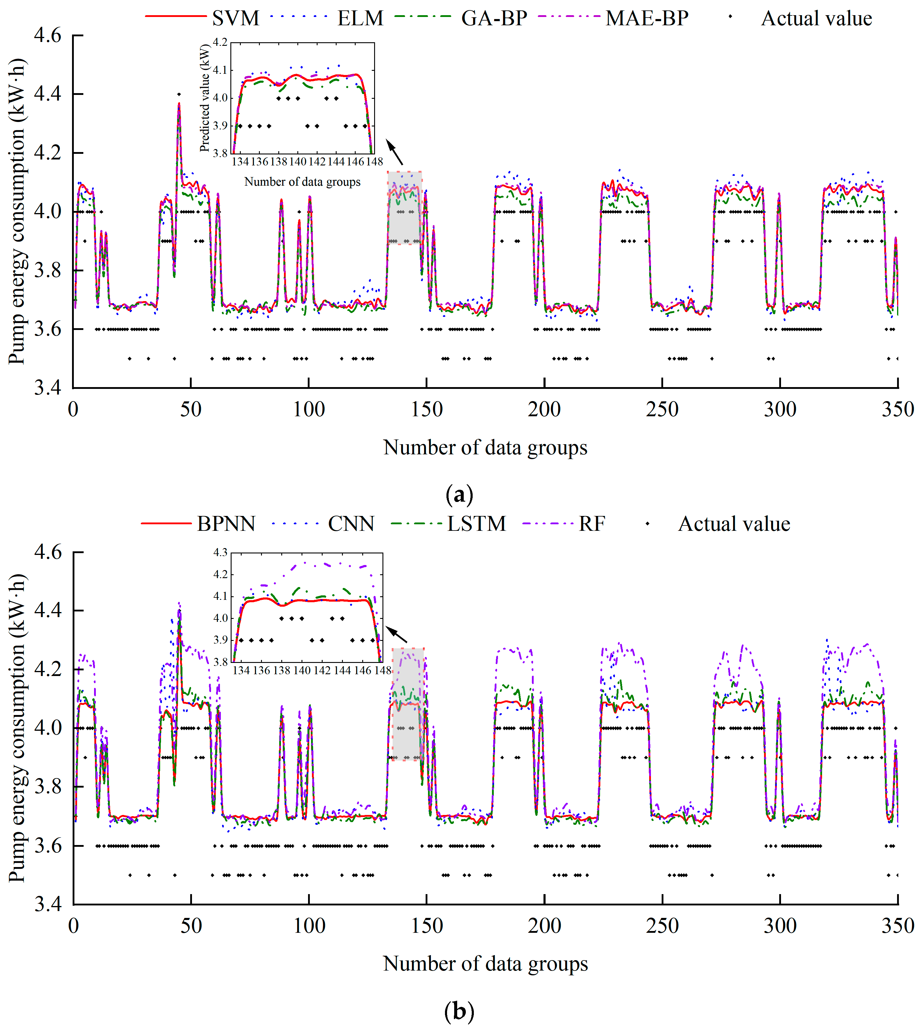
The energy consumption predictions for user pumps obtained by the different models are compared. More precisely, Figure 16 illustrates a comparison between the predicted and actual values for eight different models. It can be clearly seen that the predictions obtained by several models are consistent with the actual values, which indicates a high prediction accuracy.
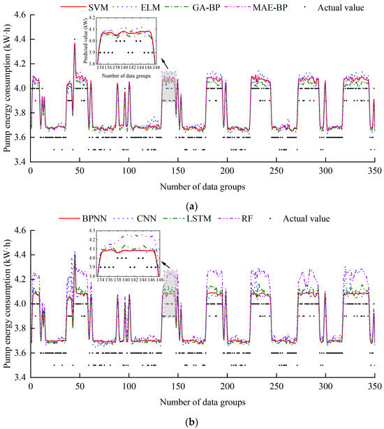
Figure 16.
Comparison between the predicted and actual values for different models: (a) SVM, ELM, GA-BP, MEA-BP and actual value and (b) BPNN, CNN, LSTM, RF and actual value.
Figure 17 shows the comparison between the prediction errors of all the models. It can be seen that the MAEs of all the models are less than 0.2 kW·h, and the MAPEs are less than 5%. This demonstrates that the prediction results have minimal error compared with the actual values, showing high accuracy for all the models. Among the eight models, GA-BP achieves the smallest error, which results in the highest prediction accuracy, reaching R2, MAE, MAPE, and CV-RMSE values of 92.98%, 0.085 kW·h, 2.314%, and 15.53%, respectively. The SVM model then follows, outperforming the MEA-BP model. These results show that the GA-BP model has the highest prediction accuracy for pump energy consumption, while the SVM model also yields satisfactory results. This demonstrates that, under specific conditions, predictions from single models can be consistent with those from composite models, both demonstrating high prediction accuracy.
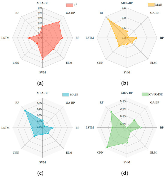
Figure 17.
Comparison between the prediction errors of all the models: (a) R2, (b) MAE, (c) MAPE, and (d) CV-RMSE.
In summary, the MEA-BP model has the highest performance in predicting unit energy consumption, while the GA-BP model achieves the highest accuracy in predicting user pump energy consumption. This demonstrates that under specific conditions, the single models and composite models can perform predictions with high accuracy. However, composite algorithms may yield higher accuracy in certain scenarios. In future work, additional composite algorithms will be incorporated into [46,47].
At present, the control strategies mainly focus on setting the water supply temperature at the ground-source end, while other critical operational parameters, such as the chilled/cooling water flow rates and pump frequency, are neglected. These parameters significantly affect the performance of the air conditioning unit. Therefore, future studies should strive to develop multivariable control strategies that incorporate a broader range of controllable variables to further increase system energy efficiency. In addition, the accuracy of building cooling load predictions is crucial for optimizing the underlying control strategies. The existing studies acknowledge the impact of external environmental factors on cooling loads. However, they often overlook internal factors, such as occupant behavior. To increase the accuracy of the prediction models, future studies should comprehensively consider these factors to better reflect variations in building cooling loads.
Moreover, the existing reinforcement learning algorithms require substantial training data during the control process, leading to a high computational load. To mitigate this complexity and enhance the real-time applicability of control strategies, future studies should explore more efficient optimization algorithms, such as distributed reinforcement learning and online learning. Although the proposed methods achieved very good results in simulation environments, they may encounter some issues in practical engineering applications, such as equipment aging and sensor errors. Therefore, further study is necessary to address potential challenges encountered in real-world applications and to develop appropriate solutions.
The proposed control methods have promising applications in engineering practices, as they can be incorporated into existing HVAC control systems to implement intelligent control strategies. However, these methods cannot completely replace the need for operation and maintenance engineers. Rather, intelligent models can provide engineers with optimal adjustment strategies based on real conditions, which allows for ensuring the stable operation of the systems [19].
Furthermore, due to the intensification of global climate change, extreme temperatures, and seasonal fluctuations may affect the energy efficiency of HVAC systems. Consequently, plans for future studies include conducting comprehensive sensitivity analyses to evaluate the stability and adaptability of the models under varying environmental conditions [19].
In this study, several challenges were encountered. More precisely, during the initial training phase of the DQN, significant fluctuations in reward values were observed. A further analysis demonstrated that this volatility is mainly due to the limitation of the accuracy of the model. Strategic optimization measures, such as regularization techniques and cross-validation, were then implemented to mitigate overfitting risks and to increase the generalization ability of the model. This allows the agent to effectively adapt to prediction model errors during training, which results in increasing the robustness of the control strategies.
In conclusion, the optimization and control of HVAC systems present a challenging yet highly promising field. Due to the advancement of the Internet of Things technologies, accessing various operational data from buildings became feasible. Consequently, leveraging these data to develop data-driven control strategies allows for performing more refined and intelligent HVAC system optimization. Through continuous improvement and in-depth studies, more effective solutions for building energy conservation can be obtained.
6. Conclusions
This study proposes a model-free control method, which integrates reinforcement learning with machine learning predictions, in order to enhance the optimization technology of ground-source heat pump systems. An XGBoost model is developed to forecast cooling load trends, which informs the control decisions of the agent. The effectiveness and robustness of the proposed method are validated through simulation case studies and comparisons with three existing strategies. The obtained results are summarized as follows:
(1) Among the selected models, XGBoost, RF, and LightGBM have R2 values greater than 0.97, with low error evaluation metrics. XGBoost and LightGBM employ boosting tree techniques, underscoring the high potential of this approach in cooling load prediction. The XGBoost model achieves the highest R2 and lowest error indicators, reaching MAPE and CV-RMSE reductions of 80.87% and 53.36%, compared with other prediction models, respectively.
(2) By incorporating reinforcement learning control into machine learning predictions, the deep reinforcement learning regulation approach based on load forecasting has significantly superior energy savings compared with traditional constant water temperature control methods. More precisely, after the algorithm converges, the deep reinforcement learning control method based on load prediction achieves an improvement of 10% in energy savings, compared with conventional methods.
(3) By incorporating predictive information, the deep reinforcement learning regulation method based on load forecasting achieves an average energy savings rate of 8.49%. This denotes an additional efficiency improvement of 0.38% compared with deep reinforcement learning control strategies without predictive information. This enhancement is attributed to the predictive information that allows the agent to better understand future system states, facilitating more rational control decisions.
(4) When only the supply water temperature at the ground source is adjusted, the deep reinforcement learning regulation approach based on load forecasting outperforms empirical formula methods after convergence. In particular, it achieves an energy efficiency improvement of 0.32%. This provides a viable alternative in scenarios with limited data or uncertain equipment conditions. Although the optimization model shows high performance in simulation experiments, it has yet to be validated in actual operating rooms. The adjustment of the model to account for real-world conditions will help its adaptation to genuine environments and optimize system operations.
This study optimizes a ground-source heat pump system and demonstrates the application of deep reinforcement learning in increasing system performance. Deep reinforcement learning provides significant versatility by learning environmental states and action policies, which makes it applicable to the specific system in this case study and to other ground-source heat pump systems. Furthermore, the developed principles and strategies are not limited to ground-source heat pumps. They can also be applied to the optimization and control of general HVAC systems. Therefore, the obtained results have a certain degree of universality, providing valuable insights for the optimization of various air conditioning systems.
Author Contributions
Conceptualization, J.L. and S.L.; data curation, S.L.; formal analysis, J.L.; funding acquisition, J.L.; investigation, Z.W., Y.Q., S.Z., Y.T., X.Z., J.L., and S.L.; methodology, Z.W., S.Z., J.L., and S.L.; project administration, J.L.; software, Z.W., and S.L.; supervision, J.L., and S.L.; validation, S.L.; writing—original draft, Z.W.; writing—review and editing, Y.Q., S.Z., Y.T., X Z., J.L., and S.L. All authors have read and agreed to the published version of the manuscript.
Funding
This work was funded by the National Key Research and Development Program of China (2024YFE0106800) and the Plan of Introduction and Cultivation for Young Innovative Talents in Colleges and Universities of Shandong Province (Lu Jiao Ke Han [2021]. No. 51).
Data Availability Statement
Data are contained within the article.
Conflicts of Interest
Author Zhitao Wang was employed by the company Youshi Technology Development Co., Ltd. Author Yanfa Tian was employed by the company Shandong Huake Planning and Architectural Design Co., Ltd. The remaining authors declare that the research was conducted in the absence of any commercial or financial relationships that could be construed as a potential conflict of interest.
Nomenclature
| CL | cooling load, kW |
| SR | solar radiation, W/m2 |
| Tout | outdoor temperature, °C |
| v | outdoor wind speed, m/s |
| α | wind direction, ° |
| φ | relative humidity, % |
| Abbreviation | |
| A | action |
| BPNN | back propagation neural network |
| CNN | convolutional neural network |
| CV-RMSE | coefficient of variation in the root mean squared error |
| DRL | deep reinforcement learning |
| ELM | extreme learning machine |
| GA-BP | genetic algorithm-based back propagation neural network |
| HVAC | heating, ventilation, and air conditioning |
| LightGBM | light gradient boosting machine |
| LSTM | long short-term memory |
| MAE | mean absolute error |
| MAPE | mean absolute percentage error |
| MDP | markov decision process |
| MEA-BP | mind evolutionary algorithm-based back propagation neural network |
| P | transition probability |
| R | reward |
| R2 | coefficient of determination |
| RBFN | radial basis function network |
| RF | random forest |
| RL | reinforcement Learning |
| RMSE | root mean squared error |
| S | state |
| SVM | support vector machine |
| XGBoost | extreme gradient boosting |
| γ | discount factor |
References
- Gorzałczany, M.B.; Rudziński, F. Energy Consumption Prediction in Residential Buildings—An Accurate and Interpretable Machine Learning Approach Combining Fuzzy Systems with Evolutionary Optimization. Energies 2024, 17, 3242. [Google Scholar] [CrossRef]
- Shi, Z.; Zheng, R.; Shen, R.; Yang, D.; Wang, G.; Liu, Y.; Li, Y.; Zhao, J. Building heating load forecasting based on the theory of transient heat transfer and deep learning. Energy Build. 2024, 313, 114290. [Google Scholar] [CrossRef]
- Cui, M.; Liu, J.; Kim, M.K.; Wu, X. Application potential analysis of different control strategies for radiant floor cooling systems in office buildings in different climate zones of China. Energy Build. 2023, 282, 112772. [Google Scholar] [CrossRef]
- Homod, R.Z.; Mohammed, H.I.; Ben Hamida, M.B.; Albahri, A.S.; Alhasnawi, B.N.; Albahri, O.S.; Alamoodi, A.H.; Mahdi, J.M.; Albadr, M.A.A.; Yaseen, Z.M. Optimal shifting of peak load in smart buildings using multiagent deep clustering reinforcement learning in multi-tank chilled water systems. J. Energy Storage 2024, 92, 112140. [Google Scholar] [CrossRef]
- Kim, Y.-S.; Kim, M.K.; Fu, N.; Liu, J.; Wang, J.; Srebric, J. Investigating the Impact of Data Normalization Methods on Predicting Electricity Consumption in a Building Using different Artificial Neural Network Models. Sustain. Cities Soc. 2025, 118, 105570. [Google Scholar] [CrossRef]
- Sun, L.; Hu, Z.; Mae, M.; Imaizumi, T. Individual room air-conditioning control in high-insulation residential building during winter: A deep reinforcement learning-based control model for reducing energy consumption. Energy Build. 2024, 323, 114799. [Google Scholar] [CrossRef]
- He, K.; Fu, Q.; Lu, Y.; Ma, J.; Zheng, Y.; Wang, Y.; Chen, J. Efficient model-free control of chiller plants via cluster-based deep reinforcement learning. J. Build. Eng. 2024, 82, 108345. [Google Scholar] [CrossRef]
- Su, Y.; Zou, X.; Tan, M.; Peng, H.; Chen, J. Integrating few-shot personalized thermal comfort model and reinforcement learning for HVAC demand response optimization. J. Build. Eng. 2024, 91, 109509. [Google Scholar] [CrossRef]
- Fu, Q.; Chen, X.; Ma, S.; Fang, N.; Xing, B.; Chen, J. Optimal control method of HVAC based on multi-agent deep reinforcement learning. Energy Build. 2022, 270, 112284. [Google Scholar] [CrossRef]
- Gupta, A.; Badr, Y.; Negahban, A.; Qiu, R.G. Energy-efficient heating control for smart buildings with deep reinforcement learning. J. Build. Eng. 2021, 34, 101739. [Google Scholar] [CrossRef]
- Du, Y.; Li, F.; Munk, J.; Kurte, K.; Kotevska, O.; Amasyali, K.; Zandi, H. Multi-task deep reinforcement learning for intelligent multi-zone residential HVAC control. Electr. Power Syst. Res. 2021, 192, 106959. [Google Scholar] [CrossRef]
- Deng, Z.; Chen, Q. Reinforcement learning of occupant behavior model for cross-building transfer learning to various HVAC control systems. Energy Build. 2021, 238, 110860. [Google Scholar] [CrossRef]
- Jiang, Z.; Risbeck, M.J.; Ramamurti, V.; Murugesan, S.; Amores, J.; Zhang, C.; Lee, Y.M.; Drees, K.H. Building HVAC control with reinforcement learning for reduction of energy cost and demand charge. Energy Build. 2021, 239, 110833. [Google Scholar] [CrossRef]
- Zou, Z.; Yu, X.; Ergan, S. Towards optimal control of air handling units using deep reinforcement learning and recurrent neural network. Build. Environ. 2020, 168, 106535. [Google Scholar] [CrossRef]
- Qiu, S.; Li, Z.; Li, Z.; Li, J.; Long, S.; Li, X. Model-free control method based on reinforcement learning for building cooling water systems: Validation by measured data-based simulation. Energy Build. 2020, 218, 110055. [Google Scholar] [CrossRef]
- Moayedi, H.; Mukhtar, A.; Khedher, N.B.; Elbadawi, I.; Amara, M.B.; Tt, Q.; Khalilpoor, N. Forecasting of energy-related carbon dioxide emission using ANN combined with hybrid metaheuristic optimization algorithms. Eng. Appl. Comput. Fluid Mech. 2024, 18, 2322509. [Google Scholar] [CrossRef]
- Khedher, N.B.; Mukhtar, A.; Md Yasir, A.S.H.; Khalilpoor, N.; Foong, L.K.; Nguyen Le, B.; Yildizhan, H. Approximating heat loss in smart buildings through large scale experimental and computational intelligence solutions. Eng. Appl. Comput. Fluid Mech. 2023, 17, 2226725. [Google Scholar] [CrossRef]
- Khan, M.I.; Ghodhbani, R.; Taha, T.; Al-Yarimi, F.A.M.; Zeeshan, A.; Ijaz, N.; Khedher, N.B. Advanced intelligent computing ANN for momentum, thermal, and concentration boundary layers in plasma electro hydrodynamics burgers fluid. Int. Commun. Heat Mass Transf. 2024, 159, 108195. [Google Scholar] [CrossRef]
- Lu, S.; Zhou, S.; Ding, Y.; Kim, M.K.; Yang, B.; Tian, Z.; Liu, J. Exploring the comprehensive integration of artificial intelligence in optimizing HVAC system operations: A review and future outlook. Results Eng. 2025, 25, 103765. [Google Scholar] [CrossRef]
- Liu, X.; Gou, Z. Occupant-centric HVAC and window control: A reinforcement learning model for enhancing indoor thermal comfort and energy efficiency. Build. Environ. 2024, 250, 111197. [Google Scholar] [CrossRef]
- Corriou, J.-P. Dynamic Optimization. In Numerical Methods and Optimization: Theory and Practice for Engineers; Springer International Publishing: Cham, Switzerland, 2021; pp. 653–708. [Google Scholar]
- Homod, R.Z.; Yaseen, Z.M.; Hussein, A.K.; Almusaed, A.; Alawi, O.A.; Falah, M.W.; Abdelrazek, A.H.; Ahmed, W.; Eltaweel, M. Deep clustering of cooperative multi-agent reinforcement learning to optimize multi chiller HVAC systems for smart buildings energy management. J. Build. Eng. 2023, 65, 105689. [Google Scholar] [CrossRef]
- Chen, B.; Zeng, W.; Nie, H.; Deng, Z.; Yang, W.; Yan, B. Optimal load distribution control for airport terminal chiller units based on deep reinforcement learning. J. Build. Eng. 2024, 97, 110787. [Google Scholar] [CrossRef]
- Borja-Conde, J.A.; Nadales, J.M.; Ordonez, J.G.; Fele, F.; Limon, D. Efficient management of HVAC systems through coordinated operation of parallel chiller units: An economic predictive control approach. Energy Build. 2024, 304, 113879. [Google Scholar] [CrossRef]
- Sun, M.; Yang, J.; Yang, C.; Wang, W.; Wang, X.; Li, H. Research on prediction of PPV in open-pit mine used RUN-XGBoost model. Heliyon 2024, 10, e28246. [Google Scholar] [CrossRef] [PubMed]
- Wang, H.; Chen, Y.; Kang, J.; Ding, Z.; Zhu, H. An XGBoost-Based predictive control strategy for HVAC systems in providing day-ahead demand response. Build. Environ. 2023, 238, 110350. [Google Scholar] [CrossRef]
- Seyyedattar, M.; Zendehboudi, S.; Ghamartale, A.; Afshar, M. Advancing hydrogen storage predictions in metal-organic frameworks: A comparative study of LightGBM and random forest models with data enhancement. Int. J. Hydrogen Energy 2024, 69, 158–172. [Google Scholar] [CrossRef]
- Aparicio-Ruiz, P.; Barbadilla-Martín, E.; Guadix, J.; Nevado, J. Analysis of Variables Affecting Indoor Thermal Comfort in Mediterranean Climates Using Machine Learning. Buildings 2023, 13, 2215. [Google Scholar] [CrossRef]
- Hou, X.; Guo, X.; Yuan, Y.; Zhao, K.; Tong, L.; Yuan, C.; Teng, L. The state of health prediction of Li-ion batteries based on an improved extreme learning machine. J. Energy Storage 2023, 70, 108044. [Google Scholar] [CrossRef]
- Lei, L.; Shao, S. Prediction model of the large commercial building cooling loads based on rough set and deep extreme learning machine. J. Build. Eng. 2023, 80, 107958. [Google Scholar] [CrossRef]
- Wang, Q.; Qi, J.; Hosseini, S.; Rasekh, H.; Huang, J. ICA-LightGBM Algorithm for Predicting Compressive Strength of Geo-Polymer Concrete. Buildings 2023, 13, 2278. [Google Scholar] [CrossRef]
- Ni, C.; Huang, H.; Cui, P.; Ke, Q.; Tan, S.; Ooi, K.T.; Liu, Z. Light Gradient Boosting Machine (LightGBM) to forecasting data and assisting the defrosting strategy design of refrigerators. Int. J. Refrig. 2024, 160, 182–196. [Google Scholar] [CrossRef]
- Zheng, G.; Feng, Z.; Jiang, M.; Tan, L.; Wang, Z. Predicting the Energy Consumption of Commercial Buildings Based on Deep Forest Model and Its Interpretability. Buildings 2023, 13, 2162. [Google Scholar] [CrossRef]
- An, W.; Zhu, X.; Yang, K.; Kim, M.K.; Liu, J. Hourly Heat Load Prediction for Residential Buildings Based on Multiple Combination Models: A Comparative Study. Buildings 2023, 13, 2340. [Google Scholar] [CrossRef]
- Pastre, G.G.; Balbinot, A.; Pedroni, R. Virtual temperature sensor using Support Vector Machines for autonomous uninterrupted automotive HVAC systems control. Int. J. Refrig. 2022, 144, 128–135. [Google Scholar] [CrossRef]
- He, K.; Fu, Q.; Lu, Y.; Wang, Y.; Luo, J.; Wu, H.; Chen, J. Predictive control optimization of chiller plants based on deep reinforcement learning. J. Build. Eng. 2023, 76, 107158. [Google Scholar] [CrossRef]
- An, W.; Gao, B.; Liu, J.; Ni, J.; Liu, J. Predicting hourly heating load in residential buildings using a hybrid SSA–CNN–SVM approach. Case Stud. Therm. Eng. 2024, 59, 104516. [Google Scholar] [CrossRef]
- Ajifowowe, I.; Chang, H.; Lee, C.S.; Chang, S. Prospects and challenges of reinforcement learning-based HVAC control. J. Build. Eng. 2024, 98, 111080. [Google Scholar] [CrossRef]
- Lu, S.; Cui, M.; Gao, B.; Liu, J.; Ni, J.; Liu, J.; Zhou, S. A Comparative Analysis of Machine Learning Algorithms in Predicting the Performance of a Combined Radiant Floor and Fan Coil Cooling System. Buildings 2024, 14, 1659. [Google Scholar] [CrossRef]
- Wen, H.; Liu, B.; Di, M.; Li, J.; Zhou, X. A SHAP-enhanced XGBoost model for interpretable prediction of coseismic landslides. Adv. Space Res. 2024, 74, 3826–3854. [Google Scholar] [CrossRef]
- Sun, Z.; Wang, X.; Huang, H.; Yang, Y.; Wu, Z. Predicting compressive strength of fiber-reinforced coral aggregate concrete: Interpretable optimized XGBoost model and experimental validation. Structures 2024, 64, 106516. [Google Scholar] [CrossRef]
- Hu, J. Prediction of the internal corrosion rate for oil and gas pipelines and influence factor analysis with interpretable ensemble learning. Int. J. Press. Vessel. Pip. 2024, 212, 105329. [Google Scholar] [CrossRef]
- Keun Kim, M.; Cremers, B.; Fu, N.; Liu, J. Predictive and correlational analysis of heating energy consumption in four residential apartments with sensitivity analysis using long Short-Term memory and Generalized regression neural network models. Sustain. Energy Technol. Assess. 2024, 71, 103976. [Google Scholar] [CrossRef]
- Zhang, C.; Ma, L.; Han, X.; Zhao, T. Reconstituted data-driven air conditioning energy consumption prediction system employing occupant-orientated probability model as input and swarm intelligence optimization algorithms. Energy 2024, 288, 129799. [Google Scholar] [CrossRef]
- Zhang, C.; Luo, Z.; Rezgui, Y.; Zhao, T. Enhancing multi-scenario data-driven energy consumption prediction in campus buildings by selecting appropriate inputs and improving algorithms with attention mechanisms. Energy Build. 2024, 311, 114133. [Google Scholar] [CrossRef]
- Xu, M.; Liu, W.; Wang, S.; Tian, J.; Wu, P.; Xie, C. A 24-Step Short-Term Power Load Forecasting Model Utilizing KOA-BiTCN-BiGRU-Attentions. Energies 2024, 17, 4742. [Google Scholar] [CrossRef]
- Guenoukpati, A.; Agbessi, A.P.; Salami, A.A.; Bakpo, Y.A. Hybrid Long Short-Term Memory Wavelet Transform Models for Short-Term Electricity Load Forecasting. Energies 2024, 17, 4914. [Google Scholar] [CrossRef]


Disclaimer/Publisher’s Note: The statements, opinions and data contained in all publications are solely those of the individual author(s) and contributor(s) and not of MDPI and/or the editor(s). MDPI and/or the editor(s) disclaim responsibility for any injury to people or property resulting from any ideas, methods, instructions or products referred to in the content. |
© 2025 by the authors. Licensee MDPI, Basel, Switzerland. This article is an open access article distributed under the terms and conditions of the Creative Commons Attribution (CC BY) license (https://creativecommons.org/licenses/by/4.0/).