Article

Upsampling Monte Carlo Reactor Simulation Tallies in Depleted Sodium-Cooled Fast Reactor Assemblies Using a Convolutional Neural Network

1
Nuclear Science & Engineering, The Colorado School of Mines, 1012 14th St., Golden, CO 80401, USA
2
Argonne National Laboratory, 9700 S Cass Avenue, Lemont, IL 60439, USA
3
Department of Mechanical Engineering, The Colorado School of Mines, 1610 Illinois St., Golden, CO 80401, USA
*
Author to whom correspondence should be addressed.
Energies 2024, 17(9), 2177; https://doi.org/10.3390/en17092177
Submission received: 28 March 2024 / Revised: 20 April 2024 / Accepted: 26 April 2024 / Published: 2 May 2024
(This article belongs to the Section B4: Nuclear Energy)

Abstract

:
The computational demand of neutron Monte Carlo transport simulations can increase rapidly with the spatial and energy resolution of tallied physical quantities. Convolutional neural networks have been used to increase the resolution of Monte Carlo simulations of light water reactor assemblies while preserving accuracy with negligible additional computational cost. Here, we show that a convolutional neural network can also be used to upsample tally results from Monte Carlo simulations of sodium-cooled fast reactor assemblies, thereby extending the applicability beyond thermal systems. The convolutional neural network model is trained using neutron flux tallies from 300 procedurally generated nuclear reactor assemblies simulated using OpenMC. Validation and test datasets included 16 simulations of procedurally generated assemblies, and a realistic simulation of a European sodium-cooled fast reactor assembly was included in the test dataset. We show the residuals between the high-resolution flux tallies predicted by the neural network and high-resolution Monte Carlo tallies on relative and absolute bases. The network can upsample tallies from simulations of fast reactor assemblies with diverse and heterogeneous materials and geometries by a factor of two in each spatial and energy dimension. The network’s predictions are within the statistical uncertainty of the Monte Carlo tallies in almost all cases. This includes test assemblies for which burnup values and geometric parameters were well outside the ranges of those in assemblies used to train the network.

1. Introduction

The significant computational demand associated with high-resolution Monte Carlo simulations of nuclear reactor cores has motivated the development of CPU and memory-efficient methods to increase the simulations’ fidelity. Monte Carlo codes, such as Serpent [1], OpenMC [2], and MCNP [3], implement a variety of such methods, including Functional Expansion Tallies (FETs) [4] and domain decomposition. FETs can increase the resolution of neutron flux tallies by expanding the spatial and angle-dependent neutron flux using orthogonal functions. Methods based on domain decomposition divide the workload of a single compute node among several parallel nodes. This method is useful when the simulation is too large to fit in memory and has been implemented in Serpent, as well as in a developmental version of OpenMC [5,6]. Disjoint tallies have a basis in compressed sensing methods and have also been shown to yield significant memory reductions in neutron Monte Carlo simulations [7,8].
Machine learning approaches have also been used to increase neutron flux tallies’ spatial and energy resolution without any significant increase in CPU or memory requirements. Convolutional neural networks (CNNs) were used in [9,10] to upsample Monte Carlo neutron flux tallies in simulations of light water reactor (LWR) assemblies. The low-resolution tallies were calculated at a spatial resolution of 64 × 64 pixels and with eight neutron energy groups and were upsampled to 128 × 128 pixels and 16 groups. Although the CNNs were able to upsample LWR tallies accurately over a diverse range of assembly geometries, fuel enrichment, and burnup levels, their applicability to fast reactors was not established. Here, we show that a CNN can be used to upsample neutron flux tallies from Monte Carlo simulations of sodium-cooled fast reactor (SFR) assemblies. We constrained the training data to heterogeneous hexagonal assemblies with one to five rings of pins and with fuel burned up to 180 MWd/kgIHM. Fuel isotopics in the training data were taken from depletion simulations of LWR assemblies fueled with uranium dioxide enriched to 1.6%, as well as fresh fuel. The fresh-fueled assemblies in the training data included uranium dioxide (UOX) and pure uranium metal enriched to 11%. To increase the diversity of the training data, we also included samples with thermal spectra and training samples with boron-shielded fuel and no coolant that produced very hard spectra. The validation data consisted of SFR assemblies with 10 and 11 rings of pins and fuel with burnup levels of up to 180 MWd/kgIHM. The test data included SFR assemblies with 10 and 11 rings of pins and fuel with burnup levels of up to 400 MWd/kgIHM. Fuel isotopics in the test and validation data originate from depletion simulations of LWR assemblies with UOX enriched to 1.6% and 19.9%, as well as fresh fuel. Fuel in the testing and validation data included UOX, mixed-oxide (MOX), and uranium–plutonium–zirconium (UPuZr) alloys. All assemblies in the training and validation datasets were generated by randomly selecting geometry, temperatures, and materials using Latin hypercube sampling. This was also done to generate the test data, although this dataset also included a realistic assembly simulation of the European sodium-cooled fast reactor (ESFR) [11].
The CNN topology was the same as in [10], which included three residual blocks and a 3 × 3 kernel in all convolutional layers. The CNN in this work, however, featured 256 filters in each convolutional layer and exponential linear unit (ELU) activations. Inputs to the CNN and ground truth quantities used to calculate the loss were low- and high-resolution flux tallies, respectively, computed using OpenMC. The accuracy of the CNN was shown by comparing the residuals between the predictions and ground truth with the standard deviation in the ground truth tallies computed using OpenMC. We also calculated the fraction of predictions made by the CNN that lie outside one and two standard deviations of the ground truth. We found that a residual CNN can increase the resolution of 2-D neutron flux tallies in simulated SFR assemblies by a factor of two in the spatial and energy dimensions. The accuracy of the upsampled neutron flux tallies calculated using the CNN was comparable to the uncertainty in the tallies computed using high-resolution Monte Carlo simulations.

2. Methods

2.1. Data Generation

All datasets consisted of neutron flux mesh tallies and their uncertainties at low and high resolutions generated using the OpenMC Monte Carlo code [2] and ENDF/B-VIII.0 [12] nuclear data. The spatial resolution of the low- and high-resolution tallies was 0.1 × 0.1 cm and 0.05 × 0.05 cm, respectively. The energy grids of the low- and high-resolution tallies consisted of 8 and 16 groups, respectively, with group boundaries in equal logarithmic spacing between 100 eV and 20 MeV. Criticality eigenvalue simulations used 50 inactive cycles, 100 active cycles, and 100,000 source neutrons per cycle. Input decks for OpenMC were created using the OpenMC Python API and an in-house Python code [13]. The Python code used Latin hypercube sampling to select the geometry and materials of the assembly and individual fuel pins according to specified ranges and choices. Individual fuel pin parameters that could be randomly selected were fuel radius, temperature and burnup level, and cladding thickness. The sampling method could also randomly select B4C or sodium for the contents of the pin. The randomly chosen assembly parameters included coolant temperature, duct thickness, and the number of rings of pins. The ranges of all geometric parameters used in the generation of training, validation, and testing datasets are given in Table 1.
The training datasets were compiled from simulations of assemblies with 2 to 5 rings of pins and fuel burnup levels ranging from 0 to 180 MWd/kgIHM. Validation and testing datasets were compiled from simulations of assemblies with 10 or 11 rings of pins and fuel burnup levels of up to 400 MWd/kgIHM. These values in the validation and test datasets were chosen to show that the CNN could make accurate predictions in assemblies with geometry and burnup well beyond those in the training data. The test dataset also contained a simulation of an ESFR assembly to show that the CNN could accurately upsample simulations of assembly models with realistic geometries and materials. The geometry of the selected representative sample assemblies from the training data and validation/test data are shown in Figure 1.
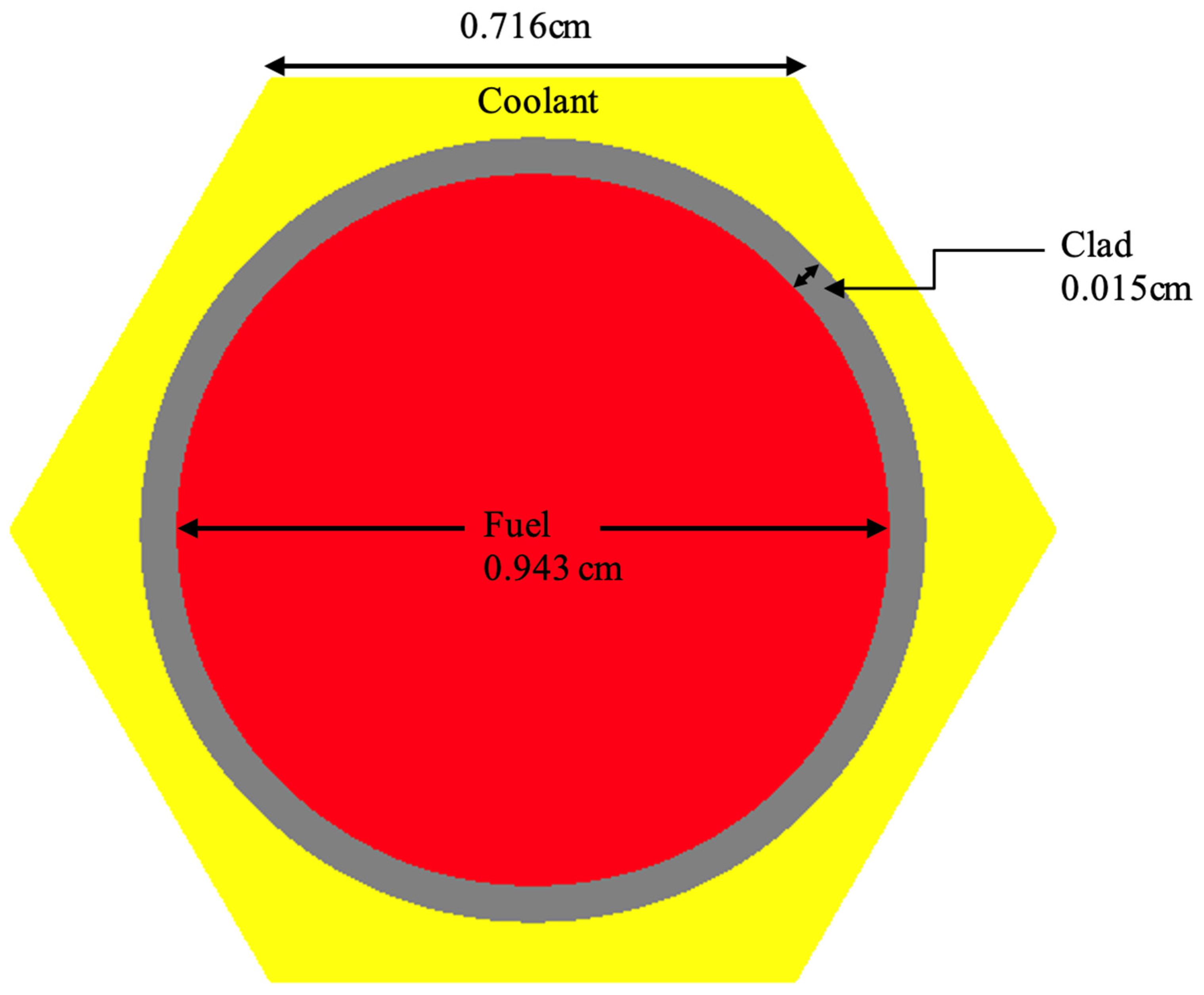
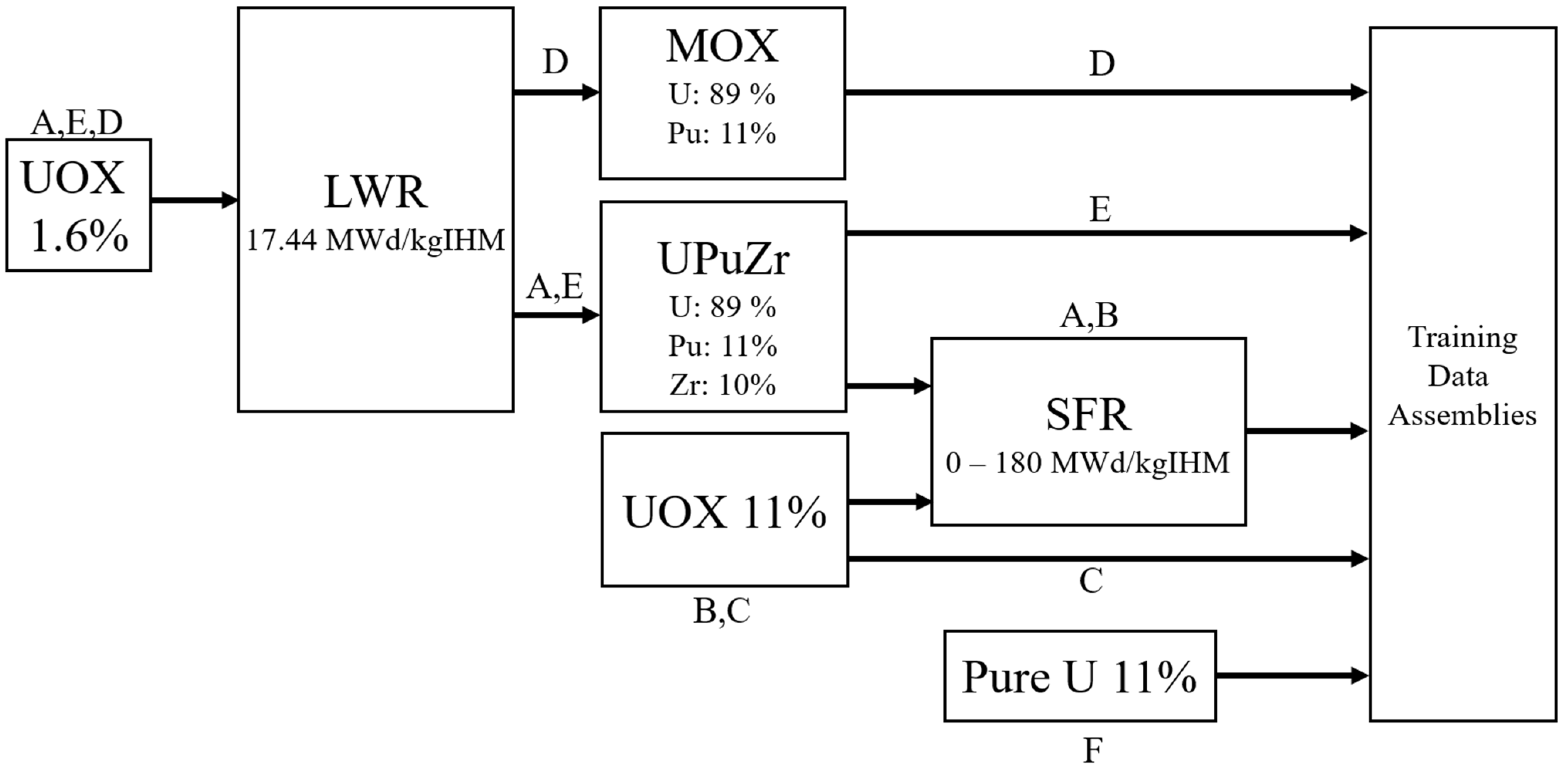
The assemblies in all datasets contained a mix of UPuZr, UOX, MOX, and pure metal uranium fuel. Table 2 summarizes the main characteristics of the training (A-F), validation (G-J), and test (K-O) datasets. The fuel isotopics in all datasets containing depleted assemblies (A, B, G-J, L-O) were determined using SFR pincell burnup simulations performed in OpenMC. Figure 2 shows the geometry used in the SFR pincell burnup simulations. Training datasets A, E, and D contained either UPuZr or MOX fuel with plutonium isotopics originating from UOX enriched to 1.6% and burned to 17.44 MWd/kgIHM in an LWR. The LWR depletion simulations had been performed previously in [10]. Training dataset B contained UOX enriched to 11% and burned up to 180 MWd/kgIHM in the SFR pincell depletion simulations. Training datasets C and F contained fresh UOX and fresh pure U, respectively, enriched to 11% in both cases. Figure 3 shows a flow diagram indicating the origin of all fuel types used in each training dataset.
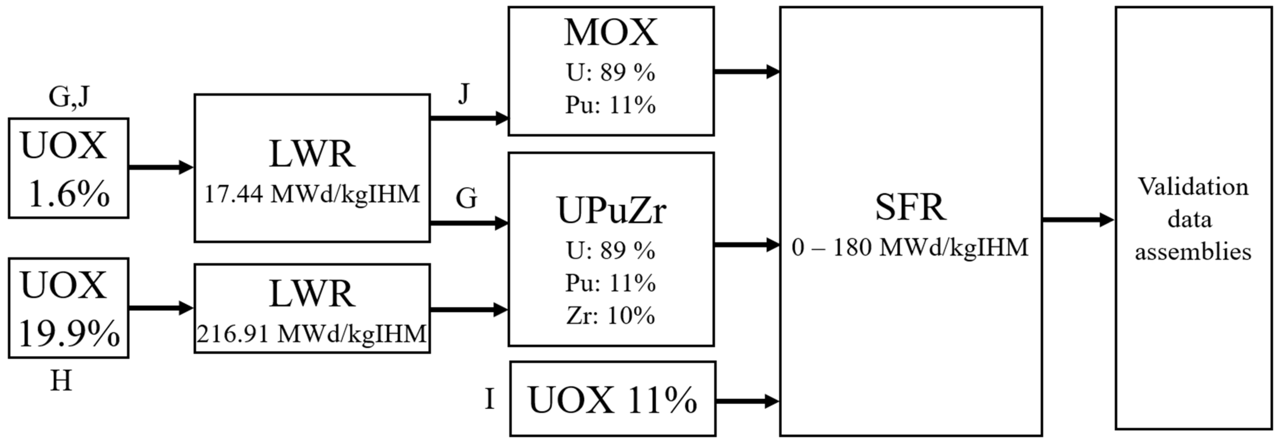
Validation datasets G, H, and J contained either UPuZr or MOX fuel with plutonium isotopics originating from UOX burned in an LWR. In datasets G and J, the UOX was enriched to 1.6% and burned to 17.44 MWd/kgIHM. In the case of dataset H, the UOX was enriched to 19.9% and burned to 216.91 MWd/kgIHM. Validation dataset I contained UOX enriched to 11%. All MOX, UPuZr, and UOX fuels were then burned in SFR pincell depletion simulations up to 180 MWd/kgIHM before being used in assembly simulations. Figure 4 shows a flow diagram indicating the origin of all fuel types used in each validation dataset.
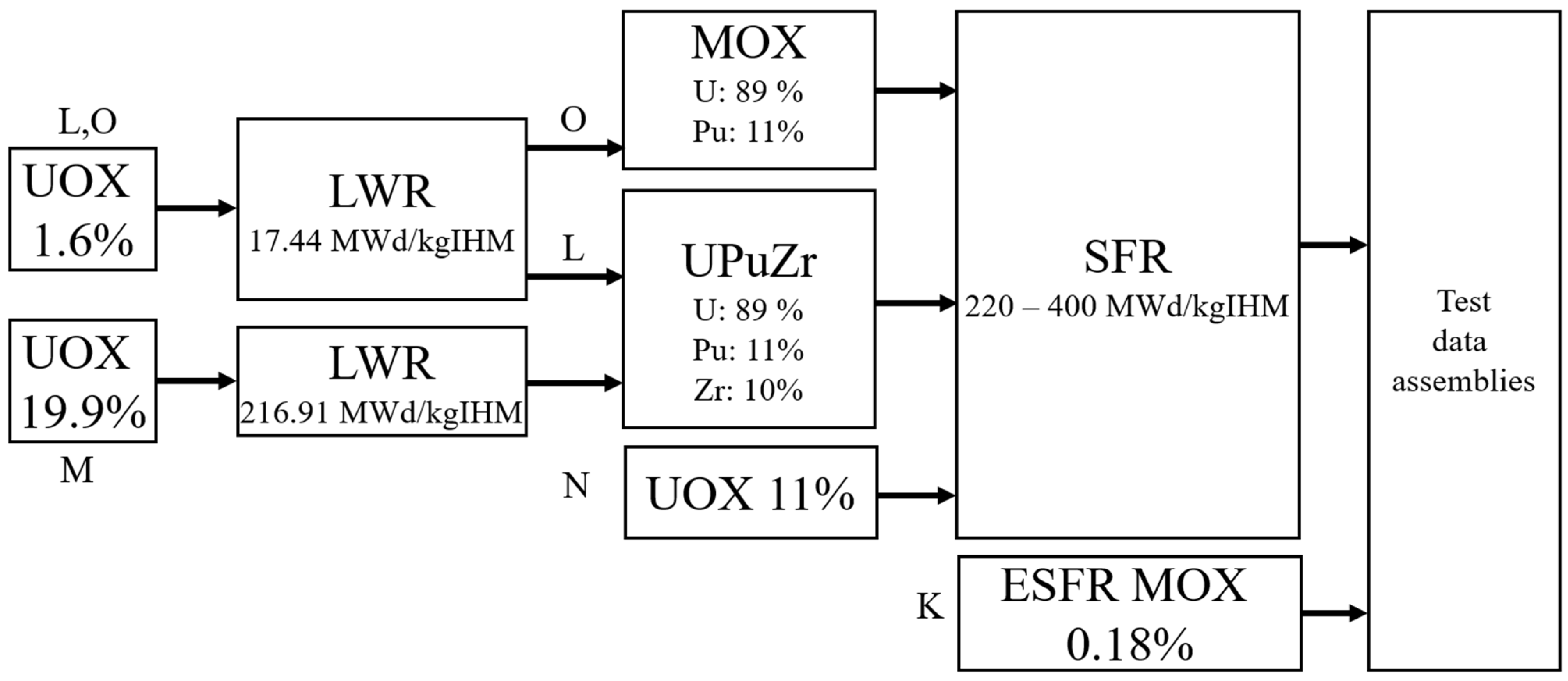
Test datasets M, N, and O contained either UPuZr or MOX fuel with plutonium isotopics originating from UOX burned in an LWR. In datasets L and O, the UOX was enriched to 1.6% and burned to 17.44 MWd/kgIHM. In dataset M, the UOX was enriched to 19.9% and burned to 216.91 MWd/kgIHM. Test dataset N contained UOX enriched to 11%. All MOX, UPuZr, and UOX fuels in test datasets L, M, N, and O were then burned in SFR pincell depletion simulations from 220 to 400 MWd/kgIHM before being used in assembly simulations. Test dataset K contained MOX fuel with isotopics from the ESFR reactor [11]. Figure 5 shows a flow diagram indicating the origin of all fuel types used in each test dataset.
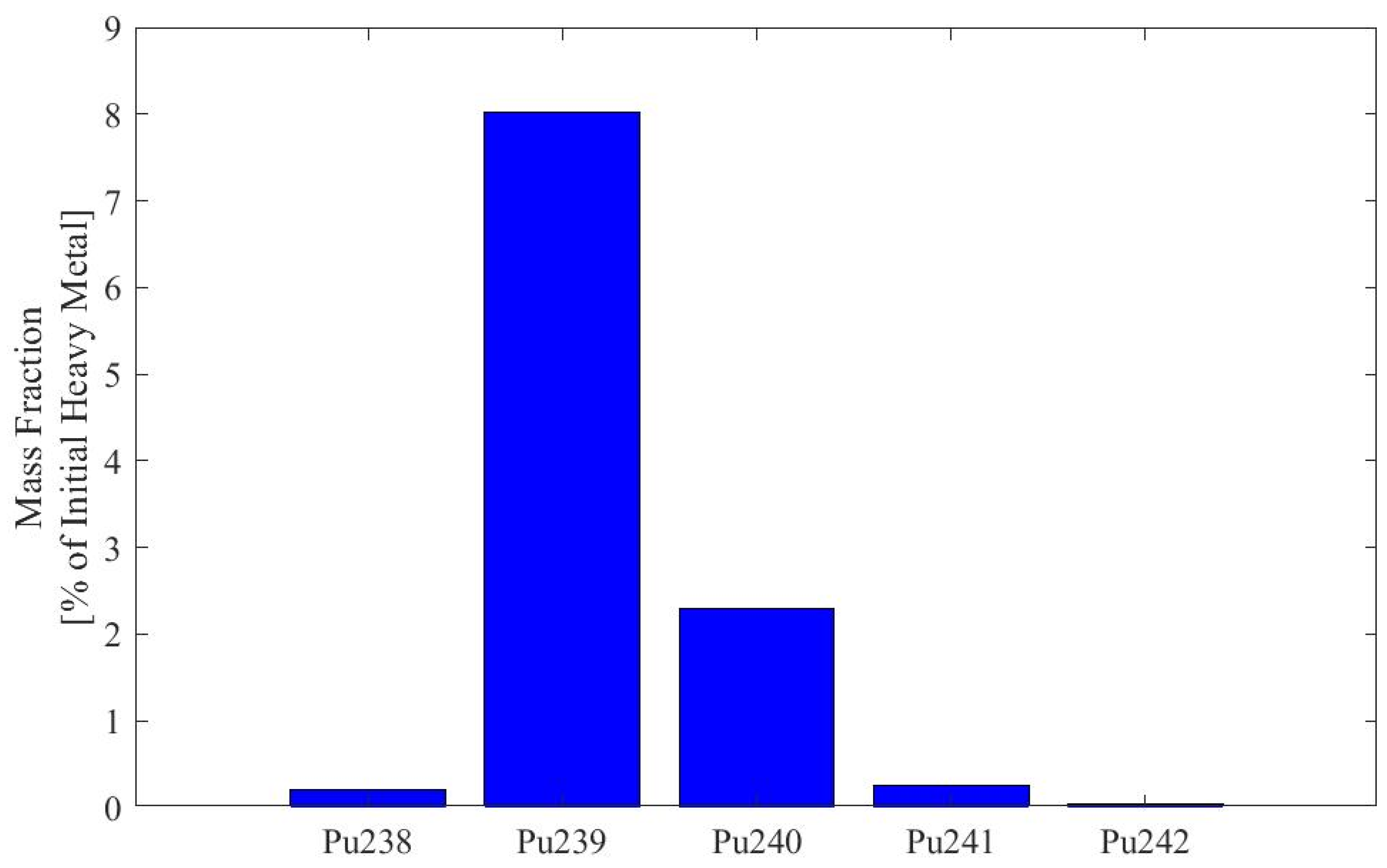
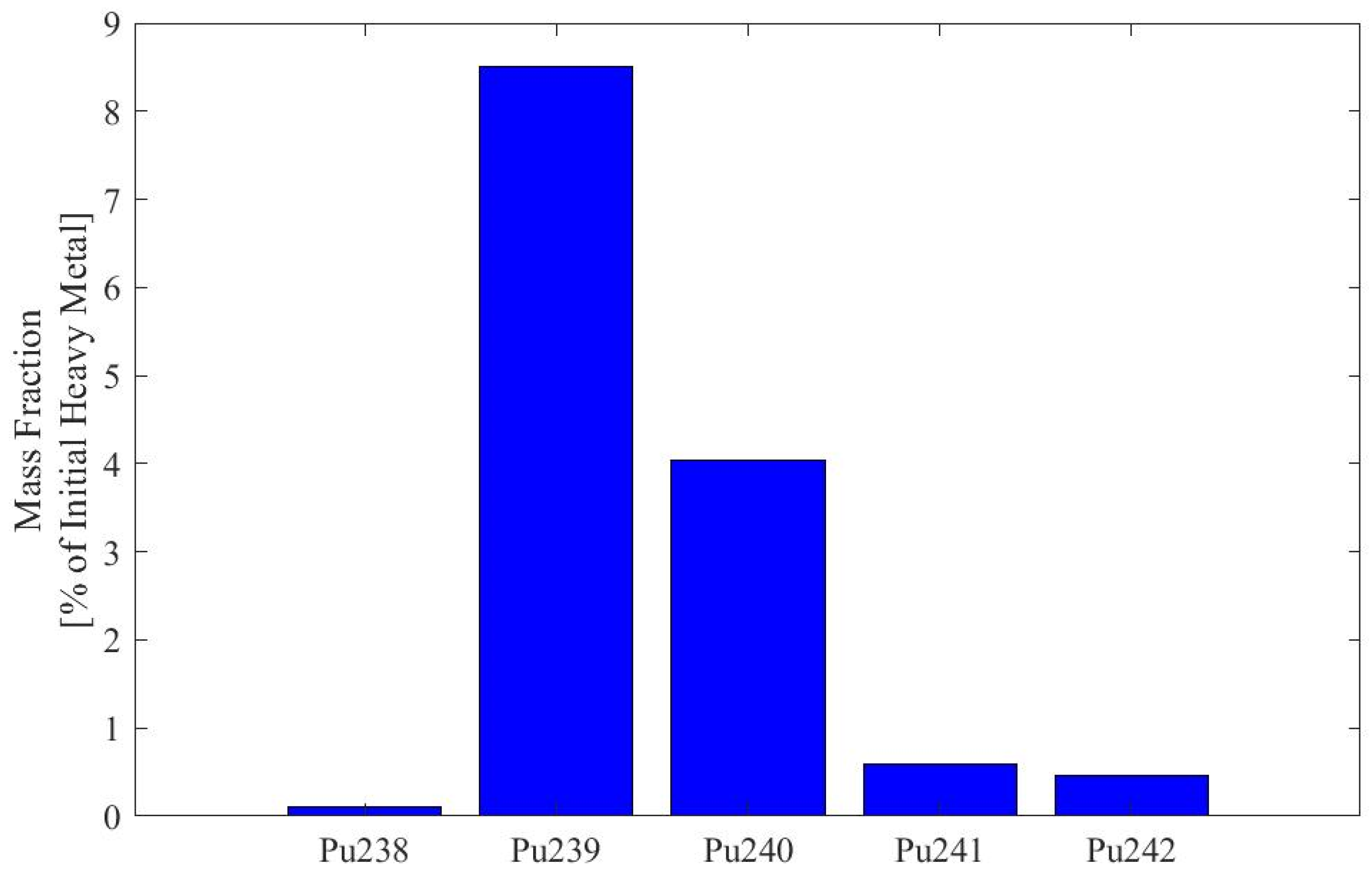
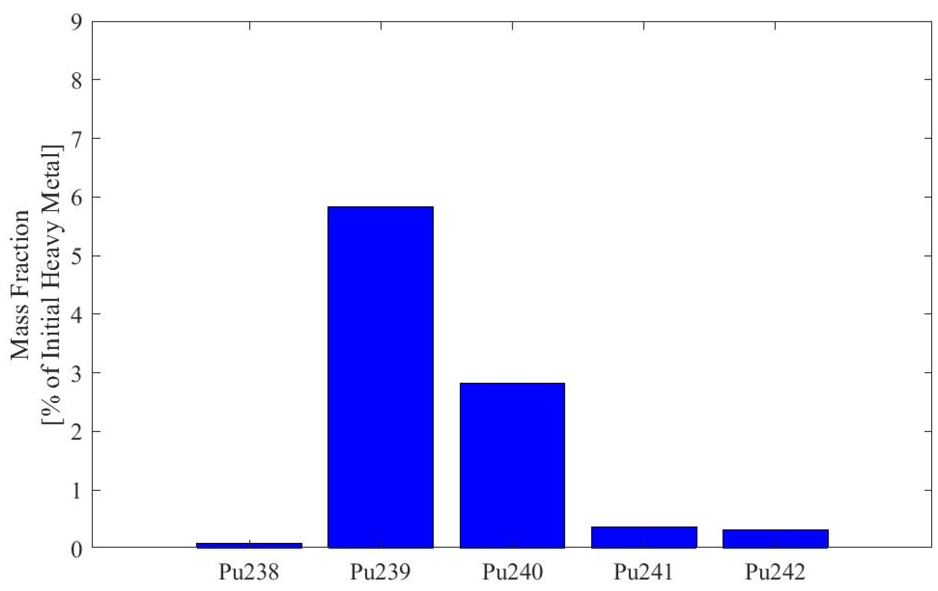
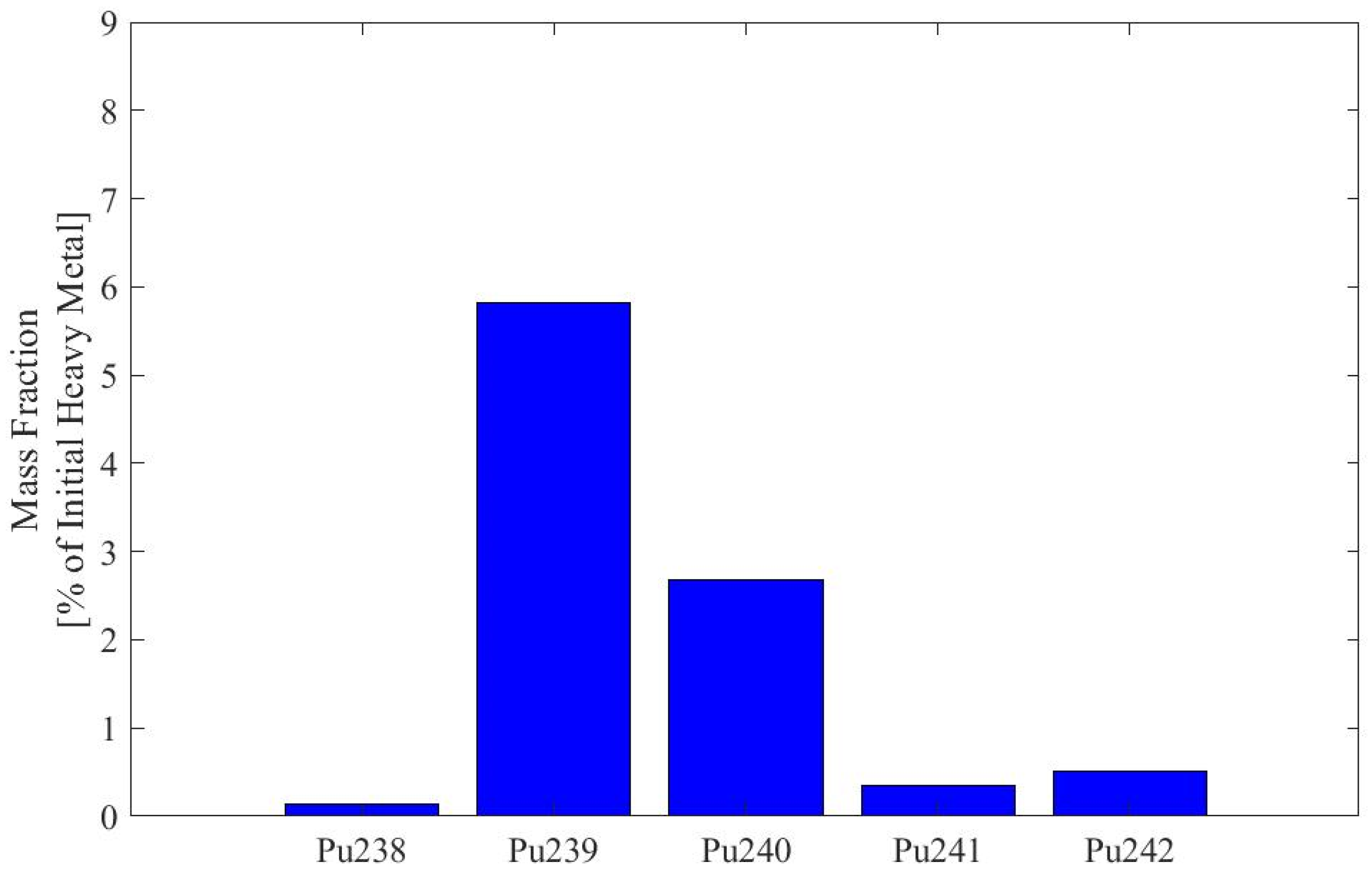
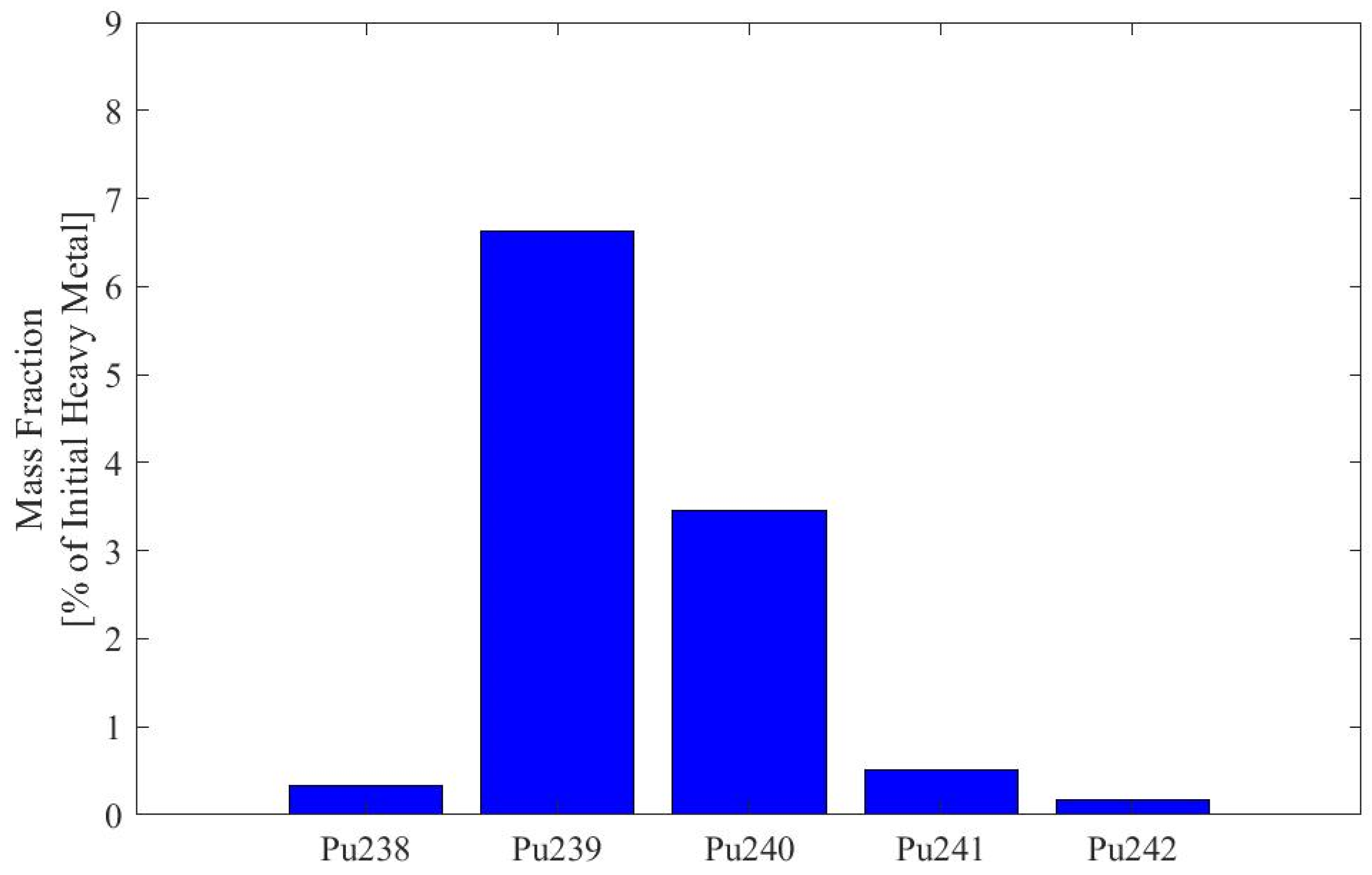
The plutonium isotopics of the fresh SFR fuels containing plutonium are shown in Table 3 for each relevant dataset. The plutonium isotopics of each fuel type that was depleted in SFR pincell simulations are shown in Figure A1, Figure A2, Figure A3, Figure A4, Figure A5, Figure A6, Figure A7 and Figure A8 in Appendix A.

2.2. Convolutional Neural Network

The CNN developed in this work was a residual network [14] similar to the models developed in [9,10]. Residual networks are characterized by the inclusion of skip connections between shallower and deeper layers that bypass layers in between. Residual networks are used to reduce the impact of vanishing gradients during training [15]. A simple, manually guided optimization was conducted where the activation function and number of filters in each convolutional layer of the CNN in [10] were varied. It was found that using ELU activations in place of rectified linear units (ReLUs) and increasing the number of filters from 128 to 256 improved the validation loss. The CNN was developed using the TensorFlow [16] library’s Keras API and was trained for 2500 epochs using the Adam optimization algorithm. Training proceeded with a batch size of 100 and an initial learning rate of 10−4. The learning rate was reduced to 2 × 10⁻⁵, 1 × 10⁻⁵, and 2 × 10⁻⁶ after 4000, 8000, and 16,000 training steps, respectively. The mean absolute error (MAE) loss metric was used as a basis for updating the weights and biases of the network during training. The validation dataset was used to compute a validation MAE loss score independent of the training loss. The weights and biases of the CNN that achieved the lowest validation loss score over 2500 epochs were stored and used to generate results in this work.
Because procedurally generated assemblies varied in size, the grids on which the mesh tallies were recorded also varied in their number of horizontal and vertical elements. To allow training to be conducted in a batch mode using stochastic gradient descent, each training sample’s input low-resolution tallies were segmented into equal-size non-overlapping 20 × 20 × 8 grids. The ground-truth high-resolution tallies were segmented into corresponding 40 × 40 × 16 grids. The training and inference pipeline included the data pre- and post-processing steps that scaled the input low-resolution data and output high-resolution prediction. All tally values in each sample were first multiplied by the total number of elements in that sample’s mesh. Again, this was done because generated assemblies varied in size, causing the recorded flux per mesh element in larger assemblies to be reduced compared with smaller assemblies. In a second scaling step, the largest flux value was sought for each energy group across the entire set of training data. These flux values were found in both the low- and high-resolution tallies in the training dataset. The input low-resolution tallies and output upsampled tallies were then divided by the largest flux values on a groupwise basis. The largest flux values in the training data were stored for use during inference on unseen validation and test data, where the high-resolution tallies are unknown to the CNN.

3. Results and Discussion

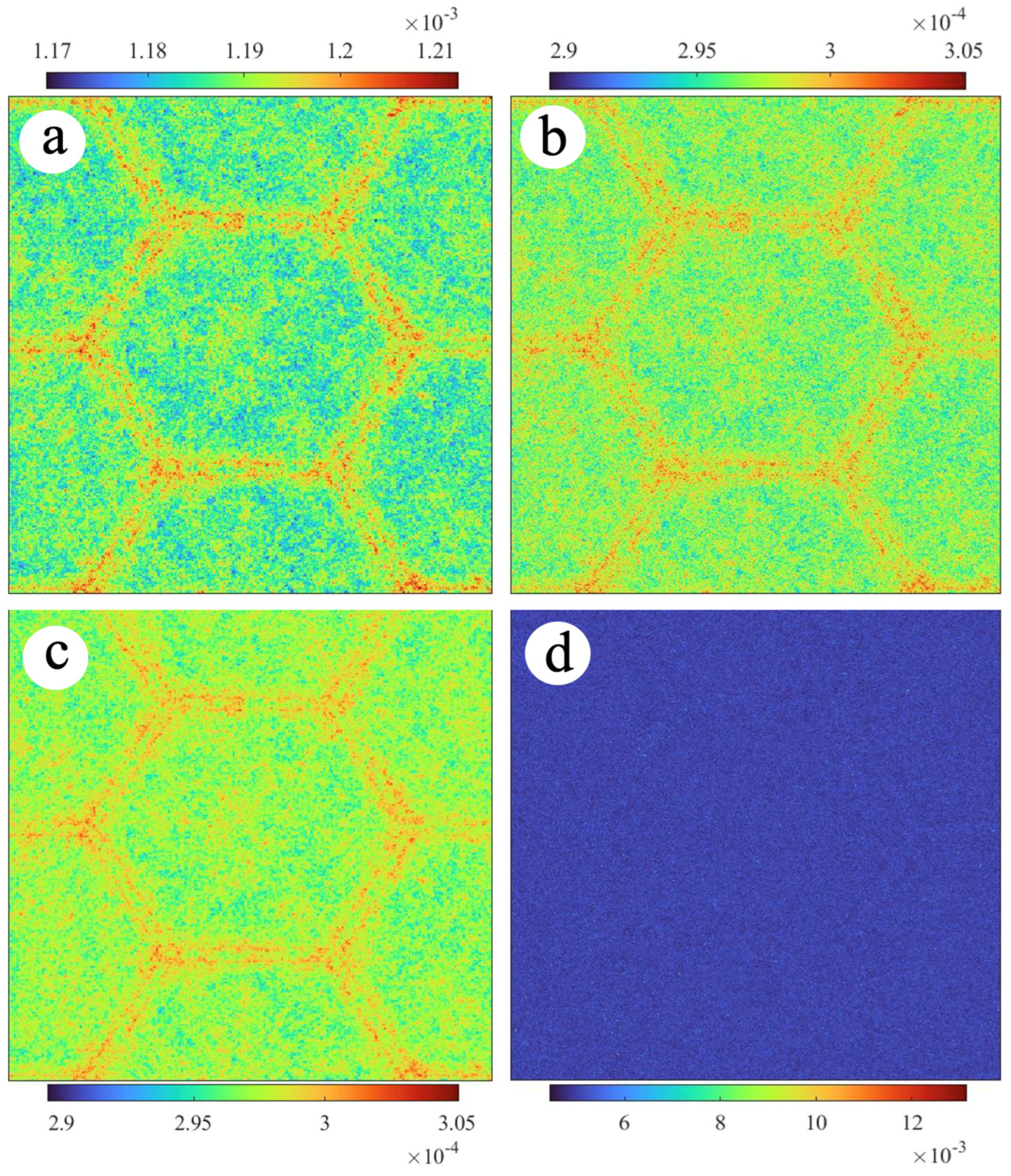
Figure 6 shows the low- and high-resolution neutron flux mesh tallies and relative error from the simulation corresponding to dataset K, as well as the upsampled CNN prediction. Dataset K (Table 2) corresponds to the simulation of the ESFR assembly. In this figure, the mesh tally fluxes are summed in the energy dimension. The relative error was calculated by summing absolute errors in quadrature along the energy dimension and dividing them by the flux. The upsampling prediction in Figure 6c compares well visually with the high-resolution OpenMC tally in Figure 6b. Figure 6d shows that the relative Monte Carlo uncertainty computed by OpenMC is close to 0.5% across the entire assembly.
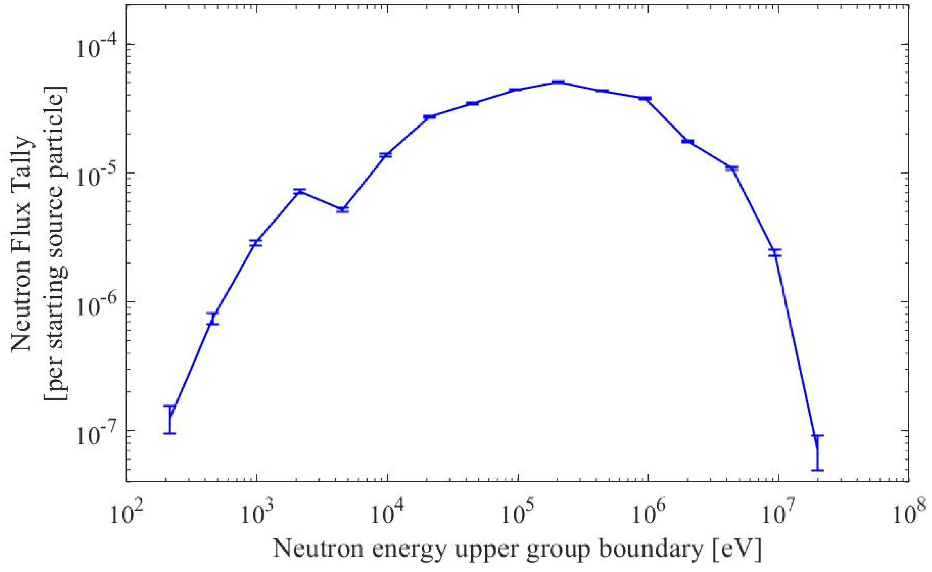
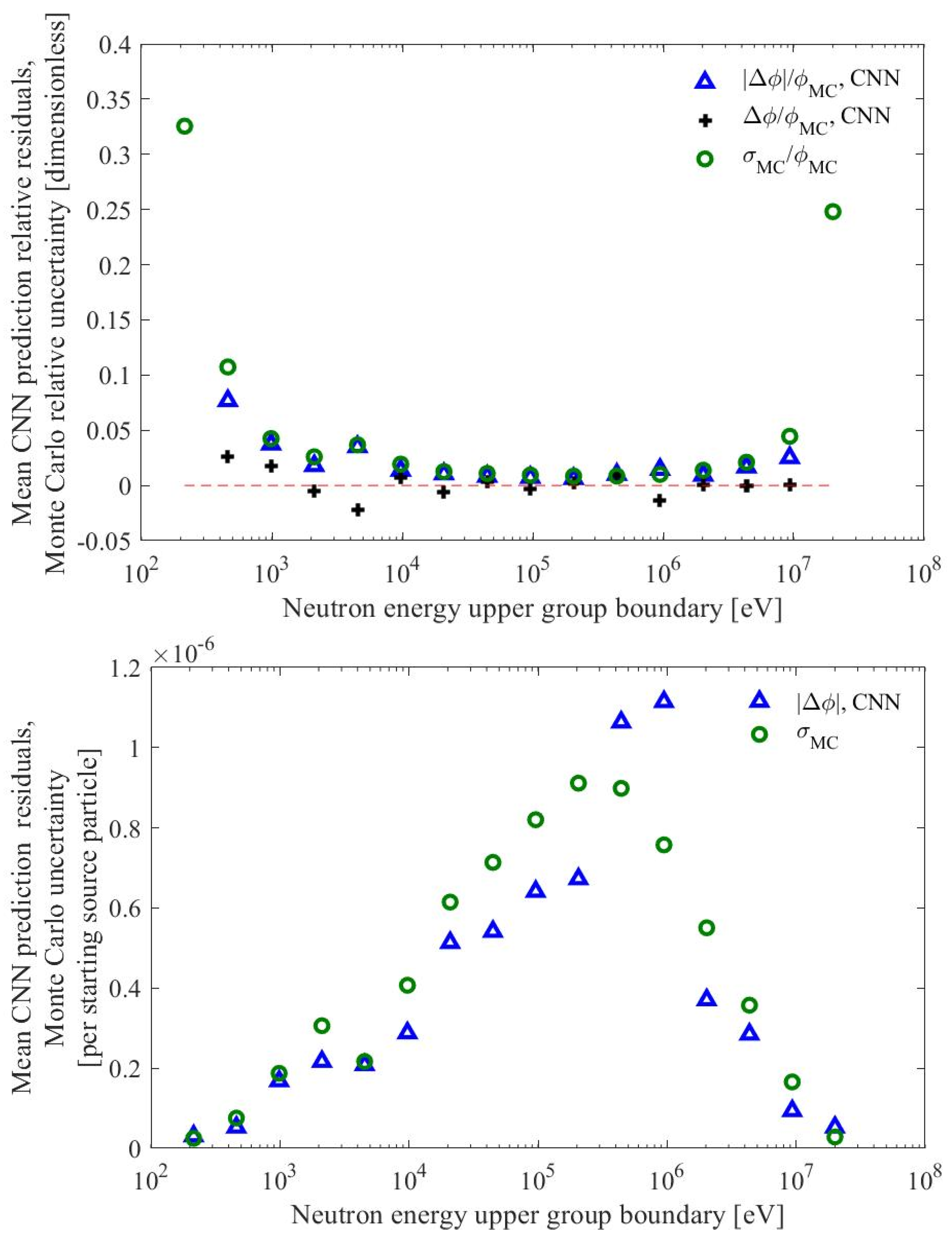
Figure 7 compares the residuals between the high-resolution OpenMC tally and the upsampled CNN prediction for dataset K as a function of neutron energy on relative and absolute bases. The mean residuals and errors are shown for each energy group, which is averaged across all spatial locations. The results in Figure 7 show that CNN’s prediction residual significantly exceeds the relative error computed using OpenMC only in the first and last energy groups. In all other energy groups, the CNN’s predictions were either within or very close to the Monte Carlo errors on a relative basis. This was the case for all energy groups when results were computed on an absolute basis. The figure also shows that CNN’s predictions only had a strong bias in the first and last energy groups. The neutron flux in these groups, however, was extremely low relative to that of other groups. Monte Carlo uncertainties scaled with the square root of the number of samples, which amplified the relative uncertainty in the energy groups with low statistics. The average neutron flux for dataset K is shown in the Appendix A, Figure A9.
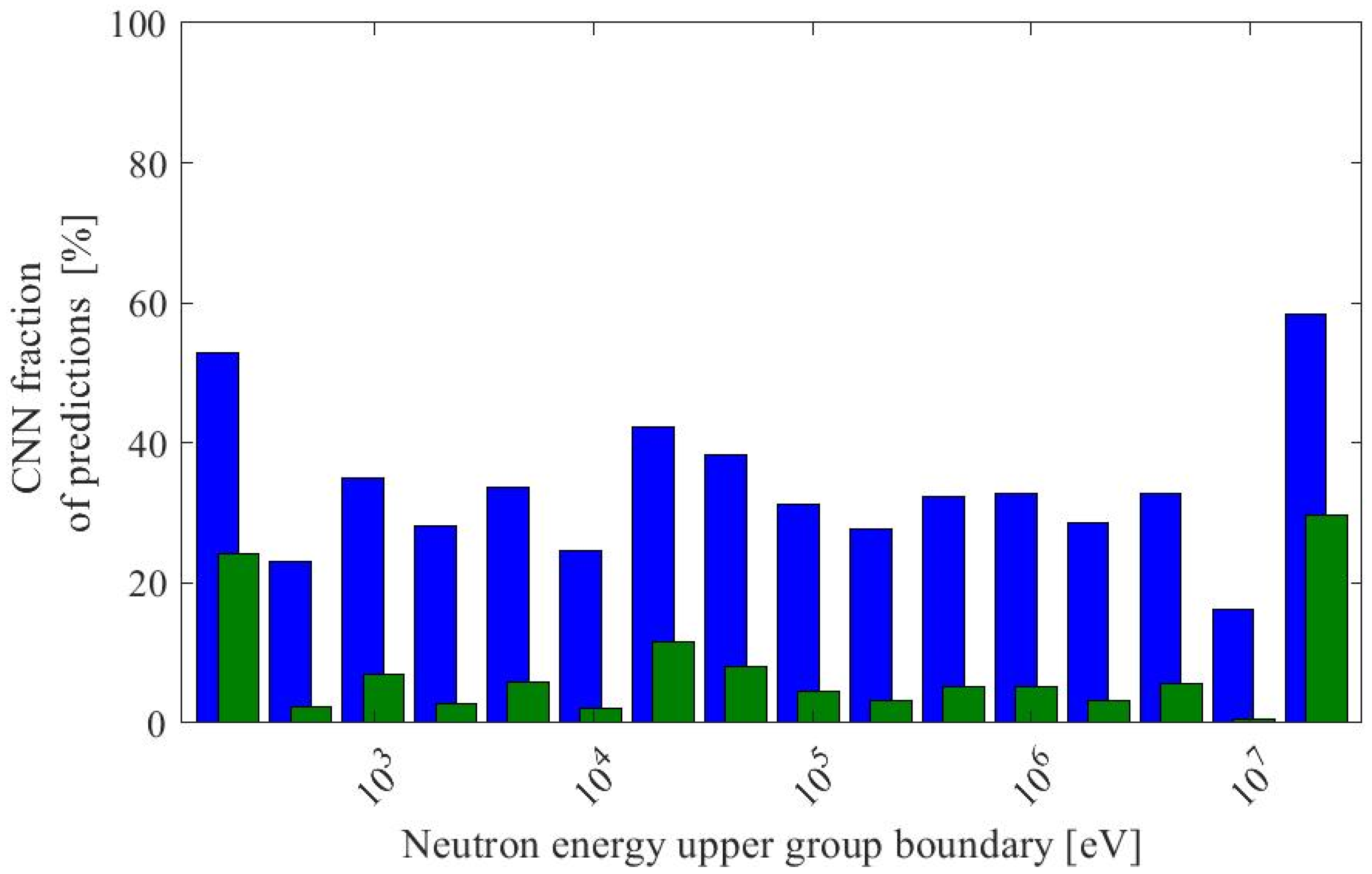
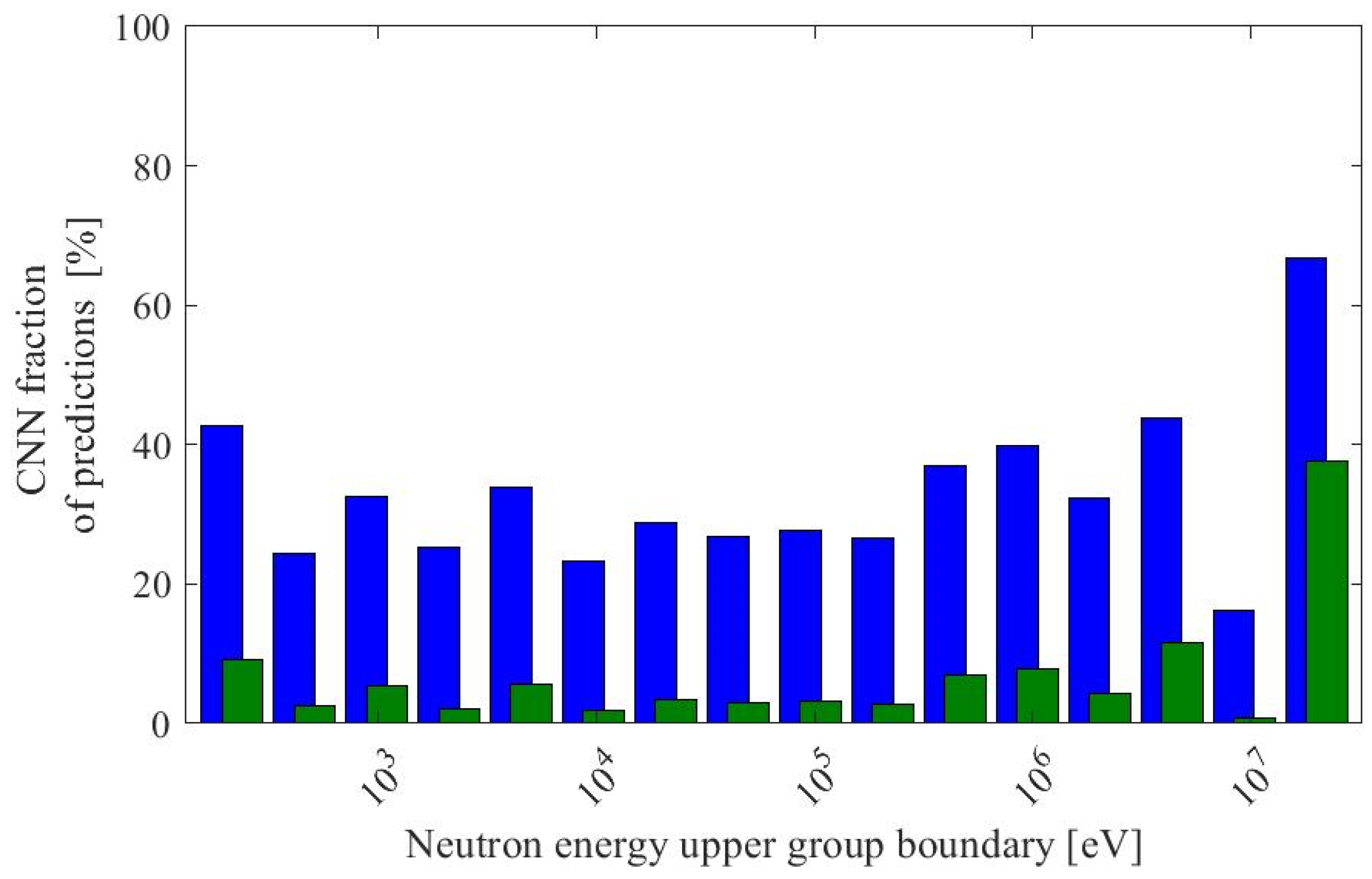
The number of CNN predictions worse than the Monte Carlo uncertainties is a useful metric for additional insight into its prediction accuracy. Figure 8 shows the fraction of CNN predictions outside one and two standard deviations of the Monte Carlo calculation for dataset K. CNN’s predictions were outside one and two standard deviations in 33.6% and 7.6% of cases overall, respectively. These numbers align closely with what would be expected, assuming that errors are normally distributed. By using this metric, the prediction accuracy was reduced at very low and high energies where the flux was low. The results shown in Figure 7 and Figure 8 are tabulated in the Appendix, Table A1.
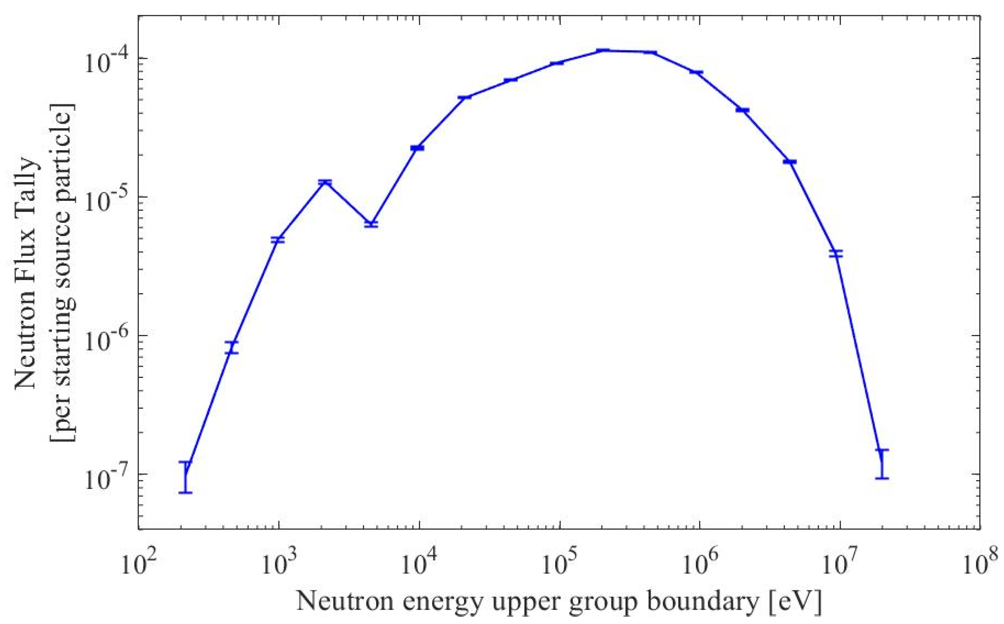
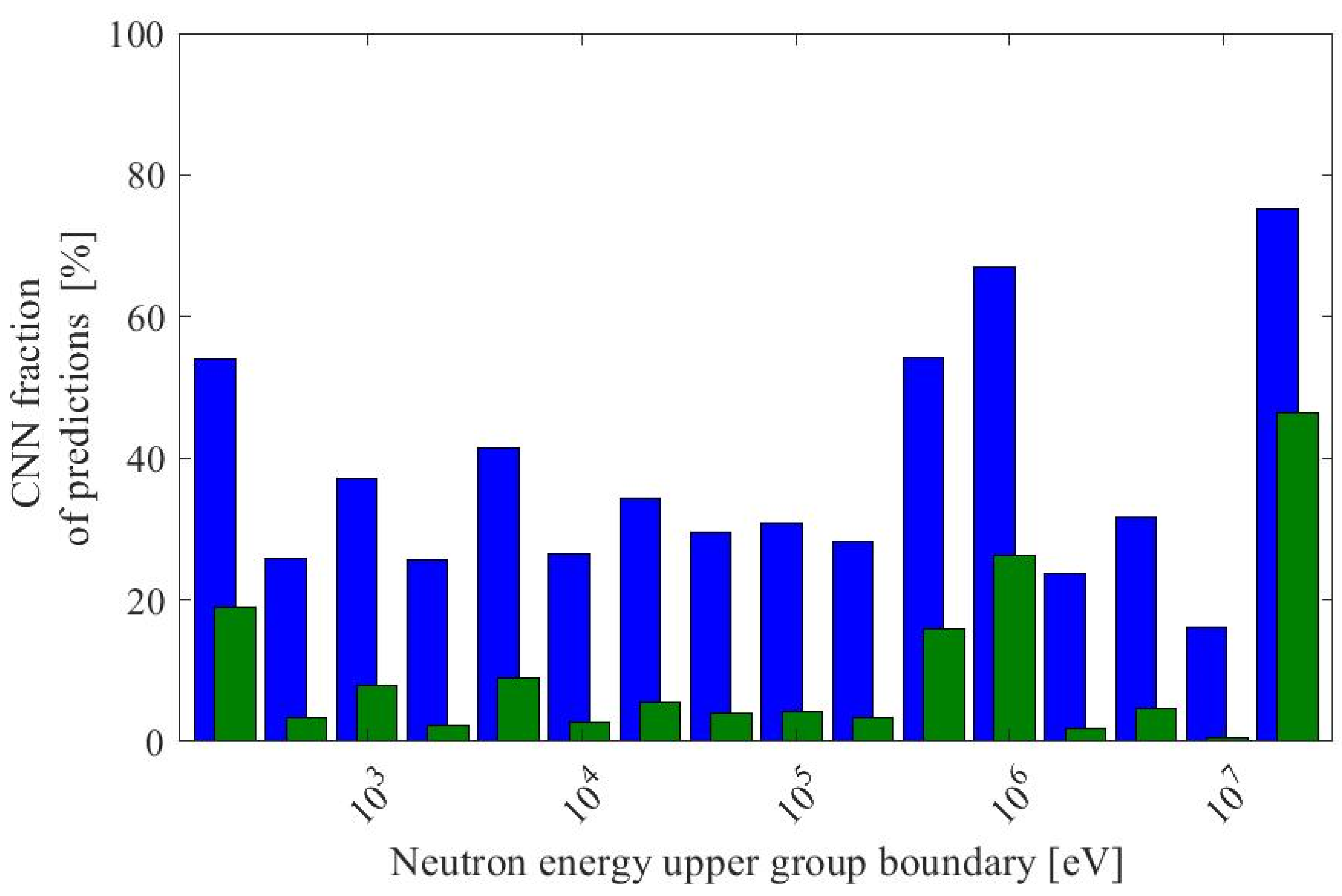
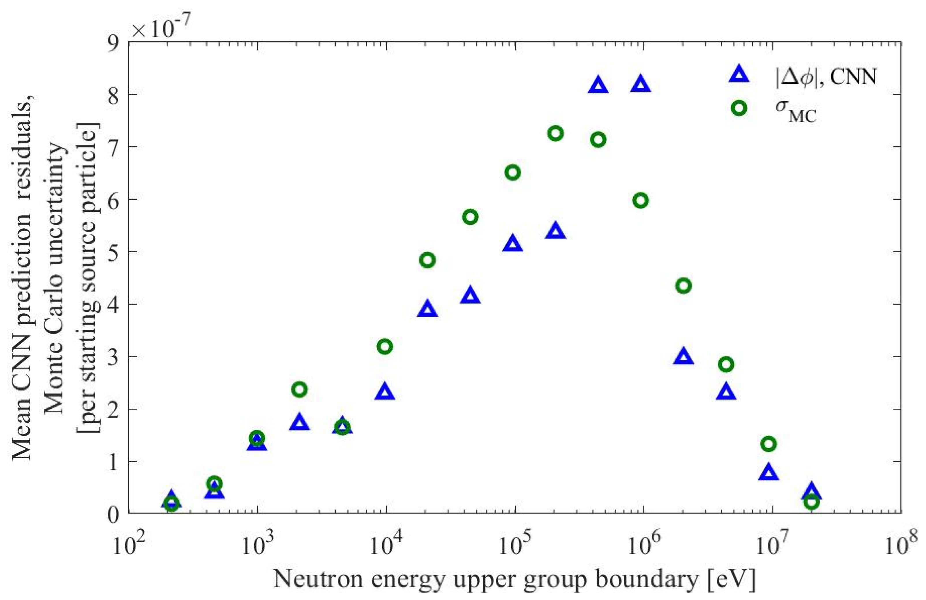
The CNN prediction residuals and Monte Carlo uncertainties are compared for the test dataset L in Figure 9. This dataset comprised procedurally generated assemblies with 10 or 11 rings of pins whose fuel’s plutonium isotopes were taken from discharged LWR fuel enriched to 1.6%. In the assemblies of dataset L, the fuel form was UPuZr with burnup values between 220 and 400 MWd/kgIHM, burned in a fast spectrum. Figure 10 shows the fraction of CNN predictions outside one and two Monte Carlo standard deviations for dataset L. On a relative basis, the mean residuals in the CNN’s predictions were close to or below the Monte Carlo uncertainty, except for the low and high energy groups. Again, these energies correspond to very low neutron fluxes. The prediction bias in either direction was also small except in the groups with low neutron flux values. Unlike dataset K, in dataset L, the mean values of the CNN’s residuals were larger than Monte Carlo uncertainties around 200 to 950 keV. On a relative basis, however, the residuals in this region were 1.45% at worst. The average neutron flux for dataset L is shown in the Appendix A, Figure A10.
Figure 10 shows the fraction of CNN predictions outside one and two Monte Carlo standard deviations for dataset L. CNN’s predictions were outside one and two standard deviations in 37.6% and 9.8% of cases overall, respectively. The results shown in Figure 9 and Figure 10 are tabulated in the Appendix A, Table A2.
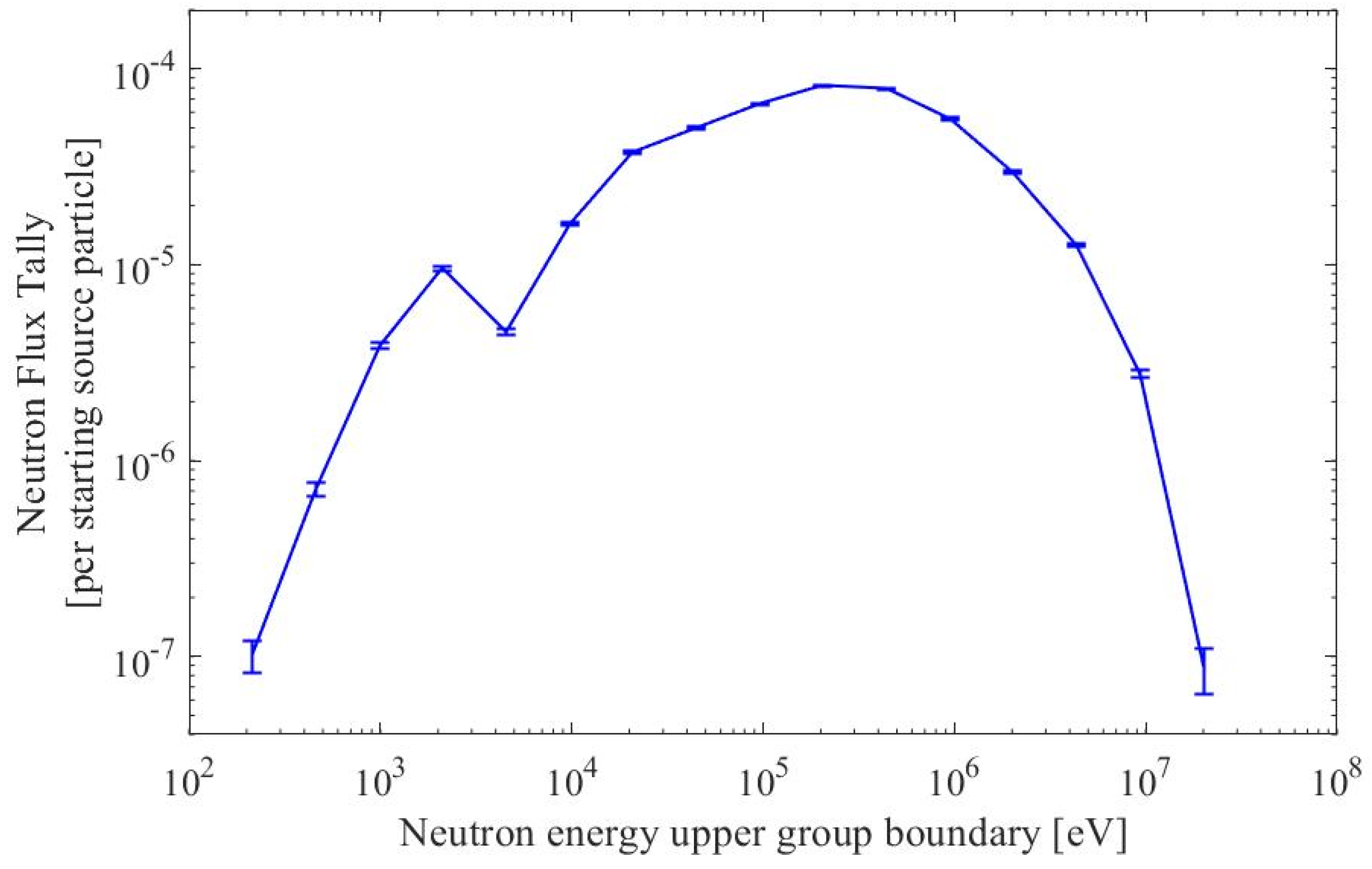
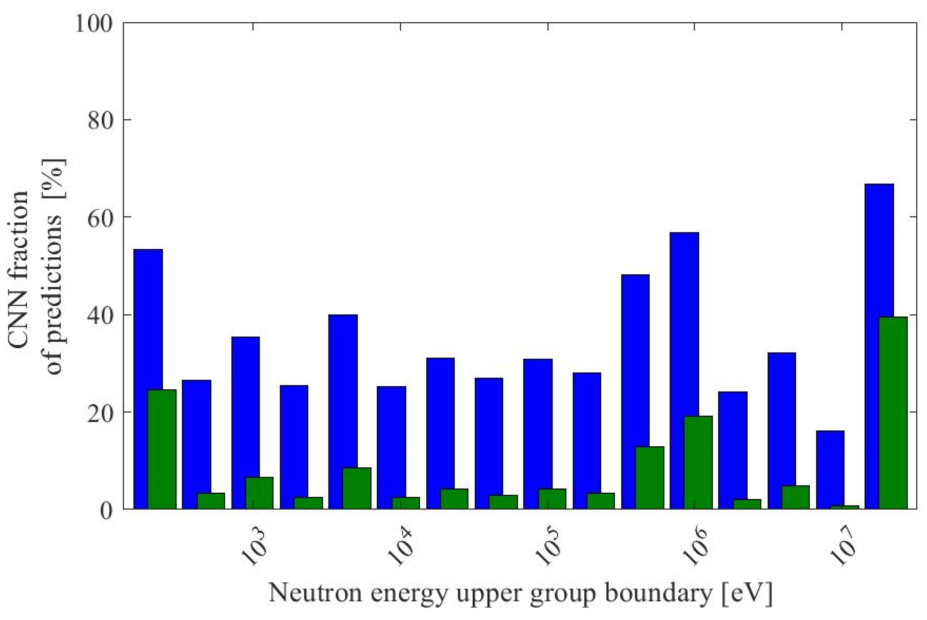
Figure 11 shows a comparison between the CNN prediction residuals and Monte Carlo uncertainties for test dataset M. This dataset comprised procedurally generated assemblies with 10 or 11 rings of pins whose fuel’s plutonium isotopes were taken from discharged LWR fuel enriched to 19.9%. In the assemblies of dataset M, the fuel form was UPuZr with burnup values between 220 and 400 MWd/kgIHM, burned in a fast spectrum. The accuracy of the CNN’s predictions, as well as the prediction bias, on dataset M varied by energy in a similar manner to dataset L. Although the absolute residuals between 200 and 950 keV were larger than Monte Carlo uncertainty, on a relative basis, this corresponded to 1.64% at worst. The average neutron flux for dataset M is shown in the Appendix A, Figure A11.
Figure 12 shows the fraction of CNN predictions outside one and two Monte Carlo standard deviations for dataset M. CNN’s predictions were outside one and two standard deviations in 35.4% and 8.9% of cases overall, respectively. The results shown in Figure 11 and Figure 12 are tabulated in the Appendix A, Table A3.
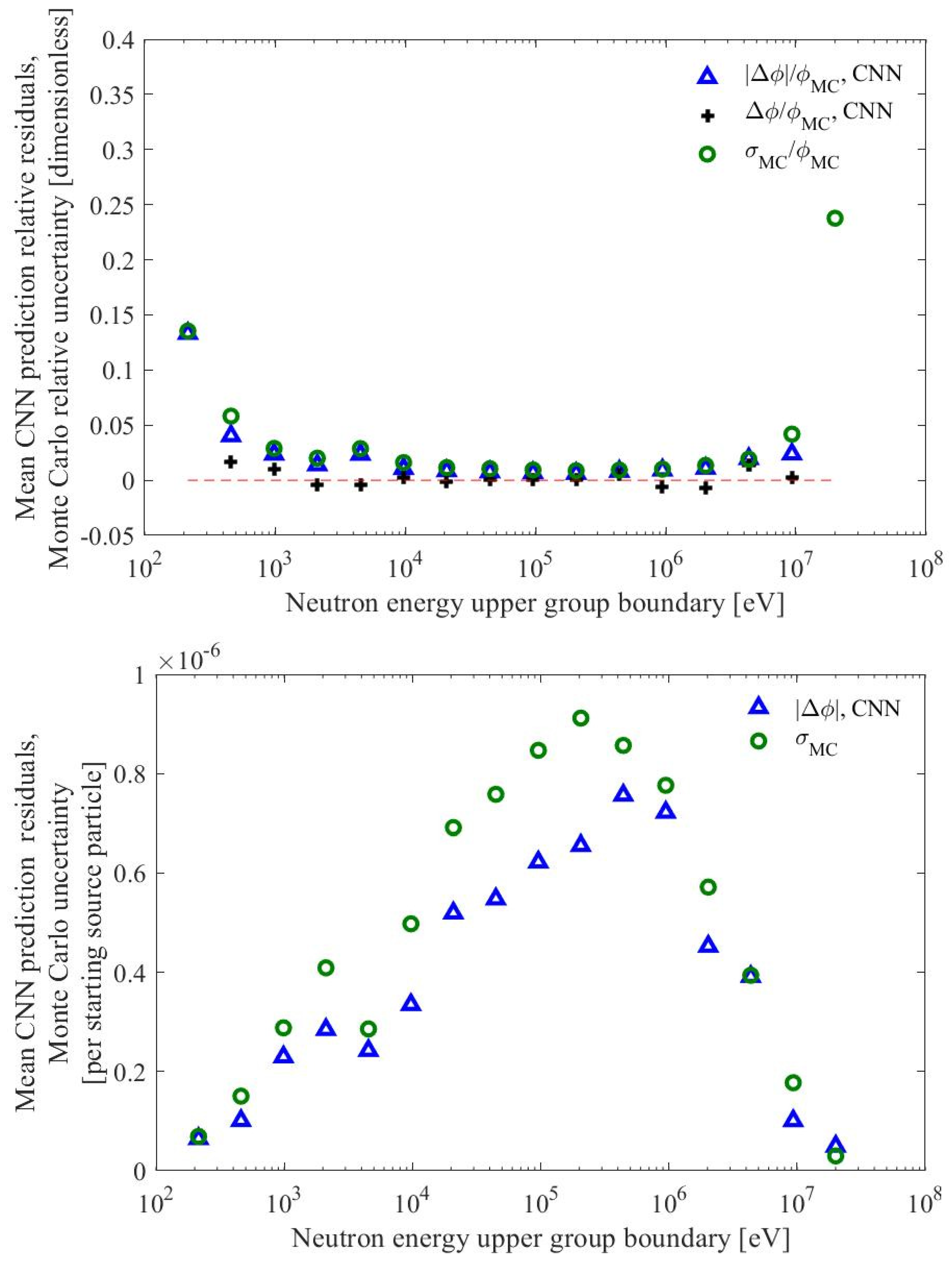
The CNN prediction accuracy for datasets N and O was extremely close to or below the Monte Carlo uncertainties in almost all energy groups, as shown in Figure 13. The sole exception to this was at the highest energy group and only on a relative basis. Because of this, Figure 13 represents the combined statistics of datasets N and O. Prediction biases were also small and, overall, did not show a preference in direction, except for the lowest and highest energy groups. Similarly, Figure 14 shows the fraction of CNN predictions outside one and two Monte Carlo standard deviations for datasets N and O, again using combined statistics for both datasets. CNN’s predictions were outside one and two standard deviations in 33.0% and 6.8% of cases overall, respectively. The results shown in Figure 13 and Figure 14 are tabulated in the Appendix A, Table A4. The average neutron flux for datasets N and O is shown in the Appendix A, Figure A12.
The predictions made by the CNN on unseen test data were accurate on a relative basis, except in energy groups where the neutron flux was close to zero, as shown in Figure 7, Figure 9, Figure 11, and Figure 13. This was also the case on an absolute basis, with the only exceptions being in the 200–950 keV region in high burnup procedurally generated test assemblies fueled with UPuZr, as shown in Figure 9, Figure 10, Figure 11 and Figure 12. Even in these cases, the difference between the CNN predictions’ residuals, 1.64%, and the Monte Carlo uncertainty, 1.37%, was extremely small compared with the neutron flux. In the MOX or UOX test assemblies burned up to 400 MWd/kgIHM, however, the CNN residuals remained smaller than the Monte Carlo uncertainties in the 200–950 keV region, as shown in Figure 7 and Figure 13. A likely explanation for this difference is that the fissile plutonium content in UPuZr fuel is lower than that in the MOX or UOX fuel at high levels of burnup. Even in the high-burnup MOX and UOX samples (Datasets N, O, Figure 13), the predictive accuracy of the CNN in the 200–950 keV region was slightly worse compared with the ESFR assembly predictions, as shown in Figure 7. In the ESFR assembly, the plutonium content of the fuel was high, which is closer in similarity to the training data in contrast to the high-burnup datasets. Prediction biases generally do not show a strong directional preference except for energy groups with very low flux values.
An important feature of the CNN trained in this work is the relatively small number of assemblies in its training dataset. CNNs in previous studies were trained using 4400 [9] and 5568 [10] unique assemblies, while the CNN in this work was trained with 300 assemblies. Despite this, the CNN achieved similar accuracy as measured by the fraction of predictions below one and two Monte Carlo standard deviations, as shown in Figure 8, Figure 10, Figure 12, and Figure 14. The neutron flux tallies in this work, however, were recorded on a mesh with spatial elements less than a third of the width of the meshes in [9,10]. By pixel count, the training data in this work would be comparable.

4. Conclusions and Future Work

A residual convolutional neural network was trained on neutron flux tally data computed using OpenMC. The training data consisted of 250 samples of low- and high-resolution flux tallies from fast reactor simulations and 50 samples from thermal spectrum simulations. All training data samples consisted of hexagonal assemblies with two to five rings of pins, with fuel burnup up to 180 MWd/kgIHM. Validation data consisted of eight samples of fast reactor assemblies with 10 or 11 rings of pins and fuel burnup up to 180 MWd/kgIHM. All samples in the training and validation data were heterogeneous procedurally generated assemblies using Latin hypercube sampling to select assembly- and pin-level geometric and material parameters. To test the CNN, eight procedurally generated heterogeneous fast reactor assemblies were simulated with burnup levels from 220 to 400 MWd/kgIHM and 10 or 11 rings of pins. The burnup range was selected to test CNN’s ability to generalize in samples with characteristics that were well outside those encountered in the training data. The CNN was also tested on a simulation of a realistic ESFR assembly with fresh mixed-oxide fuel.
The results show that across all test and validation data, the fraction of predictions outside one (two) standard deviation was 36% (8.6%) and 31% (6.8%), respectively. The residuals and fraction of predictions outside one and two standard deviations were also given by the energy group for individual test datasets. In all test data and energy groups, the residuals were smaller than or close to the Monte Carlo uncertainty on an absolute basis. On a relative basis, this is also the case, with the exception being at energies above 20 MeV, where the neutron flux was close to zero.
Although the CNN trained in this work can make accurate predictions on test data that are considerably dissimilar to the training data, it is limited to specific resolutions. The CNN can upsample 1 × 1 mm tallies to 0.5 × 0.5 mm accurately, but a CNN that can operate on a wider range of input and output resolutions would be of significant utility. Similarly, a CNN with the ability to upsample between different input and output energy resolutions would also be valuable. Similar neural network models, such as generative adversarial networks (GANs), could be explored to enable this capability. GANs have been shown previously to be effective in the super-resolution of climatological data [17], and similar benefits of GANs could be realized in the context of neutron transport simulations. Incorporating uncertainty quantification methods to enable the neural network to estimate the confidence in upsampled predictions would also be essential before its use in neutron Monte Carlo applications. Ensemble methods have been shown to provide uncertainty quantification in simulations of neutron flux monitors [18] and could be adapted for upsampling in a similar way. Finally, the potential for the flexible and accurate upsampling of neutron flux tallies using additional input data that would be available a priori has not been explored. Another CNN input layer could accept a spatial map of the materials used as input to the Monte Carlo simulation. This input layer would be connected to the existing input and encode valuable additional information that would be propagated to downstream layers. Alternatively, or in addition, other types of prior information, such as uncertainties and few-group cross-sections, could be encoded in CNN input layers.

Author Contributions

Conceptualization, A.O.; Methodology, A.O.; Software, J.B. and A.O.; Validation, P.R. and A.O.; Formal analysis, J.B.; Investigation, J.B.; Resources, P.R. and A.O.; Writing—original draft, A.O.; Writing—review & editing, J.B. and P.R.; Supervision, A.O.; Project administration, A.O.; Funding acquisition, A.O. All authors have read and agreed to the published version of the manuscript.

Funding

This research was supported by the Exascale Computing Project (17-SC-20-SC), a collaborative effort of the U.S. Department of Energy Office of Science and the National Nuclear Security Administration. and the APC was funded by The Colorado School of Mines.

Data Availability Statement

Software and data related to this work are available at zenodo.org under DOI: https://zenodo.org/doi/10.5281/zenodo.10703159 [13].

Acknowledgments

We gratefully acknowledge the computing resources provided on Bebop, a high-performance computing cluster operated by the Laboratory Computing Resource Center at Argonne National Laboratory. The submitted manuscript has been created by UChicago Argonne, LLC, Operator of Argonne National Laboratory (“Argonne”). Argonne, a U.S. Department of Energy Office of Science laboratory, is operated under Contract No. DE-AC02-06CH11357. The U.S. Government retains for itself, and others acting on its behalf, a paid-up nonexclusive, irrevocable worldwide license in said article to reproduce, prepare derivative works, distribute copies to the public, and perform publicly and display publicly, by or on behalf of the Government. The Department of Energy will provide public access to these results of federally sponsored research in accordance with the DOE Public Access Plan. http://energy.gov/downloads/doe-public-access-plan, accessed on 26 February 2024.

Conflicts of Interest

The authors declare no conflicts of interest.

Appendix A. Plutonium Isotopics of Fuel Depleted in SFR Pincell Simulations
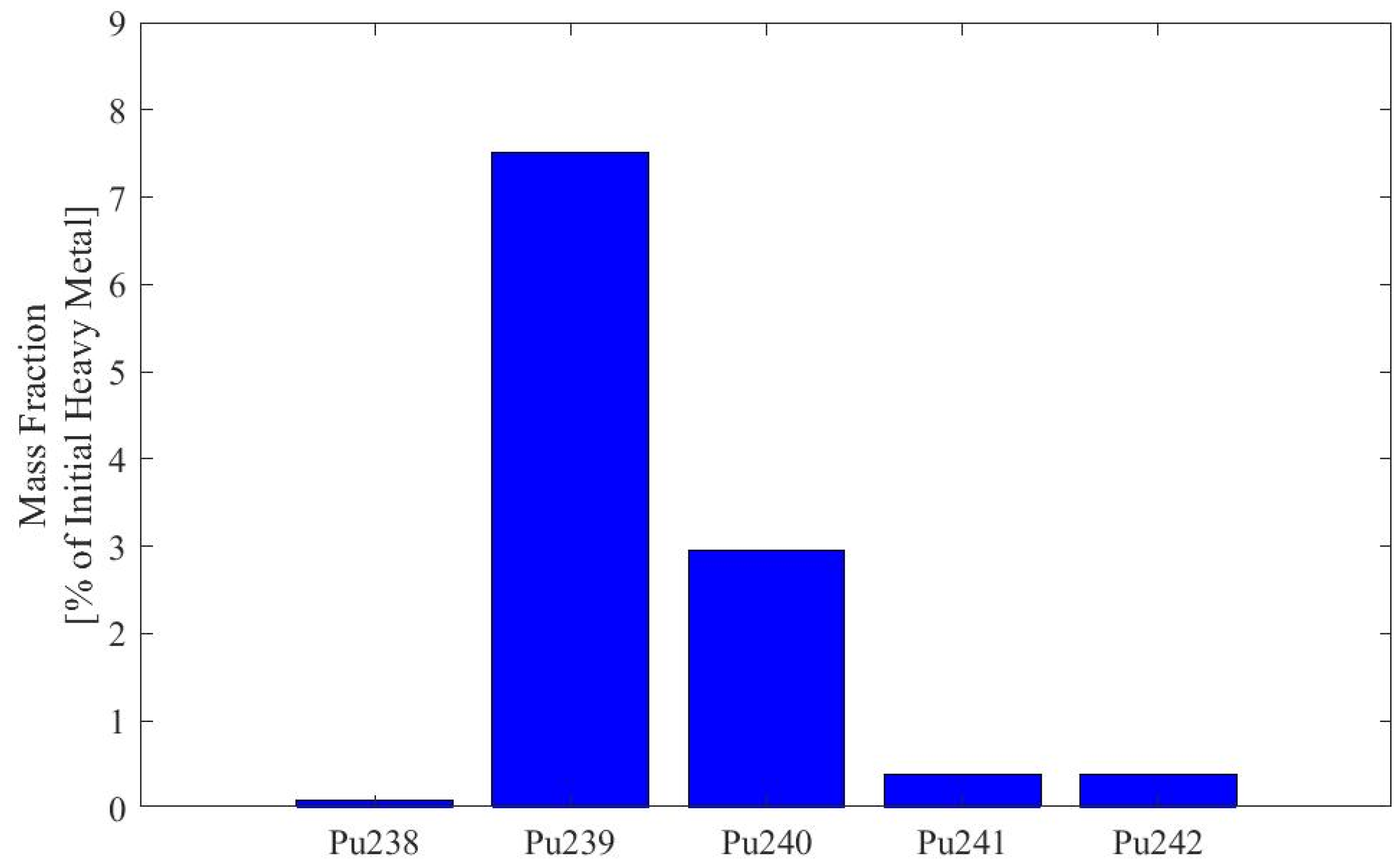
Figure A1. Plutonium isotopics, UPuZr fuel. The Pu in the UPuZr fuel burned in the SFR pincell simulation originated from 1.6% enriched UOX burned in an LWR simulation to 17.44 MWd/kgIHM. The isotopics shown correspond to UPuZr fuel at 180 MWd/kgIHM of burnup in an SFR spectrum. Relevant datasets using this type of fuel are A and G (Figure 3 and Figure 4).
Energies 17 02177 g0a1
Figure A2. Plutonium Isotopics, UPuZr fuel. The Pu in the UPuZr fuel burned in the SFR pincell simulation originated from 19.9% enriched UOX burned in an LWR simulation to 216.91 MWd/kgIHM. The isotopics shown correspond to UPuZr fuel at 180 MWd/kgIHM of burnup in an SFR spectrum. Dataset H includes this type of fuel (Figure 4).
Energies 17 02177 g0a2
Figure A3. Plutonium Isotopics, UOX fuel. The isotopics shown correspond to 11% enriched UOX fuel at 180 MWd/kgIHM of burnup in an SFR spectrum. Relevant datasets using this type of fuel are B and I (Figure 3 and Figure 4).
Energies 17 02177 g0a3
Figure A4. Plutonium Isotopics, MOX fuel. The Pu in the MOX fuel burned in the SFR pincell simulation originated from 1.6% enriched UOX burned in an LWR simulation to 17.44 MWd/kgIHM. The isotopics shown correspond to MOX fuel at 180 MWd/kgIHM of burnup in an SFR spectrum. Dataset J includes this type of fuel (Figure 4).
Energies 17 02177 g0a4
Figure A5. Plutonium Isotopics, UPuZr fuel. The Pu in the UPuZr fuel burned in the SFR pincell simulation originated from 1.6% enriched UOX burned in an LWR simulation to 17.44 MWd/kgIHM. The isotopics shown correspond to MOX fuel at 400 MWd/kgIHM of burnup in an SFR spectrum. Dataset L includes this type of fuel (Figure 5).
Energies 17 02177 g0a5
Figure A6. Plutonium Isotopics, UPuZr fuel. The Pu in the UPuZr fuel burned in the SFR pincell simulation originated from 19.9% enriched UOX burned in an LWR simulation to 216.91 MWd/kgIHM. The isotopics shown correspond to MOX fuel at 400 MWd/kgIHM of burnup in an SFR spectrum. Dataset M includes this type of fuel (Figure 5).
Energies 17 02177 g0a6
Figure A7. Plutonium Isotopics, UOX fuel. The isotopics shown correspond to 11% enriched UOX fuel at 400 MWd/kgIHM of burnup in an SFR spectrum. Dataset N includes this type of fuel (Figure 5).
Energies 17 02177 g0a7
Figure A8. Plutonium Isotopics, MOX fuel. The Pu in the MOX fuel burned in the SFR pincell simulation originated from 1.6% enriched UOX burned in an LWR simulation to 17.44 MWd/kgIHM. The isotopics shown correspond to MOX fuel at 400 MWd/kgIHM of burnup in an SFR spectrum. Dataset O includes this type of fuel (Figure 5).
Energies 17 02177 g0a8
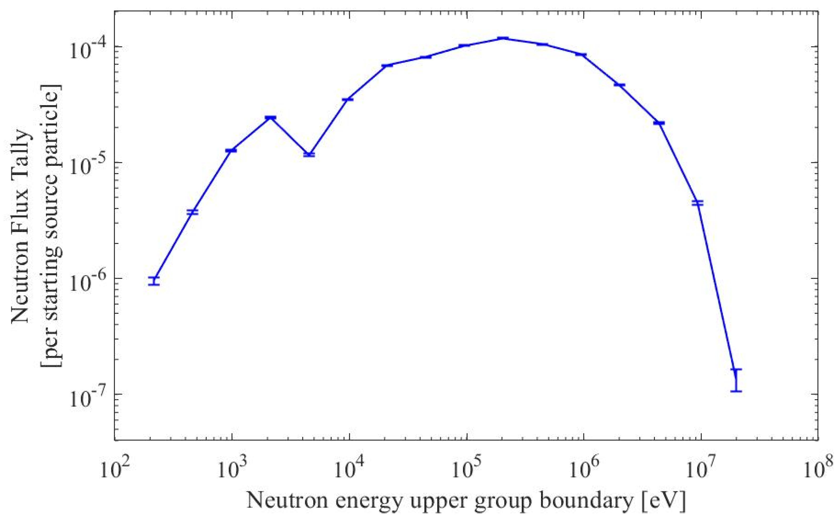
  • Neutron Flux Plots: Test Datasets
Figure A9. Neutron flux tally in dataset K. Each data point represents an average over each spatial element of the assembly in dataset K. Error bars represent the average Monte Carlo uncertainty also across each spatial element in dataset K.
Energies 17 02177 g0a9
Figure A10. Neutron flux tally in dataset L. Each data point represents an average over each spatial element in both samples in dataset L. Error bars represent the average Monte Carlo uncertainty also over each spatial element in dataset L.
Energies 17 02177 g0a10
Figure A11. Neutron flux tally in dataset M. Each data point represents an average over all spatial tally bins of both samples in dataset M. Error bars represent the average Monte Carlo uncertainty also across all spatial tally bins in dataset M.
Energies 17 02177 g0a11
Figure A12. Neutron flux tally in datasets N and O. Each data point represents an average over all spatial tally bins of all four samples in datasets N and O. Error bars represent the average Monte Carlo uncertainty also over all spatial tally bins in datasets N and O.
Energies 17 02177 g0a12
  • Tabulated Data: Test Datasets
Table A1. Tabulated data for Figure 7 and Figure 8, dataset K. Lowest error for each group is in bold.
Upper Energy Bin [eV]MC Relative Error [%]CNN Relative Residual [%]CNN Relative Residual Bias [%]MC Absolute Error aCNN Absolute Residual aFraction of Predictions Worse Than MC Uncertainty [%]
1σ2σ
2.14 × 10224.3834.8529.562.98 × 10−83.64 × 10−852.8824.25
4.60 × 10210.066.761.157.43 × 10−84.91 × 10−823.142.27
9.86 × 1025.144.442.101.47 × 10−71.24 × 10−735.057.02
2.11 × 1033.262.39−1.242.34 × 10−71.72 × 10−728.072.67
4.53 × 1033.863.220.871.99 × 10−71.65 × 10−733.725.94
9.72 × 1032.371.62−0.453.23 × 10−72.22 × 10−724.532.01
2.09 × 1041.671.681.214.52 × 10−74.49 × 10−742.2711.65
4.47 × 1041.491.35−0.915.12 × 10−74.70 × 10−738.218.11
9.59 × 1041.311.040.435.77 × 10−74.53 × 10−731.164.59
2.06 × 1051.220.900.146.17 × 10−74.50 × 10−727.643.17
4.41 × 1051.321.070.205.70 × 10−74.60 × 10−732.395.18
9.46 × 1051.401.14−0.045.32 × 10−74.32 × 10−732.845.08
2.03 × 1062.061.53−0.653.59 × 10−72.68 × 10−728.483.10
4.35 × 1062.612.130.852.82 × 10−72.28 × 10−732.685.56
9.33 × 1065.523.14−0.051.32 × 10−77.47 × 10−816.200.64
2.00 × 10731.5753.9050.442.16 × 10−82.83 × 10−858.4129.68
a Units are per starting source particle.
Table A2. Tabulated data for Figure 9 and Figure 10, dataset L. Lowest error for each group in bold.
Upper Energy Bin [eV]MC Relative Error [%]CNN Relative Residual [%]CNN Relative Residual Bias [%]MC Absolute Error aCNN Absolute Residual aFraction of Predictions Worse Than MC Uncertainty [%]
1σ2σ
2.14 × 10232.5543.74−8.212.48 × 10−83.08 × 10−854.0718.94
4.60 × 10210.737.682.657.54 × 10−85.27 × 10−825.883.39
9.86 × 1024.253.741.781.87 × 10−71.68 × 10−737.057.95
2.11 × 1032.591.79−0.493.06 × 10−72.17 × 10−725.552.23
4.53 × 1033.683.51−2.222.17 × 10−72.08 × 10−741.358.98
9.72 × 1031.931.370.744.07 × 10−72.88 × 10−726.482.78
2.09 × 1041.261.05−0.566.15 × 10−75.14 × 10−734.305.45
4.47 × 1041.080.830.367.14 × 10−75.41 × 10−729.623.90
9.59 × 1040.940.73−0.318.21 × 10−76.42 × 10−730.864.13
2.06 × 1050.840.620.229.12 × 10−76.73 × 10−728.223.35
4.41 × 1050.851.000.908.99 × 10−71.06 × 10−654.1515.94
9.46 × 1051.011.45−1.397.58 × 10−71.11 × 10−667.0026.27
2.03 × 1061.380.930.025.51 × 10−73.71 × 10−723.741.93
4.35 × 1062.101.67−0.033.57 × 10−72.85 × 10−731.724.75
9.33 × 1064.452.520.071.66 × 10−79.37 × 10−816.060.64
2.00 × 10724.8153.1152.092.84 × 10−85.25 × 10−875.2146.35
a Units are per starting source particle.
Table A3. Tabulated data for Figure 11 and Figure 12, dataset M. Lowest error for each group in bold.
Upper Energy Bin [eV]MC Relative Error [%]CNN Relative Residual [%]CNN Relative Residual Bias [%]MC Absolute Error aCNN Absolute Residual aFraction of Predictions Worse Than MC Uncertainty [%]
1σ2σ
2.14 × 10259.16282.61196.201.91 × 10−82.41 × 10−853.4524.56
4.60 × 10217.9513.111.375.68 × 10−84.04 × 10−826.423.37
9.86 × 1026.485.37−0.071.44 × 10−71.32 × 10−735.396.49
2.11 × 1033.812.620.472.37 × 10−71.72 × 10−725.422.55
4.53 × 1035.434.89−2.061.65 × 10−71.65 × 10−739.978.49
9.72 × 1032.711.850.733.19 × 10−72.30 × 10−725.272.57
2.09 × 1041.761.36−0.504.84 × 10−73.88 × 10−731.004.16
4.47 × 1041.491.060.275.67 × 10−74.14 × 10−726.872.99
9.59 × 1041.281.00−0.366.52 × 10−75.12 × 10−730.854.12
2.06 × 1051.140.850.277.26 × 10−75.37 × 10−728.123.36
4.41 × 1051.161.201.007.14 × 10−78.15 × 10−748.1012.96
9.46 × 1051.371.64−1.465.98 × 10−78.17 × 10−756.8919.07
2.03 × 1061.871.27−0.014.35 × 10−72.97 × 10−724.242.05
4.35 × 1062.802.240.162.85 × 10−72.30 × 10−732.084.92
9.33 × 1065.863.330.091.33 × 10−77.54 × 10−816.130.68
2.00 × 10732.8866.8764.302.27 × 10−83.94 × 10−866.7139.41
a Units are per starting source particle.
Table A4. Tabulated data for Figs. 13,14, datasets N and O. Lowest error for each group in bold.
Upper Energy Bin [eV]MC Relative Error [%]CNN Relative Residual [%]CNN Relative Residual Bias [%]MC Absolute Error aCNN Absolute Residual aFraction of Predictions Worse Than MC Uncertainty [%]
1σ2σ
2.14 × 10213.5313.32−7.236.92 × 10−86.47 × 10−842.669.18
4.60 × 1025.824.031.661.50 × 10−71.01 × 10−724.442.63
9.86 × 1022.892.361.012.88 × 10−72.30 × 10−732.455.41
2.11 × 1032.011.39−0.444.09 × 10−72.85 × 10−725.242.19
4.53 × 1032.872.35−0.422.86 × 10−72.42 × 10−733.875.55
9.72 × 1031.611.060.254.98 × 10−73.35 × 10−723.261.91
2.09 × 1041.150.86−0.106.91 × 10−75.19 × 10−728.843.49
4.47 × 1041.050.750.057.58 × 10−75.48 × 10−726.922.90
9.59 × 1040.930.680.028.47 × 10−76.22 × 10−727.773.16
2.06 × 1050.860.620.059.12 × 10−76.55 × 10−726.702.83
4.41 × 1050.920.810.548.57 × 10−77.56 × 10−737.077.01
9.46 × 1051.000.93−0.657.76 × 10−77.22 × 10−739.797.94
2.03 × 1061.351.08−0.665.72 × 10−74.52 × 10−732.244.24
4.35 × 1061.921.961.393.94 × 10−73.91 × 10−743.7811.59
9.33 × 1064.192.380.211.77 × 10−71.01 × 10−716.260.70
2.00 × 10723.7743.0341.122.99 × 10−84.94 × 10−866.7837.54
a Units are per starting source particle.

References

  1. Leppänen, J.; Pusa, M.; Viitanen, T.; Valtavirta, V.; Kaltiaisenaho, T. The Serpent Monte Carlo code: Status, development and applications in 2013. Ann. Nucl. Energy 2015, 82, 142–150. [Google Scholar] [CrossRef]
  2. Romano, P.K.; Horelik, N.E.; Herman, B.R.; Nelson, A.G.; Forget, B.; Smith, K. OpenMC: A state-of-the-art Monte Carlo code for research and development. Ann. Nucl. Energy 2015, 82, 90–97. [Google Scholar] [CrossRef]
  3. Werner, C.J.; Brown, F.B.; Bull, J.S.; Casswell, L.; Cox, L.J.; Dixon, D.; Forster, R.A. MCNP® User’s Manual, Code Version 6.2; Los Alamos National Laboratory: Los Alamos, NM, USA, 2017. [Google Scholar]
  4. Wendt, B.; Kerby, L.; Tumulak, A.; Leppänen, J. Advancement of functional expansion capabilities: Implementation and optimization in Serpent 2. Nucl. Eng. Des. 2018, 334, 138–153. [Google Scholar] [CrossRef]
  5. Horelik, N.; Siegel, A.; Forget, B.; Smith, K. Monte Carlo domain decomposition for robust nuclear reactor analysis. Parallel Comput. 2014, 40, 646–660. [Google Scholar] [CrossRef]
  6. García, M.; Leppänen, J.; Sanchez-Espinoza, V. A Collision-based Domain Decomposition scheme for large-scale depletion with the Serpent 2 Monte Carlo code. Ann. Nucl. Energy 2021, 152, 108026. [Google Scholar] [CrossRef]
  7. Vaquer, P.A.; McClarren, R.G.; Ayzman, Y.J. A Compressed Sensing Framework for Monte Carlo Transport Simulations Using Random Disjoint Tallies. J. Comput. Theor. Transp. 2016, 45, 219–229. [Google Scholar] [CrossRef]
  8. Madsen, J.R. Disjoint Tally Method: A Monte Carlo Scoring Method Using Compressed Sensing to Reduce Statistical Noise and Memory. Ph.D. Thesis, Texas A&M University, College Station, TX, USA, 2017. [Google Scholar]
  9. Osborne, A.; Dorville, J.; Romano, P. Upsampling Monte Carlo neutron transport simulation tallies using a convolutional neural network. Energy AI 2023, 13, 100247. [Google Scholar] [CrossRef]
  10. Berry, J.; Romano, P.; Osborne, A. Upsampling Monte Carlo reactor simulation tallies in depleted LWR assemblies fueled with LEU and HALEU using a convolutional neural network. AIP Adv. 2024, 14, 015004. [Google Scholar] [CrossRef]
  11. Facchini, A.; Giusti, V.; Ciolini, R.; Tuček, K.; Thomas, D.; D’Agata, E. Detailed neutronic study of the power evolution for the European Sodium Fast Reactor during a positive insertion of reactivity. Nucl. Eng. Des. 2017, 313, 1–9. [Google Scholar] [CrossRef]
  12. Brown, D.A.; Chadwick, M.B.; Capote, R.; Kahler, A.C.; Trkov, A.; Herman, M.W.; Sonzogni, A.A.; Danon, Y.; Carlson, A.D.; Dunn, M.; et al. ENDF/B-VIII.0: The 8th Major Release of the Nuclear Reaction Data Library with CIELO-project Cross Sections, New Standards and Thermal Scattering Data. Nuclear Data Sheets 2018, 148, 1–142. [Google Scholar] [CrossRef]
  13. Berry, J.; Romano, P.; Osborne, A. Data and Software: Upsampling Monte Carlo Reactor Simulation Tallies in Depleted SFR Assemblies using a Convolutional Neural Network 2024. AIP Adv. 2024, 14, 015004. [Google Scholar] [CrossRef]
  14. Lim, B.; Son, S.; Kim, H.; Nah, S.; Lee, K.M. Enhanced Deep Residual Networks for Single Image Super-Resolution. In Proceedings of the 2017 IEEE Conference on Computer Vision and Pattern Recognition Workshops (CVPRW), Honolulu, HI, USA, 21–26 July 2017; IEEE: Piscataway, NJ, USA, 2017; pp. 1132–1140. [Google Scholar]
  15. He, K.; Zhang, X.; Ren, S.; Sun, J. Deep Residual Learning for Image Recognition. In Proceedings of the 2016 IEEE Conference on Computer Vision and Pattern Recognition (CVPR), Las Vegas, NV, USA, 27–30 June 2016; IEEE: Piscataway, NJ, USA, 2016; pp. 770–778. [Google Scholar]
  16. Abadi, M.; Agarwal, A.; Barham, P.; Brevdo, E.; Chen, Z.; Citro, C.; Corrado, G.S.; Davis, A.; Dean, J.; Devin, M.; et al. TensorFlow: Large-Scale Machine Learning on Heterogeneous Systems. arXiv 2015, arXiv:1603.04467. [Google Scholar]
  17. Stengel, K.; Glaws, A.; Hettinger, D.; King, R.N. Adversarial super-resolution of climatological wind and solar data. Proc. Natl. Acad. Sci. USA 2020, 117, 16805–16815. [Google Scholar] [CrossRef]
  18. Wilkinson, I.M.; Bhattacharjee, R.R.; Shafer, J.C.; Osborne, A.G. Confidence estimation in the prediction of epithermal neutron resonance self-shielding factors in irradiation samples using an ensemble neural network. Energy AI 2022, 7, 100131. [Google Scholar] [CrossRef]
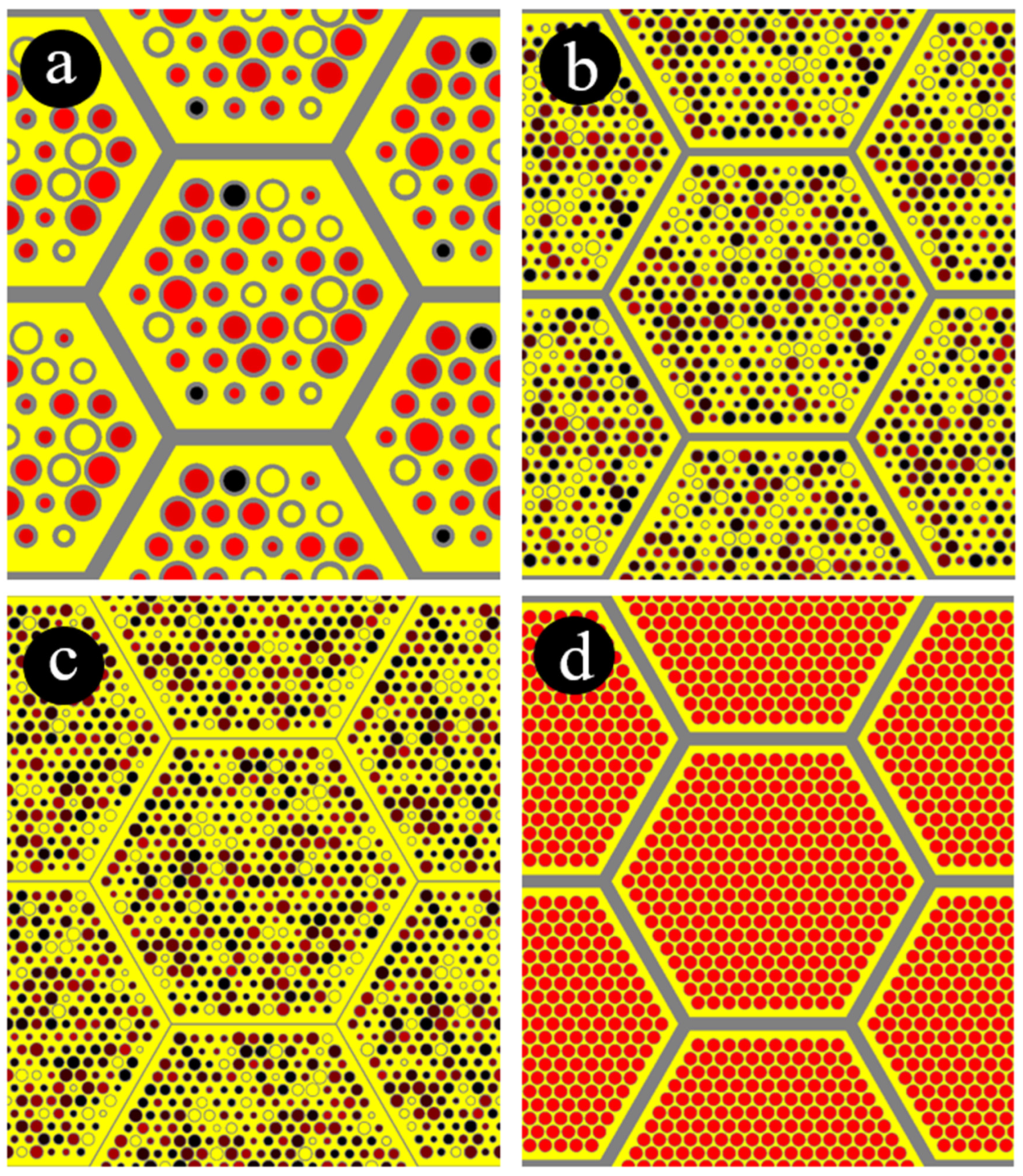
Figure 1. Representative sample assembly geometries. Assemblies are not shown to scale. (a) Assembly geometry in a sample from a training dataset. The assembly has 4 rings of pins containing fresh fuel (red pins), B4C (black pins), or sodium (yellow pins). (b) Assembly geometry in a sample from a validation dataset. The assembly has 10 rings of pins containing fuel with burnup values ranging from fresh (0 MWd/kgIHM) to 180 MWd/kgIHM. Darker shades of red represent fuel with higher burnup values. (c) Assembly geometry in a sample from a test dataset. The assembly has 11 rings of pins with burnup values ranging from 220 to 400 MWd/kgIHM. (d) Assembly geometry in the ESFR test assembly. All pins contain fresh fuel.
Energies 17 02177 g001
Figure 2. Pincell depletion simulation geometry. The fuel, cladding, and coolant are shown in red, gray, and yellow, respectively. Reflective boundary conditions are placed on the inner hexagonal duct surfaces.
Energies 17 02177 g002
Figure 3. Fuel origin flowchart for training datasets. Fuel in datasets A, E, and D originate from an LWR depletion simulation performed in [10]. The plutonium isotopics from the fuel burned to 17.44 MWd/kgIHM in an LWR spectrum are sampled and reformulated as UPuZr (A, E) and MOX (D) fuel. The UPuZr is then burned in an SFR simulation up to 180 MWd/kgIHM in steps of 20 MWd/kgIHM (A) before being used in criticality eigenvalue assembly-level simulations. Datasets D and E are imported directly into the assembly simulations as fresh MOX and UPuZr, respectively. Dataset B is UOX fuel enriched to 11%, burned in an SFR simulation, and used in the assembly simulations. Datasets C and F are fresh UOX and U imported directly into the assembly simulations without being burned. Dataset D contains assembly simulations with water coolant to increase the diversity of the neutron flux spectra in the training data. Quantities of U and Pu in UPuZr fuel are percentages of total heavy metal.
Energies 17 02177 g003
Figure 4. Fuel origin flowchart for validation datasets. Fuel in datasets G, J, and H originates from LWR depletion simulations of UOX fuel enriched to 1.6% (G, J) and 19.9% (H) performed in [10]. The plutonium isotopics from the fuel burned to 17.44 MWd/kgIHM (G, J) or 216.91 MWd/kgIHM (H) in an LWR spectrum are sampled and reformulated as UPuZr (G, H) and MOX (J) fuels. Fuel in dataset I begins as fresh UOX enriched to 11%. All fuel types in validation datasets are then burned in SFR pincell depletion simulations up to 180 MWd/kgIHM in steps of 20 MWd/kgIHM before being used in criticality eigenvalue assembly-level simulations. Quantities of U and Pu in UPuZr fuel are percentages of total heavy metal.
Energies 17 02177 g004
Figure 5. Fuel origin flowchart for test datasets. Fuel in datasets L, O, and M originates from LWR depletion simulations of UOX fuel enriched to 1.6% (L, O) and 19.9% (M) performed in [10]. The plutonium isotopics from the fuel burned to 17.44 MWd/kgIHM (L, O) or 216.91 MWd/kgIHM (M) in an LWR spectrum are sampled and reformulated as UPuZr (L, M) and MOX (O) fuels. Fuel in dataset N begins as fresh UOX enriched to 11%. All fuel types in test datasets M, N, L, and O are then burned in SFR pincell depletion simulations from 220 to 400 MWd/kgIHM in steps of 20 MWd/kgIHM before being used in criticality eigenvalue assembly-level simulations. Fuel in test dataset K originates from an ESFR reactor with isotopics, according to [11], and is imported directly into an assembly-level simulation. Quantities of U and Pu in UPuZr fuel are percentages of total heavy metal.
Energies 17 02177 g005
Figure 6. Neutron flux tallies, CNN prediction, and Monte Carlo relative error for ESFR assembly (dataset K). (a) Low-resolution neutron flux mesh tally computed using OpenMC. (b) High-resolution neutron flux mesh tally computed using OpenMC (ground truth). (c) Upsampled neutron flux tally predicted using CNN was a low-resolution tally (a) as input. (d) Relative error in the high-resolution tally (b) was computed using OpenMC. Units on colorbars of panels (ac) are in counts per starting source particle.
Energies 17 02177 g006
Figure 7. Mean CNN prediction residuals and Monte Carlo errors for ESFR assembly (dataset K). (Top) Blue triangles show the relative magnitude of the prediction residuals with respect to the Monte Carlo high-resolution flux tallies. Black crosses represent the relative residuals computed without the magnitude, which is shown to illustrate the prediction bias for each group. (Bottom) Absolute residuals and Monte Carlo errors. Each data point represents an average over each spatial element of the sample.
Energies 17 02177 g007
Figure 8. Fraction (%) of CNN predictions outside one (blue) and two (green) Monte Carlo standard deviations. Data points were computed by counting the number of CNN predictions with residuals greater than one and two Monte Carlo standard deviations and dividing them by the total number of data points.
Energies 17 02177 g008
Figure 9. Mean CNN prediction residuals and Monte Carlo errors for UPuZr assemblies (dataset L). (Top) Blue triangles show the relative magnitude of the prediction residuals with respect to the Monte Carlo high-resolution flux tallies. Black crosses represent the relative residuals computed without the magnitude, which is shown to illustrate the prediction bias for each group. (Bottom) Absolute residuals and Monte Carlo errors. Each data point represents an average over each spatial element of both samples in dataset L.
Energies 17 02177 g009
Figure 10. Fraction (%) of CNN predictions outside one (blue) and two (green) Monte Carlo standard deviations for UPuZr assemblies (dataset L). Data points were computed by counting the number of CNN predictions with residuals greater than one and two Monte Carlo standard deviations and dividing them by the total number of data points.
Energies 17 02177 g010
Figure 11. Mean CNN prediction residuals and Monte Carlo errors for UPuZr assemblies (dataset M). (Top) Blue triangles show the relative magnitude of the prediction residuals with respect to the Monte Carlo high-resolution flux tallies. Black crosses represent the relative residuals computed without the magnitude, which is shown to illustrate the prediction bias for each group. (Bottom) Absolute residuals and Monte Carlo errors. Each data point represents an average over each spatial element of both samples in dataset M.
Energies 17 02177 g011aEnergies 17 02177 g011b
Figure 12. Fraction (%) of CNN predictions outside one (blue) and two (green) Monte Carlo standard deviations for UPuZr assemblies (dataset M). Data points were computed by counting the number of CNN predictions with residuals greater than one and two Monte Carlo standard deviations and dividing them by the total number of data points.
Energies 17 02177 g012
Figure 13. Mean CNN prediction residuals and Monte Carlo errors for UOX and MOX test assemblies (datasets N, O). (Top) Blue triangles show the relative magnitude of the prediction residuals with respect to the Monte Carlo high-resolution flux tallies. Black crosses represent the relative residuals computed without the magnitude, which is shown to illustrate the prediction bias for each group. (Bottom) Absolute residuals and Monte Carlo errors. Each data point represents an average over each spatial element of a total of 4 samples across the two datasets.
Energies 17 02177 g013
Figure 14. Fraction (%) of CNN predictions outside one (blue) and two (green) Monte Carlo standard deviations for UOX and MOX test assemblies (datasets N, O). Data points were computed by counting the number of CNN predictions with residuals greater than one and two Monte Carlo standard deviations and dividing them by the total number of data points.
Energies 17 02177 g014
Table 1. Ranges of geometric parameters in assembly simulations.
ParameterRange (Procedurally
Generated Assemblies)
Value (ESFR
Test Assembly)
Pin Diameter a0.5 to 1.00.4715 cm
Pin Pitch [cm]0.51 to 1.321.073 cm
Clad Thickness a0.0633 to 0.0942 0.5 mm
Duct Thickness [cm]0 to 0.240.45 cm
Coolant Temperature [K]350 to 800743
Fuel Temperature [K]500 to 14281624
Assembly Rings2 to 5 (training)
10 to 11 (validation and testing)
10
a Pin diameter and clad thickness are expressed as a fraction of the pin pitch for procedurally generated assemblies.
Table 2. Datasets used in training, validation, and testing.
DatasetNumber of SamplesData TypeFuel TypePlutonium OriginSpectrumBurnup Range
[MWd/kgIHM]
Fraction of B4C, Empty Pin Positions
A50TrainingUPuZr a1.6% UOX b LWRSFR0 to 18014%, 14%
B50TrainingUOX bN/A (Fresh 11% UOX b in pincell sim)SFR (Softened, OX Fuel)0 to 18014%, 14%
C50TrainingUOX bN/A (Fresh UOX b)SFR (Softened, OX Fuel)0[0% or 14%],
[14% or 17%]
D50TrainingUPuZr a1.6% UOX b LWRLWR d0[0% or 14%],
[0% or 14% or 17%]
E50TrainingUPuZr a1.6% UOX b LWRHard e0[0% or 14% or 17%],
[0% or 14% or 17%]
F50TrainingU bN/A (Fresh 11% U)Hard f00%, 0%
G2ValidationUPuZr a1.6% UOX b LWRSFR0 to 18014%, 14%
H2ValidationUPuZr a19.9% UOX b LWRSFR0 to 18014%, 14%
I2ValidationUOX bN/A (Fresh UOX b)SFR (Softened, OX Fuel)0 to 18014%, 14%
J2ValidationMOX b,c1.6% UOX b LWRSFR (Softened, OX Fuel)0 to 18014%, 14%
K1TestMOX b,cN/A (Fresh MOX b)SFR (Softened, OX Fuel)00%, 0%
L2TestUPuZr a1.6% UOXb LWRSFR220 to 40014%, 14%
M2TestUPuZr a19.9% UOX b LWRSFR220 to 40014%, 14%
N2TestUOX bN/A (Fresh UOX b)SFR (Softened, OX Fuel)220 to 40014%, 14%
O2TestMOX b,c1.6% UOX b LWRSFR (Softened, OX Fuel)220 to 40014%, 14%
a Fuel contained 10% Zr by weight. The fractions of U and Pu were 89% and 11% by weight, respectively. A 75% smear density was used in all UPuZr-fueled pins. b U was enriched to 11% using atomic fraction. c The fractions of U and Pu were 89% and 11% by weight, respectively. d LWR spectrum was achieved by replacing Na coolant with water. e Hard spectrum was achieved using a combination of fuel pins clad with B4C and assemblies with no coolant. f Hard spectrum was achieved using a combination of fuel pins clad with B4C and assemblies with no coolant. All fuel was pure U metal.
Table 3. Plutonium isotopics from SFR fuel containing plutonium. Values are expressed as a percentage of total plutonium.
Dataset, Pu Origin
Pu IsotopeA, D, E, G, J, L, O
1.6% UOX LWR
[Atom %]
H, M
19.9% UOX LWR
[Atom %]
K
Pu from [11]
[Weight %]
236Pu1.9 × 10−9%6.3 × 10⁻⁷%0%
237Pu7.2 × 10−7%8.5 × 10⁻⁶%0%
238Pu0.59%21.47%3.6%
239Pu60.0%35.8%47.7%
240Pu23.8%17.9%29.9%
241Pu11.9%14.0%8.3%
242Pu3.7%10.9%10.5%
243Pu0.0014%0.0024%0%
Disclaimer/Publisher’s Note: The statements, opinions and data contained in all publications are solely those of the individual author(s) and contributor(s) and not of MDPI and/or the editor(s). MDPI and/or the editor(s) disclaim responsibility for any injury to people or property resulting from any ideas, methods, instructions or products referred to in the content.