Accuracy Testing of Different Methods for Estimating Weibull Parameters of Wind Energy at Various Heights above Sea Level

Abstract

The Weibull algorithm is one of the most accurate tools for forecasting and estimating wind energy potential. Two main parameters of the Weibull algorithm are the ‘Weibull shape’ and ‘Weibull scale’ factors. There are six different numerical methods to estimate the two Weibull parameters. These six methods are the empirical method of Justus (method 1), the empirical method of Lysen (method 2), the maximum likelihood method (method 3), the modified maximum likelihood method (method 4), the energy pattern factor method (method 5) and the graphical method (method 6). Many commercial wind energy software programs use the Weibull algorithm, and these six methods are used to calculate the potential wind energy at a given site. However, their accuracy is rarely discussed, particularly regarding wind data height. For this purpose, wind data measured for a long period (six years) at real sites are introduced. The wind data sites are categorized into three levels, i.e., low, medium, and high, based on wind data measurement height. The analysis shows that methods 1 and 2 are the most accurate methods among all six methods at low and medium heights. The number of errors increases with the height of these two methods. Methods 3 and 4 are the most suitable options for larger heights, as these scenarios have minimal error. The present study’s findings can be used in various fields, e.g., wind energy forecasting and wind farm planning.

1. Introduction

Wind energy is one of the most promising renewable sources due to its abundant availability, long-term sustainability, and almost zero emissions of pollutants harming the earth’s environment. That is why the installed global capacity of wind farms is increasing rapidly [1]. However, along with economic issues, e.g., high costs of power production, some technical constraints, such as the non-availability of measured wind data and complex terrains, offer serious challenges to wind energy progress [2]. The most fundamental and foremost step of designing a wind farm is to analyze the potential of wind energy available at the proposed wind farm site [3,4]. The ideal approach would be to analyze the locally measured long-term wind data, but such data sets are rarely available at each planned wind farm site. In order to address this challenge, wind potential forecasting and estimation algorithms are used frequently. So far, the most accurate and robust technique used to analyze the wind energy potential of a site is the Weibull model of wind energy [5].

Several studies have been conducted recently to analyze the wind conditions of a specific site using the Weibull algorithm. Of these numerous studies, only a few notable works will be mentioned here. For instance, Ali et al. [6] used a two-variable Weibull function to analyze the wind energy potential of a city in Iran called the Binalood. The real-time wind data were measured at anemometer heights of 10, 30, and 40 m from 2007 to 2010. The authors used the most common method, i.e., the empirical method, to estimate the Weibull shape and scale parameters. The accuracy of the empirical method and how it affects the results should have been mentioned. The authors concluded that Binalood has good wind energy and power generation potential. Wen et al. [7] used fifty-five years of wind data to estimate the offshore wind energy potential in China’s south and southeast coast, including Taiwan and near the Philippines. The authors selected 19 sites in the studied area, with wind data measured between 20 and 58.2 m. They used a two-variable Weibull function with an empirical method to determine the Weibull shape and scale parameters. One of the main outcomes of this study was to identify a potential future offshore wind farm site with an annual power production capacity of approximately 35.36 MWh. Emmanuel et al. [8] determined the wind farm construction feasibility at the Great Cumbrae Island near the coast of Ayrshire in the United Kingdom (UK). They used wind data measured over ten years at 50 m in height. The authors used empirical and moment methods to determine the Weibull shape and scale parameters and stated that the moment method was relatively more accurate at this height. They concluded that there is a potential to generate 4.5 GWh of electricity per annum from the studied site if the GE 2.0 wind turbine model is installed.

Similarly, Arian et al. [9] estimated the wind energy potential at seventeen sites in Uzbekistan using wind data measured at 10 m in height. The mean wind speed ranged between 0.61 and 3.98 m/s, considered medium-level wind energy potential. The authors used a two-variable Weibull function to estimate the wind energy potential, and an empirical method was used to determine the two variables, i.e., Weibull shape and scale parameters. Some studies also investigated the accuracy and error of different methods used to calculate the shape and scale parameters of the two-variable Weibull function. For instance, Talama et al. [10] tested the accuracy of ten different methods using wind data measured at two sites in Tuvalu (near Fiji) over 20 and 34 m, respectively. They used error-predicting terms such as root mean square error (RMSE), mean absolute error (MAE), and coefficient of efficiency (COE) to evaluate the accuracy performance of each method. Out of the ten methods, the empirical method of Justus (EMJ) was the most accurate, and the moment method (MM) produced the highest amount of errors. The authors recommended using the EMJ for wind data measured at low heights, but they did not mention any suitable method for large heights. Kidmo et al. [11] evaluated the performance of six different methods used to estimate the Weibull shape and scale parameters. The authors obtained the measured wind data sets from the met-mast installed at the Garoua International Airport in Garoua, Cameroon. The wind data were recorded between 2007 and 2012 at 10 m above ground level (AGL) and 242 m above sea level (ASL). Out of the six methods, the energy pattern factor (EPF) and moment method (MM) were the most accurate methods, whereas the least accurate was the graphical method (GP). The authors evaluated the accuracy performance of each method by using error indicators such as RMSE and correlation coefficient (R). T. P. Chang [12] conducted a similar but more comprehensive study in the coastal areas of Taiwan. In this study, the author used measured data sets and considered Monte Carlo simulation to evaluate the performance of six methods. The GP was the most reliable method according to the analysis of the measured data. In contrast, the maximum likelihood method (MLM) outperformed all other methods in the case of simulation wind data. The authors also briefly mentioned that increasing the number of wind data improved the accuracy level of all six methods. The study conducted by S. A. Ahmed [13] emphasized the importance of wind data number, and other parameters such as sample data format, sample data distribution, and fit tests were also given due importance for determining the accuracy of each method used to calculate Weibull parameters. In the study, the author used four years (2001–2004) of wind data sets obtained from a meteorological station in Halabja, Iraq, to evaluate the performance of four methods. The rank regression method (RRM) was the most accurate way to estimate both Weibull shape and scale parameters. F. George [14] from Florida International University conducted a study in 2014 to evaluate the performance of five methods using only simulated wind data. The author generated simulated wind data sets with different sample sizes of 5, 10, 20, 30, 50, and 100. The MLM produced the lowest errors, such as bias, mean square error, and variance, which T. P. Chang [12] also concluded. K. Mohammadi and A. Mostafaeipour [15] considered only two methods, the standard deviation method (SDM) and the power density method (PDM), to accurately analyze the wind energy potential of Zarrineh, Iran. The authors used wind data measured over six years (2004–2009) at a height of 10 m AGL. It was determined that the PDM was more reliable than the SDM in estimating the accurate wind potential at the reference site based on yearly, seasonal, monthly, and hourly wind data sets. F. A. L. Jowder [16] considered three years (2003–2005) of wind data measured at 10 m AGL in the Kingdom of Bahrain to evaluate the performance of two methods named GP and AM (approximation method) used to calculate shape and scale parameter of the two-variable Weibull density function. By analyzing the monthly mean wind speed, mean wind power density, and wind speed frequency, the author stated that the approximation method was relatively more accurate due to the low error term in predicting wind speed.

In previous literature, most studies considered very specific conditions to evaluate the accuracy of a particular method(s) used to estimate the shape and scale parameters of the two-variable Weibull function. The outcomes of these studies cannot be generalized and are not robust, so each new study in this area has to repeat the same procedure again and again. The present study attempts to generalize the accuracy performance of different methods used to calculate Weibull parameters. The present study will introduce a wide range of wind data conditions measured at different heights, which will be analyzed for error and accuracy using a comprehensive framework of error analysis techniques. The most common and important Weibull methods are considered in the present study, which are the empirical method of Justus (method 1), the empirical method of Lysen (method 2), the maximum likelihood method (method 3), the modified maximum likelihood method (method 4), the energy pattern factor method (method 5), and the graphical method (method 6). These methods have been selected for the present study due to their robustness and applicability to a variety of geo-environmental conditions. These six methods have been recommended for wind energy analysis by many previous studies [12,13,14]. The accuracy performance of each of these six methods will be evaluated using a series of error-indicating parameters. The wind data used in the present study are long-term measured wind data collected from different heights above sea level (ASL) from low to medium and larger heights.

Many commercial wind energy software types use the Weibull algorithm and these six methods to estimate the wind energy potential at a specific site. However, the accuracy of these methods is rarely mentioned, especially regarding wind data height. The methodology to evaluate ‘the wind data prediction accuracy’ performance of each method can be described as follows. The first step is to predict the most basic yet important parameters related to wind potential, e.g., mean wind speed, wind power density, and wind speed frequency via the Weibull function for each method. The second step is to calculate the same wind potential parameters using real-time measured wind data at the same conditions. The third step is to select and fix the same analysis conditions at which both results will be compared. In the present study, wind data height, data recording time period, number of wind data, and data recording interval have been chosen as analysis conditions after surveying previous literature [12,13,14,15,16]. The fourth step is to define the error-indicating factors which can comprehensively consider the maximum details of data and analysis involved in evaluating all six methods. The present study considers the absolute relative difference (ARD), mean absolute bias error (MABE), root mean square error (RMSE), and correlation coefficient (R) as error indicators in mean wind speed, wind power density, and wind speed frequency at all afore-mentioned analysis conditions. The lower the values of ARD, MABE, RMSE, and R, the more recommended the method for the accurate analysis of wind energy potential.

The present study investigates the maximum possible combinations and scenarios of analysis conditions, error indicators, each of six methods, wind data, and wind potential-indicting parameters such as mean wind speed, wind power density, and wind speed frequency. One of the key strong points of the present study is that it uses real-time and long-term measured wind data unlike most of the previous studies, in which either simulated or predicted wind data were used to evaluate the accuracy performance of each method. Predicting the wind speed frequency by each method and comparing it with real wind speed frequency also distinguishes this study from the rest. Such a comprehensive and multi-dimensional analysis will help to draw more robust and general conclusions, especially compared to past studies. The outcomes of the present study can be used by anyone involved in the planning and forecasting of the wind energy potential of wind farms planned for the future.

2. Methodology and Methods

The fundamental principle of the Weibull algorithm is to use some of the measured wind data to predict the new wind data, and then both data sets can be compared. This is similar to machine learning data prediction techniques in which two data sets exist, i.e., training and testing data. Wind speed frequency, known as the Weibull probability density function (PDF) ($f\left(v\right)$), and total wind speed frequency, known as the cumulative distribution function (CDF) ($F\left(v\right)$), as given in Equations (1) and (2), can be mathematically defined as follows [17]:

$$f\left(v\right)=\left(\raisebox{1ex}{$k$}\!\left/ \!\raisebox{-1ex}{$c$}\right.\right){\left(\raisebox{1ex}{$v$}\!\left/ \!\raisebox{-1ex}{$c$}\right.\right)}^{k-1}exp\left[{-\left(\raisebox{1ex}{$v$}\!\left/ \!\raisebox{-1ex}{$c$}\right.\right)}^k\right](v>0;k,c>0)$$

(1)

$$F\left(v\right)=1-exp\left[{-\left(\raisebox{1ex}{$v$}\!\left/ \!\raisebox{-1ex}{$c$}\right.\right)}^k\right](v>0;k,c>0)$$

(2)

where $v$ is the instantaneous wind speed,$\mathrm{a}\mathrm{n}\mathrm{d}k$ and $c$ are the Weibull distribution parameters known as the shape and scale factors. Unlike wind speed, Weibull shape and scale factors cannot be directly measured, but complicated mathematical modeling of measured wind speed is required to determine $k$ and $c$. The accuracy of wind speed data predicted by the Weibull algorithm largely depends on the method used to calculate it. Several analytical and numerical simulation models have been devolved so far to produce estimates, but very few models produce highly accurate results.

2.1. Methods to Estimate Weibull Parameters

The present study will evaluate the accuracy performance of the following six methods, which are the most frequently used analytical models to determine $k$ and $c$ [17].

• Empirical method of Justus;
• Empirical method of Lysen;
• Maximum likelihood method;
• Modified maximum likelihood method;
• Energy pattern factor method;
• Graphical method.

2.1.1. Method 1: Empirical Method of Justus (EMJ)

The EMJ is the most frequently used and relatively simple method to determine $k$ and $c$ [18,19]. It uses simple empirical equations comprising some statistical factors that represent the characteristics of measured wind speed data. $k$ and $c$ can be defined as follows in Equations (3) and (4), respectively:

$${k=\left(\raisebox{1ex}{$\sigma $}\!\left/ \!\raisebox{-1ex}{$\overline{v_{}}$}\right.\right)}^{-1.086}\left(1\le k\le 10\right)$$

(3)

$$c=\raisebox{1ex}{$\left(\overline{v_{}}\right)$}\!\left/ \!\raisebox{-1ex}{$\left(\Gamma (1+1/k)\right)$}\right.$$

(4)

where $\sigma$ is the standard deviation of the mean wind speed ($\overline{v_{}}$) of measured wind speed data and $\Gamma$ is the gamma function.

2.1.2. Method 2: Empirical Method of Lysen (EML)

In the EML, $k$ is determined similarly as for the EMJ, i.e., using Equation (3). However, $c$ is determined through a slightly different method shown in Equation (5), as mentioned below [20].

$$c=\overline{v_{}}{\left(0.568+\raisebox{1ex}{$0.433$}\!\left/ \!\raisebox{-1ex}{$k$}\right.\right)}^{\raisebox{1ex}{$-1$}\!\left/ \!\raisebox{-1ex}{$k$}\right.}$$

(5)

2.1.3. Method 3: Maximum Likelihood Method (MLM)

The MLM is a relatively more complex and detailed algorithm as compared to the EML or EMJ. In the MLM, $k$ is determined through a rigorous interpolation and recycling loop applied to the original wind data series. The equation for determining $k$ is shown below. This is an iterative equation in which the exact value of $k$ is determined after a certain number of iterations so that both sides of this equation result in almost identical numbers [21,22]. Once $k$ is determined via Equation (6), $c$ can be determined through a relatively straightforward Equation (7).

$$k={\left[\frac{\sum _{i=1}^n{v_i}^{k}ln\left(v_i\right)}{\sum _{i=1}^n{v_i}^k}-\frac{\sum _{i=1}^{n}ln\left(v_i\right)}{n}\right]}^{-1}$$

(6)

$$c={\left[\frac{\sum _{i=1}^n{v_i}^k}{n}\right]}^{\frac{1}{k}}$$

(7)

In Equations (6) and (7), $n$ is the total number of wind speed data in a particular wind speed series, whereas $v_i$ is the ith wind speed data in the same series.

2.1.4. Method 4: Modified Maximum Likelihood Method (MMLM)

The MMLM, as the name suggests, is a slightly different version of the MLM [23]. The exact difference is that the MMLM uses wind speed frequency $f\left(v\right)$ in the equation, whereas $n$ is used in the MLM, as is apparent from Equations (8) and (9).

$$k={\left[\frac{\sum _{i=1}^n{v_i}^{k}ln\left(v_i\right)f\left(v_i\right)}{\sum _{i=1}^n{v_i}^{k}f\left(v_i\right)}-\frac{\sum _{i=1}^{n}ln\left(v_i\right)f\left(v_i\right)}{f(v\ge 0)}\right]}^{-1}$$

(8)

$$c={\left[\frac{1}{f(v\ge 0)}\sum _{i=1}^n{v_i}^{k}f\left(v_i\right)\right]}^{\frac{1}{k}}$$

(9)

2.1.5. Method 5: Energy Pattern Factor Method (EPF)

The EPF method is very similar to other empirical methods such as the EMJ and EML [24]. In the EPF method, $k$ is determined using Equations (10) and (11), whereas $c$ can be determined through any of the above equations.

$${k=\left(1+\frac{3.69}{{EPF}^2}\right)}^{}$$

(10)

$${EPF=\frac{\Gamma (1+3/k)}{{\Gamma }^3(1+1/k)}}^{}$$

(11)

2.1.6. Method 6: Graphical Method (GP)

In the GP method, the wind data series is plotted on a two-axis graph for interpolation [12,25]. But the wind data are not plotted straightforwardly; a small prior step is followed initially. In this process, the Weibull CDF function ($F\left(v\right))$, as mentioned in Equation (2), is used. Taking the double natural algorithm of Equation (2) will result in Equation (12).

$$kln\left(v\right)-kln\left(c\right)=ln\left\{-ln\left[1-F\left(v\right)\right]\right\}$$

(12)

Equation (12) is basically a linear equation with $ln\left(v\right)$ on the x-axis and $ln\left\{-ln\left[1-F\left(v\right)\right]\right\}$ on the y-axis. This will result in a straight line on the graph in which the slope is considered to be $k$, whereas $-kln\left(c\right)$ will be the y-intercept. As $k$ is already known at this stage, from $-kln\left(c\right)$, $c$ can also be determined.

2.2. Wind Data Measured at Different Heights

In order to evaluate the accuracy of each of the six methods in robust conditions, wind data sets measured at different heights are introduced. By varying the wind data height, each method’s accuracy performance in predicting the Weibull parameters can be tested in more general operating conditions. For this purpose, four different sites have been selected in the western sea of South Korea, near Incheon. All four sites are small islands within a circle with an area of 10 km². It is very important to select wind data sites near each other to eliminate the effects of geographical and terrain characteristics of local sites.

Table 1. Field wind data sites [26].

Site Number	Site Name	Site Latitude (°)	Site Longitude (°)	Wind Data Height AGL (m)	Wind Data Recording Time	Wind Data Measurement Time Interval (h)
1	Jaawal-do	37.25	126.31	10	2015–2020	1
2	Song-do	37.34	126.61	20	2015–2020	1
3	Ann-do	36.95	126.16	30	2015–2020	1
4	Mokdeok-do	36.92	125.78	60	2015–2020	1

shows the details of sites, wind data measurement heights, and data recording periods. The data sets are collected from the Korean Meteorological Administration (KMA) [26]. The international electro technical commission (IEC) recommends wind data sets be measured for at least five years for research purposes.

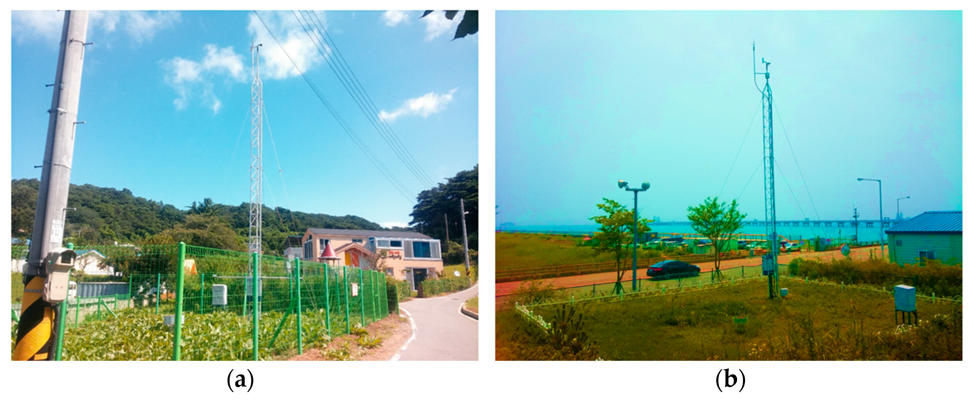
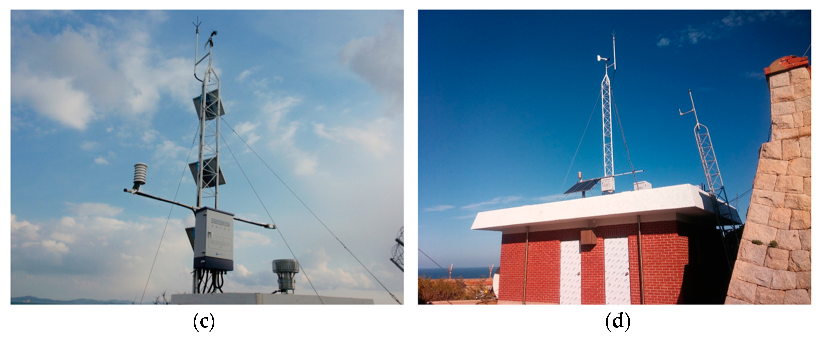
Figure 1 shows the equipment installed at all four sites used to measure wind speed and direction. A cup-type anemometer and anemoscope are installed on each vertical tower to measure wind speed and direction. Apart from wind conditions, sensors are also installed in these vertical towers to record other weather conditions, such as temperature and humidity.

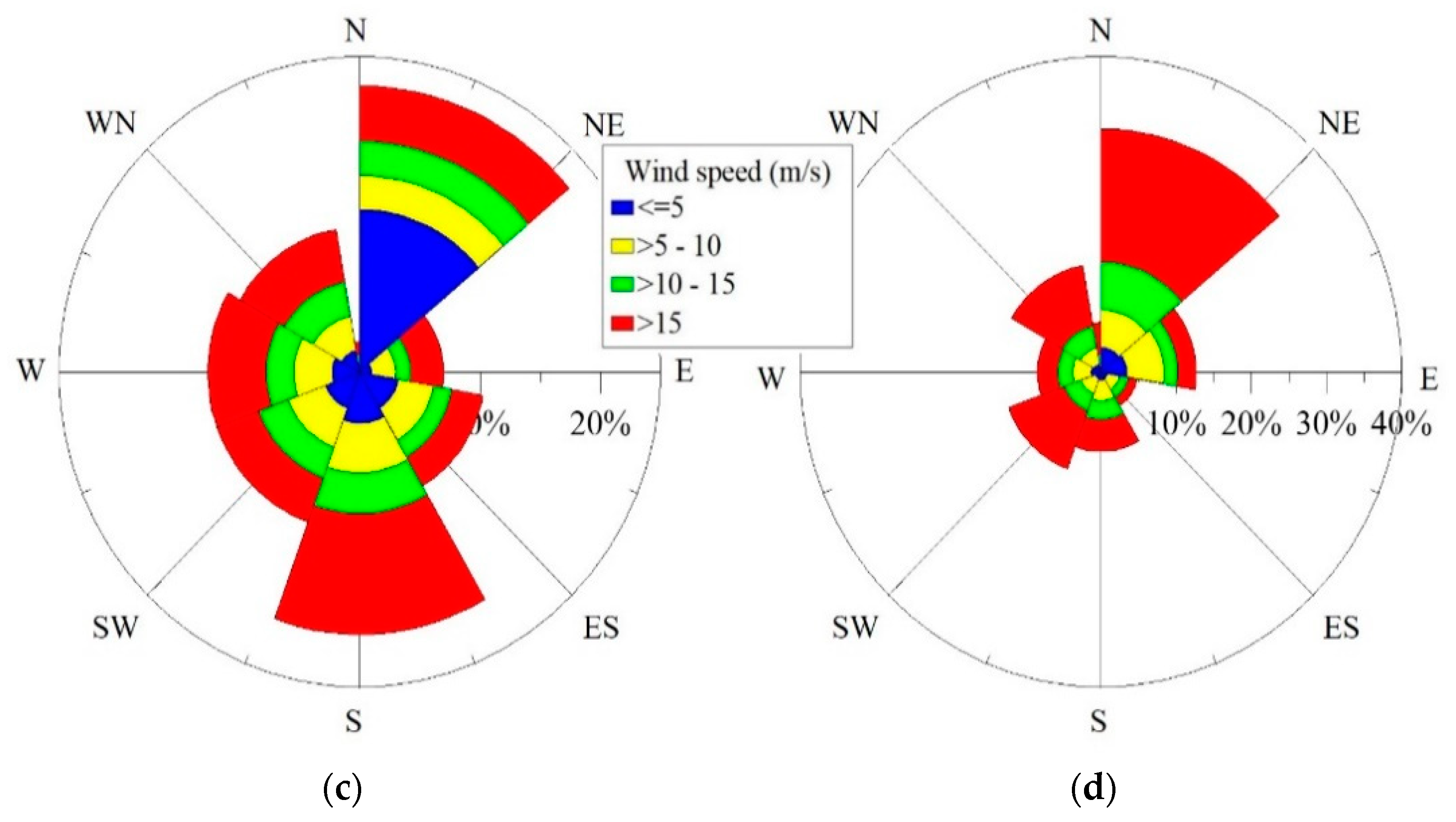
In order to provide a reference of wind speed strength and conditions at all four sites, Figure 2 has been prepared. These images (wind roses) show the wind direction and potential at a particular site for the total period. As can be observed in the wind rose diagrams, wind speed strength increases with height. The more wind speed strength there is, the more difficult it becomes to accurately measure and predict wind speed due to large fluctuations around the mean value. Therefore, it will be interesting to know which method, out of the six methods, predicts the wind speed at 60 m height with the most accuracy. Northeast is the prevailing wind direction at all sites except the 20 m height site.

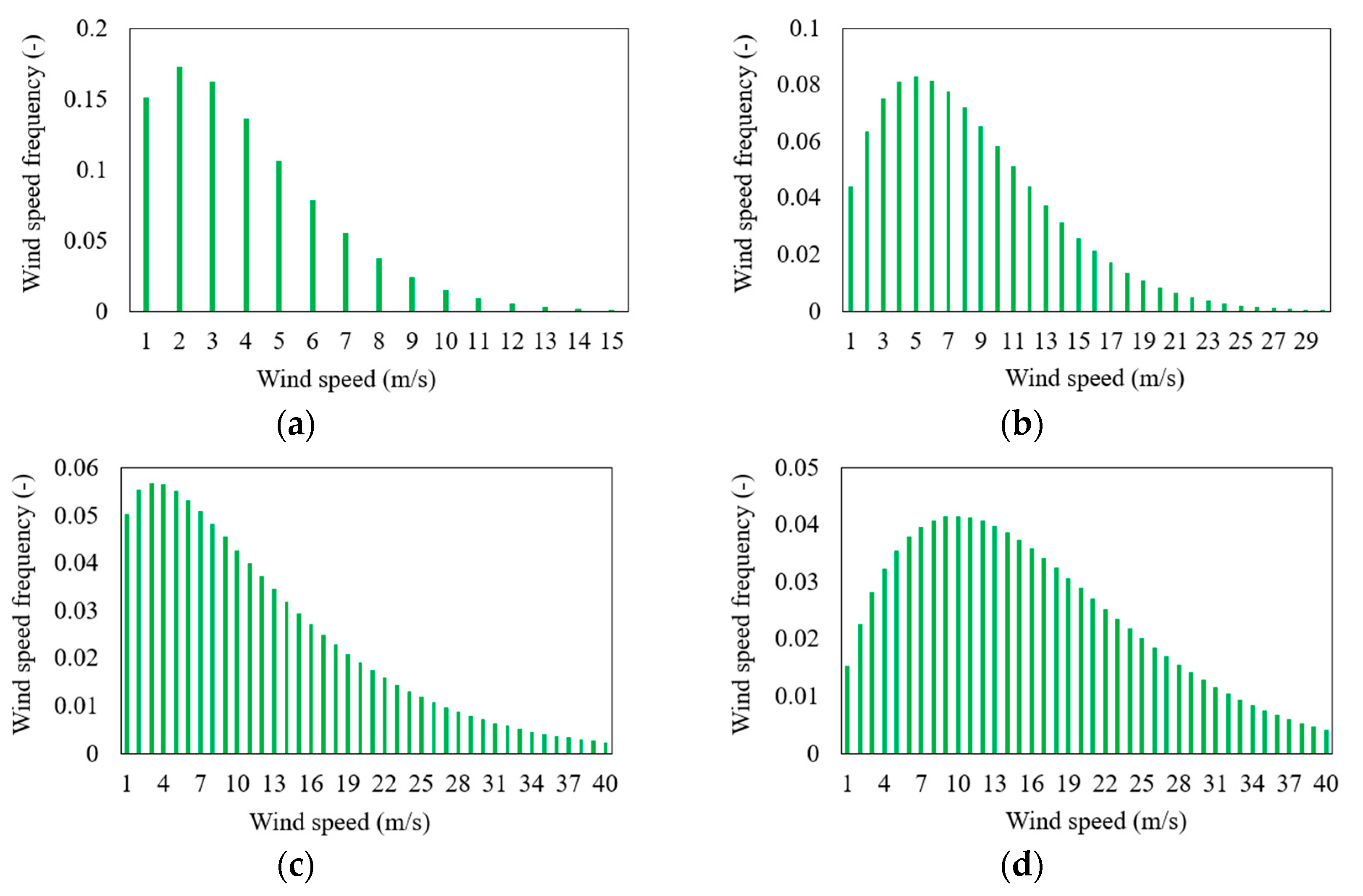
Figure 3 shows the frequency of different wind speed bins at all four sites for six years. The wind speed frequency at the four sites is nearly a perfect Weibull probability density function curve with different Weibull shape and scale parameters. The greater the resemblance between the measured wind speed frequency and the predicted wind speed frequency by the Weibull function, the more accurate results can be predicted by the Weibull algorithm. The magnitude of the most frequent wind speed increases with height as it is 2 m/s at a 10 m height, whereas it is 5, 5, and 10 m/s in the case of 20, 30, and 60 m heights, respectively. The total number of wind speed bins also increases with anemometer height, requiring more computational time and cost to predict the wind data using the Weibull algorithm.

2.3. Error Estimation in Weibull Parameter Prediction Models

The accuracy of the six methods in determining Weibull parameters cannot be directly evaluated. For this purpose, wind potential indicators such as mean wind speed, wind power density (WPD), and wind speed frequency are estimated using the Weibull parameters k and c. Then, the same terms are also calculated using real-time measured wind data, and both values are compared to determine the relative error. Wind potential indicators should be chosen to be determined in both cases, i.e., measured wind data and Weibull-predicted wind data.

The mean wind speed ($\overline{v})$ measured, predicted by Weibull and absolute relative error in a specific Weibull method, can be defined mathematically as shown in Equations (13)–(15).

$${\overline{v_{measured}}}_{}=\frac{1}{n}\left[{\sum }_{i=1}^n{v}_i\right]$$

(13)

$${\overline{v_{weibull}}}_{}=c\Gamma (1+1/k)$$

(14)

$$\left|{Error}_{\overline{v}}\right|=\left|\frac{{\overline{v_{measured}}}_{}-\overline{v_{weibull}}}{{\overline{v_{measured}}}_{}}\right|$$

(15)

The measured $WPD$ and that predicted by Weibull, as well as the absolute relative error in a specific Weibull method, can be defined mathematically as follows, in Equations (16)–(18).

$${WPD}_{measured}=\frac{1}{2}\rho \overline{{v_{real}}^3}$$

(16)

$${WPD}_{weibull}=\frac{1}{2}\rho c^3\Gamma (1+3/k)$$

(17)

$$\left|{Error}_{WPD}\right|=\left|\frac{{WPD}_{measured}-{WPD}_{weibull}}{{WPD}_{measured}}\right|$$

(18)

Wind speed frequency ($f)$ is the probability of occurrence of a specific wind speed bin in a time-series-based wind data set. Both measured wind data and wind data sets predicted by the Weibull algorithm can be used. In order to assess the accuracy performance of each of the six methods in predicting the wind speed frequency, three different error terms are introduced. These error-indicating terms are MABE, RMSE, and R. Each of these error terms can be mathematically defined as follows in Equations (19)–(21).

$${MABE}_f=\frac{1}{n}{\sum }_{i=1}^n\left|f_{i,measured}-f_{i,weibull}\right|$$

(19)

$${RMSE}_f=\sqrt{\frac{1}{n}{\sum }_{i=1}^n{\left(f_{i,measured}-f_{i,weibull}\right)}^2}$$

(20)

$$R_f=\frac{\sum _{i=1}^n{\left(f_{i,weibull}-\overline{f_{weibull}}\right)\left(f_{i,measured}-\overline{f_{measured}}\right)}^{}}{\sqrt{\left[\sum _{i=1}^n{\left(f_{i,weibull}-\overline{f_{weibull}}\right)}^2\right]\left[\sum _{i=1}^n{\left(f_{i,measured}-\overline{f_{measured}}\right)}^2\right]}}$$

(21)

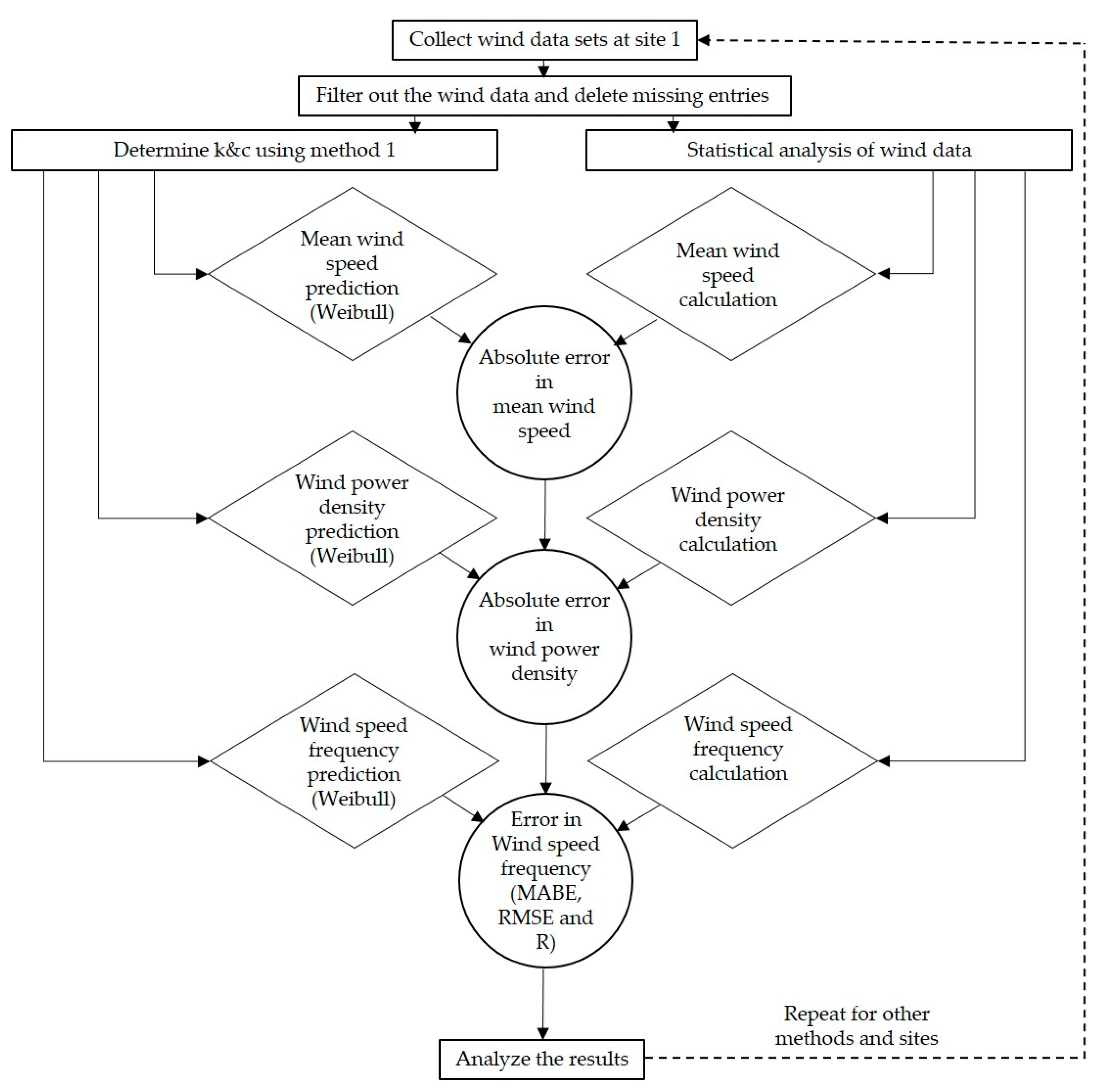
Figure 4 describes the overall process of evaluating the accuracy performance of each of the six methods for all four sites where wind data are measured at different heights.

3. Analysis and Results

3.1. Mean Wind Speed

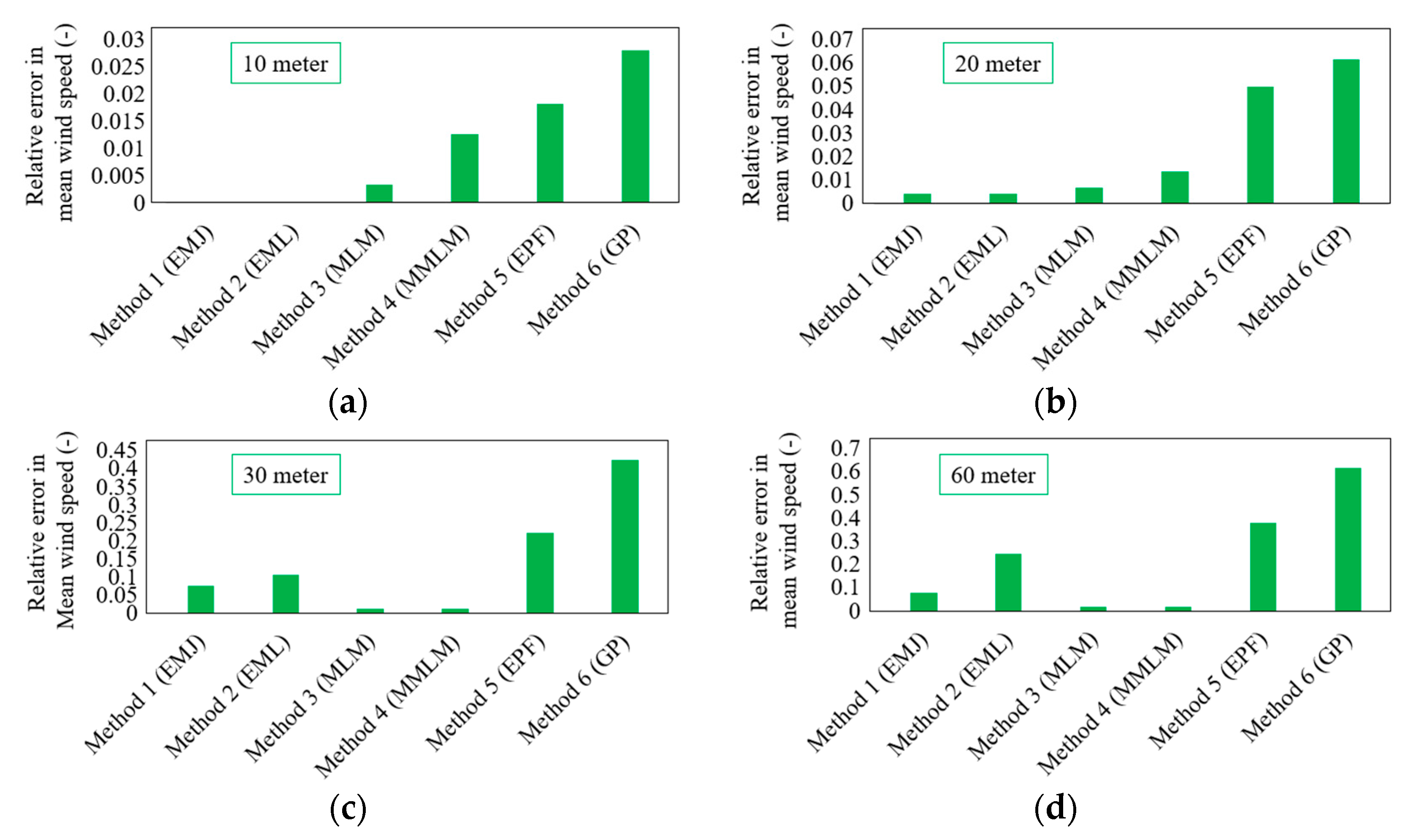
Mean wind speed is one of the most basic and few parameters that can be determined through measured and Weibull-predicted wind data sets. The Weibull mean wind speed is not directly calculated but determined through Weibull shape and scale parameters. Figure 5 shows the absolute magnitude of relative error between two mean wind speeds, i.e., calculated by measured wind speed and estimated by the Weibull algorithm. Equation (15) shows the exact definition of error in mean wind speed.

Two important and distinct phenomena can be observed in Figure 5. The first one is the effect of wind data height on the accuracy of the results, and the second is the relevance of each method at different wind data heights. No single method is the most accurate at any wind data height. At low heights (10 and 20 m), the EPF and GP methods show the worst accuracy performance, whereas the EMJ and EML are the optimum choices. Meanwhile, at medium and large wind data heights (30 and 60 m), the MLM and MMLM show the least error in mean wind speed. Like low wind data heights, the EPF and GP methods again show the worst accuracy performance at medium and large wind data heights, respectively.

The accuracy performance of each of the six methods is largely due to the type of internal algorithm and mathematical approximations used to estimate the mean wind speed. For example, due to relatively simple algorithms with less complexity and the straightforward nature of the EMJ and EML (as described in Section 2.1.1 and Section 2.1.2, respectively), these methods are the best fit for wind data measured at low heights where fluctuations in the wind speed are not that high. As the wind data height increases, these two methods (EMJ and EML) become less effective because of the less robust algorithm. However, for the medium and large wind data heights (30 and 60 m), the MLM and MMLM are the best fit because of the robust and thorough iterative process used to reach the final results (as described in Section 2.1.3 and Section 2.1.4, respectively). The choice of each method also depends on the computational time and resource availability. Although the EMJ and EML are computationally cheaper than the MLM and MMLM, the accuracy of the predicted results is also one of the main criteria that should be considered while selecting a specific Weibull method to predict the wind data at a specific site. The EPF and GP methods show the worst performance in the present scenario, as also stated by Kidmo et al. [6] and Chang [7], respectively. The EPF method is a simple approximation method that cannot handle complex data sets. Similarly, the GP method uses graphical approximation, which makes it very hard to match accurately for different types of wind data sets collected at different heights and in different complex terrains.

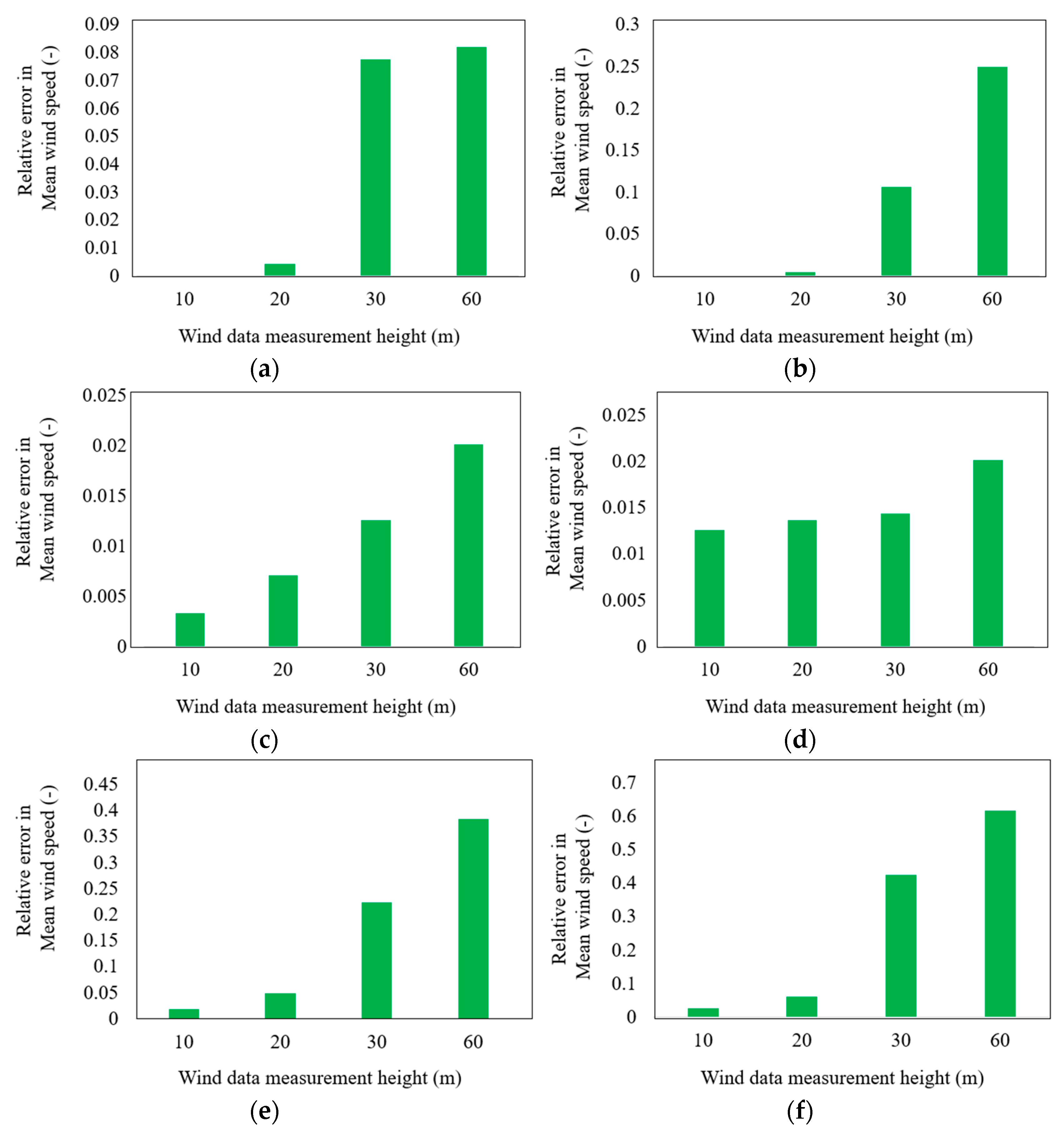
Figure 6 shows the absolute relative error in mean wind speed for each of the six Weibull methods according to the wind data measurement height. Generally, the amount of error increases linearly with height for all six methods. However, the magnitude of error is quite different in different scenarios. The EMJ and EML are quite effective at low wind data heights, whereas the MLM and MMLM show superior accuracy performance at medium and large heights. For example, at a 60 m wind data height, the mean wind speed, as predicted by the EMJ, has a relative deviation of 8% from the actual mean wind speed. In contrast, this difference is quite low in the MLM and MMLM, corresponding to nearly 2%. On the other hand, at a 20 m wind data height, the lowest error is produced by the EML (nearly 0.1%), whereas at the same height, the MLM and MMLM produce error magnitudes of 0.75% and 1.4%, respectively. Therefore, the choice of the Weibull parameter prediction method largely depends on the wind data height, and this process should be carefully adapted to obtain accurate results.

3.2. Wind Power Density

Wind resource availability at a potential site can be assessed using the WPD. The energy available at the site for conversion by a wind turbine is indicated by the WPD, expressed in watts per square meter. A site’s WPD is another factor that can be used to compare and choose the best sites for wind turbines and vice versa. Wind turbines placed at sites with higher WPDs typically produce more electricity. Therefore, it is very important to estimate the WPD of a site accurately for more efficient wind turbine selection and power production.

Table 2. Error in WPD.

	WPD (Watt/m2)							Absolute Relative Difference in WPD (%)
Height (m)	Measured	EMJ	EML	MLM	MMLM	EPF	GP	EMJ	EML	MLM	MMLM	EPF	GP
10	1.58	1.59	1.57	1.56	1.56	1.54	1.53	0.15	0.57	1.28	1.57	2.97	3.21
20	14.00	14.21	13.60	13.59	13.57	13.43	13.36	1.52	2.88	2.92	3.07	4.10	4.62
30	159.04	154.02	153.48	163.76	163.96	165.81	166.62	3.15	3.50	2.97	3.09	4.26	4.77
60	253.78	264.50	265.75	261.94	263.21	267.03	269.65	4.23	4.72	3.22	3.72	5.22	6.25

shows the absolute difference between the actual or measured WPD and those estimated by all six methods. The wind power values computed using the six Weibull distributional approaches and those produced using data on measured wind speed are first described. For this purpose, some significant descriptive statistics are first calculated for the four stations under examination, including minimum, maximum, and mean values, standard deviation, and range of values. The distribution of the WPD computed using six different approaches and those computed using measured wind speed data can be compared using this analysis.

It is noted that the descriptive statistics of the WPD computed using the EMJ and EML are closer to the wind power calculated by observed data at low wind data heights. The descriptive statistics of the WPD obtained by the MLM and MMLM are substantially closer to the wind power calculated by the measured data at medium and large wind data heights. It is important to note that the parameter k is calculated using the same equation in both approaches and that the only difference in the computation of the parameter c is why the descriptive statistics of the EMJ and EML methods are so similar. The error analysis conclusions drawn from the analysis of WPD are consistent with the mean wind speed error results.

Therefore, when the MLM and MMLM are being used to calculate the Weibull parameters, a better distributional fitting between the estimated WPD by the Weibull function and that calculated by measured wind data would be achieved for medium and large wind data height sites. At the same time, more precise fitting curves are obtained for the stations with low wind data heights when the EMJ and EML are used to calculate the Weibull parameters. Notably, when the GP and EPF methods are used to determine the k and c parameters, the biggest distributional disparities between the WPD calculated by observed data and that derived by the Weibull function are produced.

3.3. Wind Speed Frequency

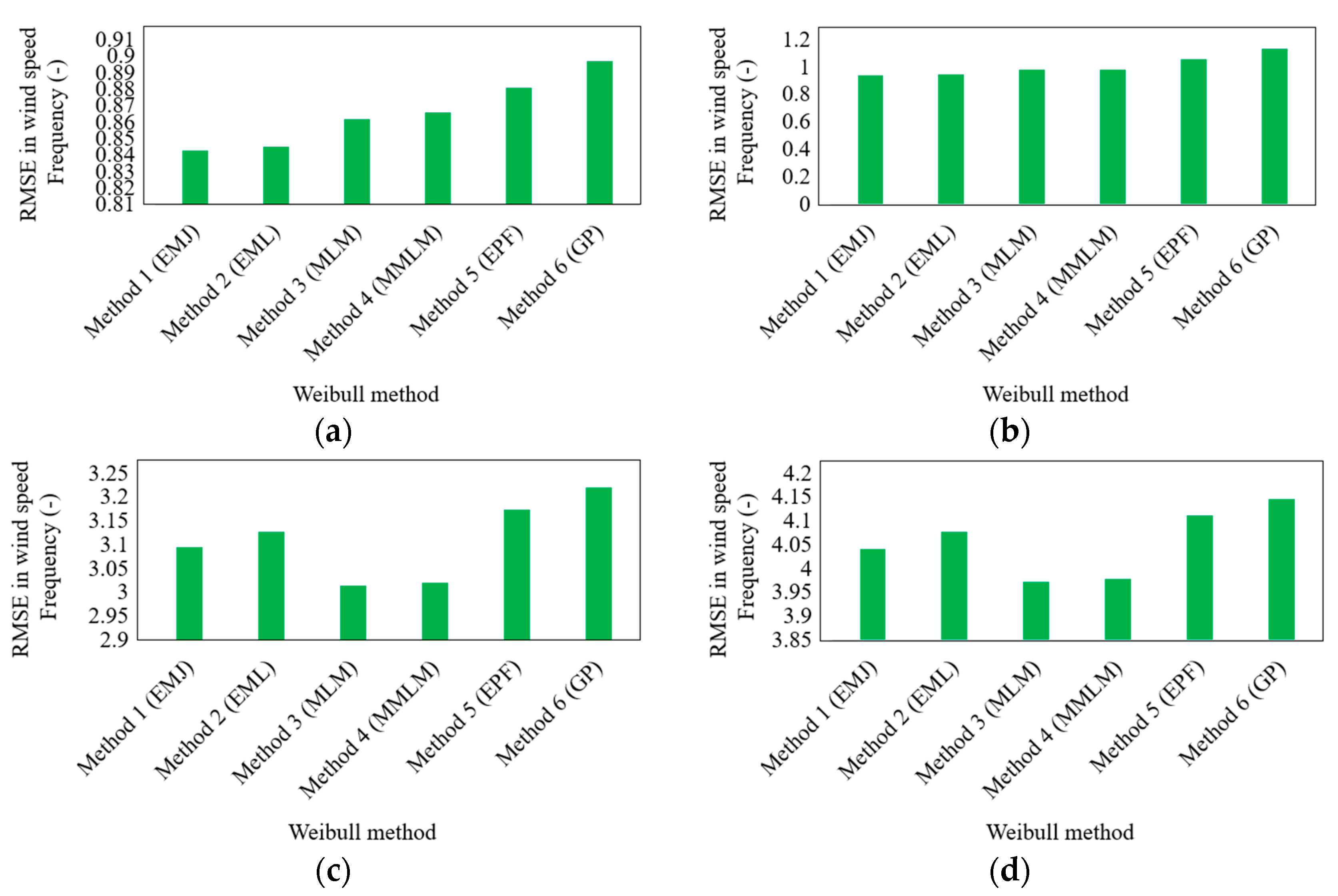
Even though the presented descriptive statistics provide insightful statistical information, particularly regarding the distribution of the WPD, they cannot be used exclusively to assess the level of precision of the six methods for calculating parameters such as wind speed frequency. As a result, the six selected parameter estimation methods are evaluated using the statistical indicators described in Section 2.3. 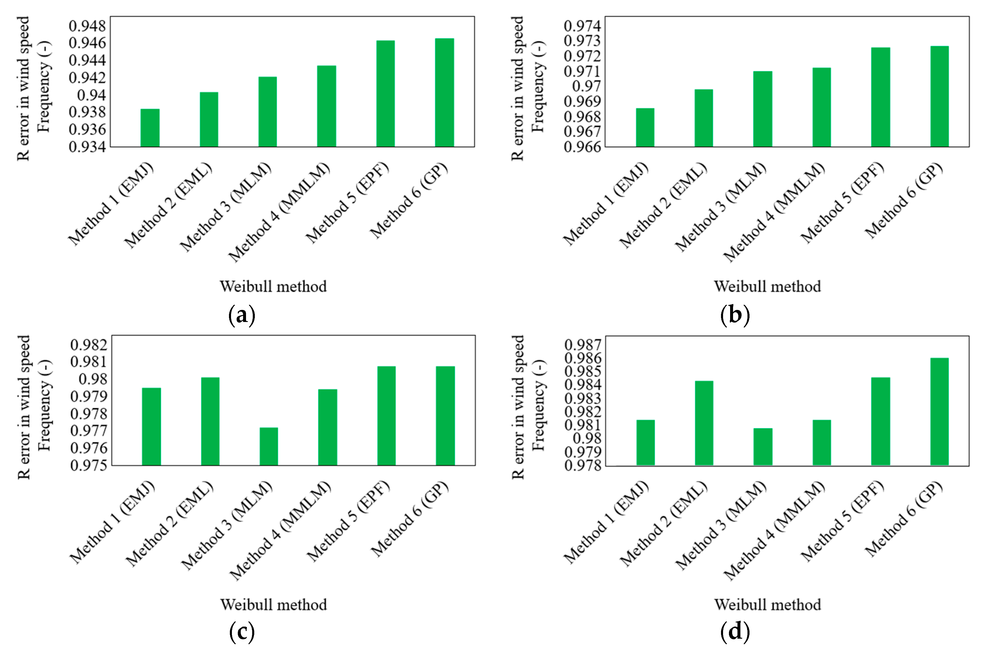The performance evaluation results of the six chosen methods are shown in Figure 7, Figure 8 and Figure 9 regarding MABE, RMSE, and R error for each of the four sites.

It is important to mention that each statistical parameter, i.e., MABE, RMSE, and R error, offers several helpful perspectives to contrast the approaches. In order to examine the disparities between the calculated wind power by observed data and that of the Weibull density function within different viewpoints with much higher confidence, all of these statistical indicators have been combined. The findings demonstrate that when the parameter estimation methods are altered, the computed wind speed frequency values lose accuracy. The calculated wind speed frequency values by the Weibull density function are in good agreement with the wind speed frequency values computed by the observed wind data for all four stations when the four methods of EMJ, EML, MLM, and MMLM are employed to compute the Weibull parameters at low and large wind data heights, respectively, as also concluded in previous sections.

Due to the low values of error terms (such as MABE and RMSE) and high values of R, this conclusion has been reached. On the other hand, it has been discovered that when the GP and EPF approaches are used to determine the k and c parameters, the lowest agreements are reached. The EMJ or EML is most effective for determining the wind speed frequency for two stations (10 and 20 m wind data height), according to the statistical findings of Figure 7, Figure 8 and Figure 9, when the k and c parameters are computed. The MLM or MMLM approach yields the most accurate wind speed frequency results for stations with medium or large wind data heights.

3.4. Temporal Wind Speed Series

The accuracy results presented here are based on full-period data sets of six years (2015–2020) for all sites. Although the mean values of wind speed and WPD can also lead to conclusive results, time-dependent wind data error results can increase confidence in selecting a suitable Weibull method for any given wind data site. Time-series wind error results are also important because they can help suggest a minimum and suitable number of wind data measurements required to accurately analyze the wind potential at a site. At some sites, the numbers of measured wind data are very small, which offers a great challenge for wind farm developers and researchers to choose an appropriate Weibull method according to the local availability of several wind data sets.

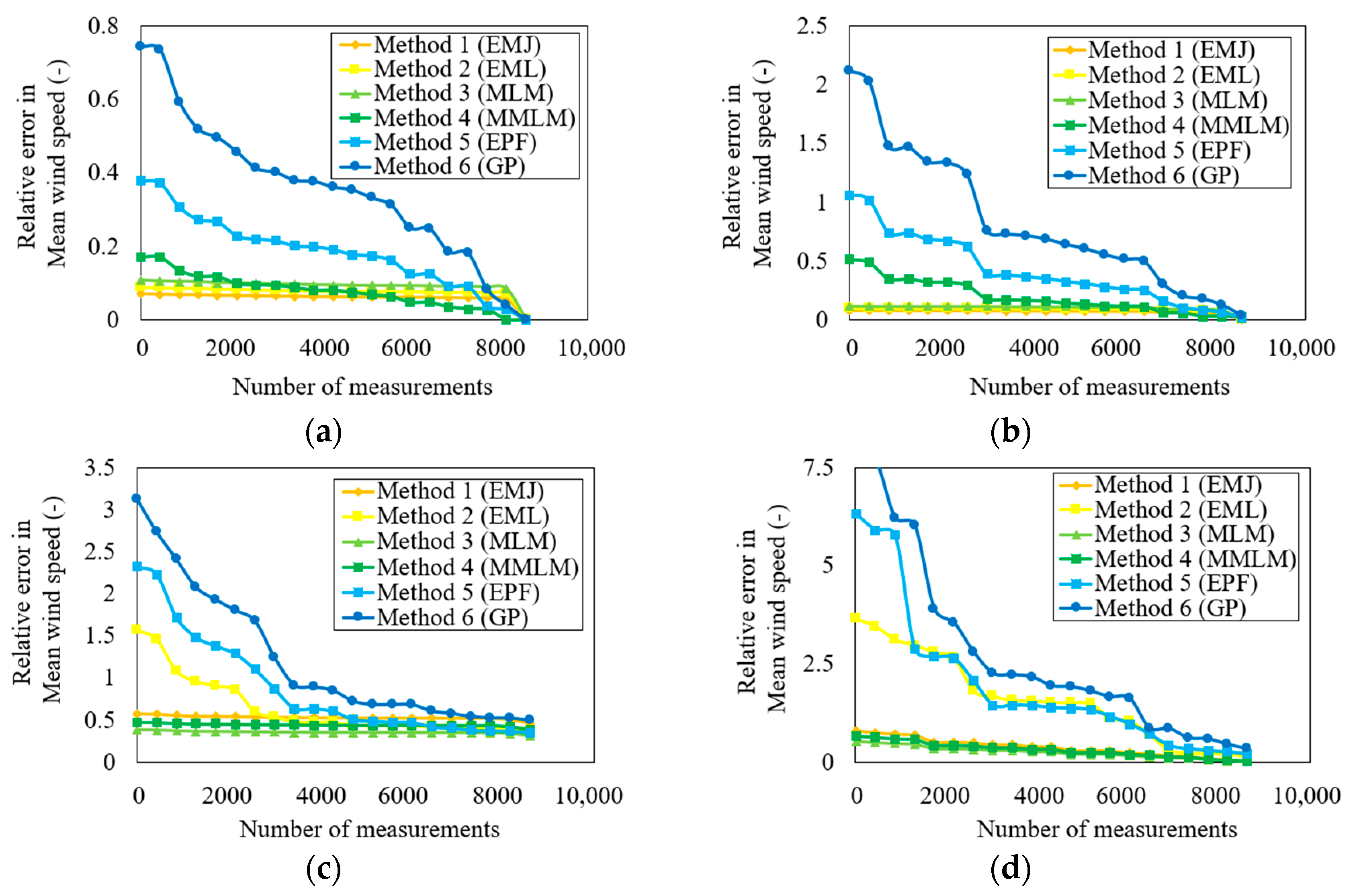
Figure 10 shows the relative error in mean wind speed according to several measured wind data using all six methods at four sites. In order to make calculations easy and understandable, a sample of wind data from one year on an hourly basis is selected from all sites. In Figure 10, each wind data point represents the average values during one hour of wind data measurements, and it is assumed that wind characteristics remain the same during that hour. One general phenomenon that can be observed in all graphs of Figure 10 is that the relative error in mean wind speed is on the downfall as the number of wind data measurements increases for all methods and sites. The second point to be noted is that the GP method yields the maximum amount of error in mean wind speed estimation. This conclusion is in line with previous observations established in the present study. The third observation that is very clear in Figure 10 is the magnitude of relative error increase with wind data height for all six methods. The fourth noticeable conclusion that can be drawn from Figure 10 is that after almost 8000 wind data measurements, the relative error in mean wind speed is so significantly low that it can be ignored for all wind data heights and methods considered in the present study. From Figure 10, it can be concluded that the EMJ and EML are best suited for sites with wind data measured at low heights and vice versa for the MLM and MMLM at large wind data heights. The last-mentioned point matches the conclusions drawn previously in the present study very well.

It should be noted that the total number of days for analysis is fixed at 2130 because six years’ worth of wind speed data were used in this study to calculate daily WPD (determined after data filter analysis). The actual total number of effective wind data availability days is different for each site, i.e., it is 2139 for site 1 (10 m), 2145 for site 2 (20 m), 2151 for site 3 (30 m), and 2146 for site 4 (60 m). According to the time-series analysis criterion, the results of earlier statistical indicators and previous time-series analyses are highly coherent. The EMJ or EML approach produces the best results for two stations with low wind data measurement height, according to statistical findings of Figure 10 when used to compute the k and c parameters. At the same time, the MLM or MMLM approach provides more accuracy for places with medium to large wind data heights.

4. Discussion

The variance in regional wind characteristics may cause the more effective strategy to differ for each place. Figure 2 and Figure 3 show that the magnitude of mean wind speeds is noticeably higher at site 4 than at site 1, which is one of the key distinctions in the wind characteristics. It could explain why the MLM or MMLM approach worked better for sites 3 and 4 (particularly for site 4), whereas the EMJ or EML performed better for sites 1 and 2. Future studies might examine this topic in more detail. It is also crucial to note that all statistical indicators show that the EMJ and EML work similarly. However, with a small difference, the EMJ approach achieves a better level of accuracy. Each table shows the most precise approach for each place in bold. The GP and EPF methods, which have quite large differences compared to other chosen ways, rank in the final two sites as the weakest methods (methods with the largest error), meaning that their use results in significantly more errors than other methods.

Although each region has unique wind power characteristics, it is important to note that the obtained results regarding the effectiveness of the approaches for estimating the parameters of the Weibull distribution function can be applied to regions with similar wind distributions. The results can only be generalized to areas with comparable wind power characteristics. It is also observed that for all stations, the c parameter values from all approaches are very similar, with the GP method showing the largest differences overall. Nevertheless, the k parameter values for the EMJ, EML, MLM, and MMLM are consistent over all months, whereas the k values for the GP and EPF methods are larger than those of the other methods. The calculated values of WPD fluctuate significantly more due to these variations in the k and c values for these approaches. Accurately estimating Weibull parameters is one of the most important aspects of wind energy potential estimating algorithms and software. The present study provides basic guidelines for choosing an appropriate method for estimating Weibull parameters according to wind data height. The results of the present study have been formulated through a robust error analysis. The results of the present study can also be used in interpolation for wind data heights in between or higher than what is presented in the present study. It is worth mentioning that the characteristics of a site terrain do not have any effects on the presented results because the wind data used in our study were measured experimentally, which already incorporates the site-specific parameters such as surface roughness, wind shear, etc.

5. Conclusions

The present study evaluates the accuracy performance of six different numerical methods used to estimate Weibull shape and scale parameters. The six considered methods are the empirical method of Justus (method 1), the empirical method of Lysen (method 2), the maximum likelihood method (method 3), the modified maximum likelihood method (method 4), the energy pattern factor method (method 5), and the graphical method (method 6). The accuracy performance of each method is evaluated for different heights of measured wind data categorized as low, medium, and high.

The analysis of mean wind speed, wind power density, wind speed frequency, and temporal wind series showed that methods 1 and 2 are the most accurate for low and medium wind data heights. Methods are simple mathematical tools that can only produce accurate results for low-wind-speed prediction but fail to produce the most accurate results at high wind speed. Methods 3 and 4 produced the most accurate results when applied to wind data measured at relatively larger heights (60 m). Although both methods are quite robust and iterative numerical algorithms that can produce accurate results for high-wind-speed prediction, the computational time is also increased. Methods 5 and 6 are the least suitable methods for wind energy analysis using the Weibull algorithm, as the error is maximum in predicted mean wind speed, wind power density, and wind speed frequency at all studied wind data heights.

The minimum relative error in mean wind speed is 0.01% at a 10 m height for method 1, whereas its maximum value is 61% at a 60 m height for method 6. Similarly, the minimum and maximum values of relative error in WPD are 0.15% (10 m, method 1) and 6.25% (60 m, method 6), respectively. Wind speed frequency prediction also shows a similar pattern with a minimum and maximum error occurring using method 1 and method 6, respectively. For all methods and heights, the absolute relative error in mean wind speed tends to lower significantly with several wind speed measurements.