An Adaptive Modeling Method for the Prognostics of Lithium-Ion Batteries on Capacity Degradation and Regeneration

Abstract

Accurate prediction of remaining useful life (RUL) is crucial to the safety and reliability of the lithium-ion battery management system (BMS). However, the performance of a lithium-ion battery deteriorates nonlinearly and is heavily affected by capacity-regeneration phenomena during practical usage, which makes battery RUL prediction challenging. In this paper, a rest-time-based regeneration-phenomena-detection module is proposed and incorporated into the Coulombic efficiency-based degradation model. The model is estimated with the particle filter method to deal with the nonlinear uncertainty during the degradation and regeneration process. The discrete regeneration-detection results should be reflected by the model state instead of the model parameters during the particle filter-estimation process. To decouple the model state and model parameters during the estimation process, a dual-particle filtering estimation framework is proposed to update the model parameters and model state, respectively. A kernel smoothing method is adopted to further smooth the evolution of the model parameters, and the regeneration effects are imposed on the model states during the updating. Our proposed model and the dual-estimation framework were verified with the NASA battery datasets. The experimental results demonstrate that our proposed method is capable of modeling capacity-regeneration phenomena and provides a good RUL-prediction performance for lithium-ion batteries.

1. Introduction

The successful applications of lithium-ion batteries in portable electronics, medical devices, electric vehicles, and space systems have stimulated lithium-ion batteries being the primary energy storage devices in more and more areas. The market for lithium-ion batteries has expanded dramatically over the past few decades due to their high energy/power density, low self-discharge, and environmental friendliness [1,2,3,4]. The monitoring and prognostics of lithium-ion batteries play a critical role in guaranteeing their safe and reliable usage. The state of health (SOH) is one of the key indicators to quantify the health state of a working battery when contrasted with its initial capability, and the remaining useful life (RUL) is extracted according to the SOH. The performance of the active material and electrolytes inside the battery reflects the battery health, and the deterioration of the performance will lead to the degradation of the battery’s internal health state [5]. Fast identification of the SOH is critical for working batteries to avoid unexpected failures. A reliable estimation of the SOH or RUL is helpful for early warning in case of battery failure, and a proper maintenance strategy or battery replacement scheduling can be prepared in advance when the battery SOH is understood well. However, accurate prediction of the RUL is challenging, which involves nonlinear degradation and regeneration phenomena. In this paper, we focus on modeling the battery degradation and regeneration phenomena for RUL prediction.

2. Related Work

2.1. Battery Degradation

Battery degradation is the process by which battery performance gradually deteriorates until the battery fails to provide enough power for electric systems. The degradation process is very complicated, and the health indicator (HI) is usually employed to characterize this degradation process for simplicity. The RUL is defined as the remaining cycles before the HI deteriorates to an unacceptable threshold. As the lithium-ion battery ages, the impedance will increase, and the fully charged capacity in each cycle will fade. Thus, the HI can be described by the impedance or capacity [6]. Some studies [7,8] regard the impedance as the HI. However, the measurement of the impedance often requires electrochemical impedance spectroscopy (EIS) measurements to collect complex impedance spectra, which is unavailable for an onboard implementation due to the sophisticated instrumentation and low efficiency in the measurement [6]. The most popular HI is the capacity, which is adopted by many studies [9,10,11]. This paper focuses on modeling the capacity depletion to predict the RUL of lithium-ion batteries.

The prognostics model for RUL prediction can be roughly classified into three categories (i.e., the mechanism model or physics-of-failure model, empirical model, and data-driven model). The physics-of-failure model [12] aims to model the capacity depletion by capturing the electrochemical process. The electrochemical process is very complicated and modeled by many mathematical equations, like partial differential equations, with many unknown parameters. Although the mechanism model has the potential to be accurate, the heavy computation for model identification is inappropriate for online RUL prediction [9].

Another popular model for RUL prediction is the data-driven model. Numerous data-driven models, for example naive Bayes [9], artificial neural networks [6,13], the Gaussian process regression model [8,14], and their combinations [15], have been utilized in the prognostics and health management of lithium-ion batteries. The data-driven model regards the battery aging process as a black box and does not require domain knowledge. The only requirements are the historical HI data or operating parameters during the battery’s degradation. The prognostics performance is highly dependent on the quality and the quantity of the data. However, the battery degradation data collected in the electrochemical degradation process are non-static and non-stationary, which makes it difficult for the data-driven model to predict.

A new trend is to fuse the data-driven model with the battery degradation properties. Ref. [16] proposed a nonlinear autoregressive (AR) model based on the analysis of the battery degradation process. The nonlinear AR model can be regarded as an empirical model, which is suggested by the properties of the HI data. Current studies for RUL prediction mainly focus on developing computationally efficient real-time methods, and the empirical model has been received increasing attention for RUL prediction. In contrast to the mechanism model, empirical models are concise, and the model parameters are adaptable to compensate for the model’s simplicity [10,17]. In addition, empirical models incorporate the battery degradation characteristics and relax the strict constraints on the data requirements as assumed in data-driven models. The filtering methods, such as the extended Kalman filter (EKF) [18] and the particle filter (PF) [10,19] are utilized to update the model parameters. The model-based filtering method incorporates the characteristics of both the battery degradation process and the Bayesian inference methods to deal with uncertainties, which is more efficient and accurate for the real-time prognostics of lithium-ion battery systems [20].

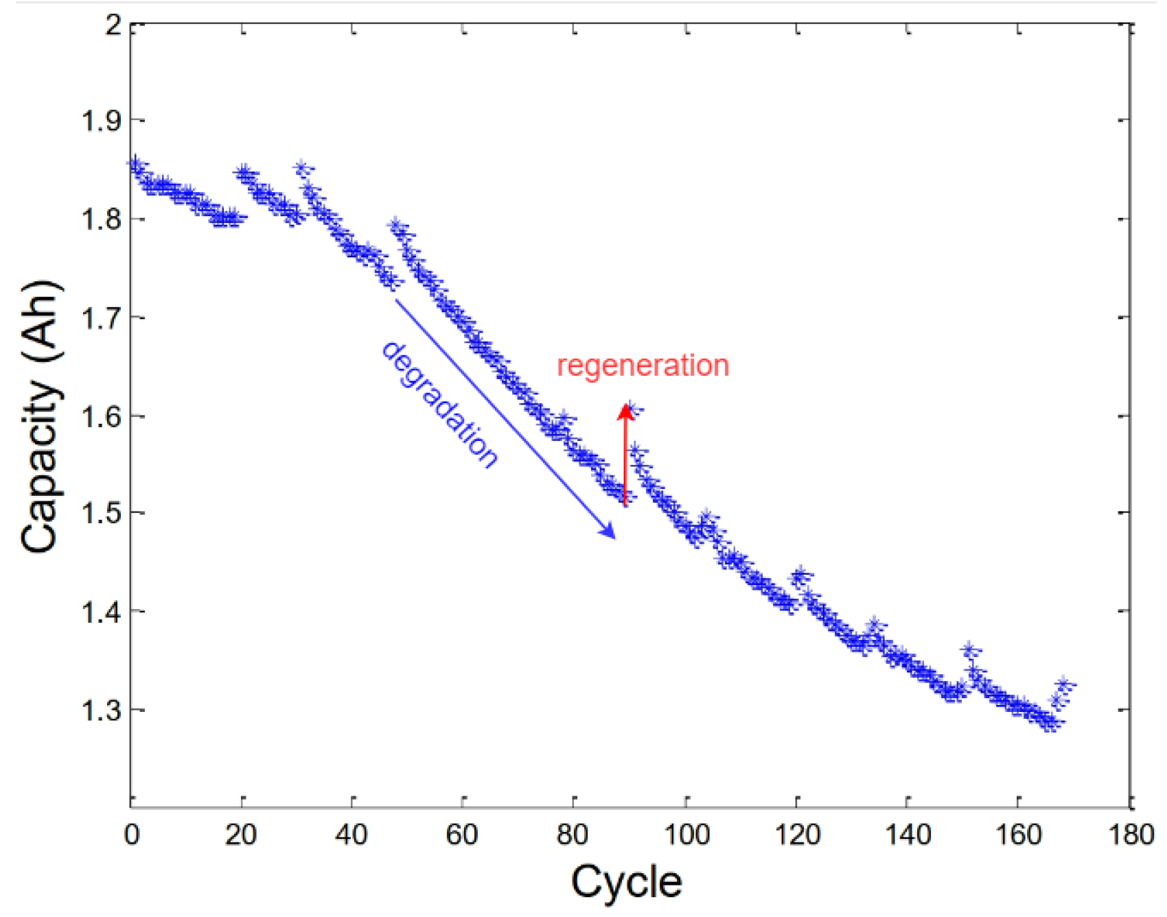
2.2. Regeneration Phenomenon

Accelerated aging experiments for lithium-ion batteries have inevitably introduced some inconsistent conditions among the repeated charge/discharge cycles. For example, the period between the end of the previous fully discharged process and the beginning of the next charge process may be different. We regard the period when the battery is not being charged or discharged as the rest time, which widely exists in the practical usage of batteries. The regeneration phenomenon happens when the period between two adjacent charge/discharge cycles is long enough [21]. As shown in Figure 1, the capacity suffers sudden increases in some cycles. In practice, the rest status takes up a large amount of the battery life, and the increase in capacity can prolong its service life. It would be an enormous waste to replace the battery early due to the failure consideration of the regeneration phenomenon.

The regeneration phenomenon has been considered to be a self-recharge process and approximated with an exponential function [19,22]. Combined with the Coulombic efficiency as an adaptive parameter, the next charge/discharge cycle of capacity can be denoted by Equation (1).

$$C_{k+1}={\eta }_C{C}_k+{\beta }_{1}exp(-{\beta }_2/▵t_k),$$

(1)

where the fully charged capacity at the kth cycle is denoted as $C_k$, $▵t_k$ is the rest time, ${\eta }_C$ is the Coulombic efficiency, and ${\beta }_1$ and ${\beta }_2$ are model parameters to be estimated. The exponential model can slightly improve the RUL prediction performance during the regeneration and has been used by some studies [23,24] to cope with regeneration phenomena. However, this model regards the regeneration phenomenon happening in every cycle without any detection. Therefore, some researchers [25,26] propose detection modules to detect the capacity-regeneration phenomena. The detection results, as shown in Equation (2), can be incorporated into the state space model, as shown in Equations (3) and (4).

$$U_k=\left\{\begin{array}{cc}0,\hfill & \mathrm{if}\mathrm{no}\mathrm{self}\text{-}\mathrm{charge};\hfill \\ 1,\hfill & \mathrm{if}\mathrm{either}\mathrm{self}\text{-}\mathrm{charge}\mathrm{is}\mathrm{detected}\mathrm{at}\mathrm{cycle}\mathrm{k},\hfill \\ \hfill & \mathrm{or}\mathrm{self}\text{-}\mathrm{recharge}\mathrm{phenomenon}\mathrm{is}\mathrm{fading};\hfill \\ 2,\hfill & \mathrm{if}\mathrm{additional}\mathrm{self}\text{-}\mathrm{recharge}\mathrm{phenomena}\hfill \\ \hfill & \mathrm{are}\mathrm{detected}\mathrm{before}\mathrm{the}\mathrm{least}\mathrm{one}\mathrm{fades}.\hfill \end{array}\right.$$

(2)

State transition model:

$$\left\{\begin{array}{cc}\hfill & x_{1,k+1}={\alpha }_1{x}_{1,k}+{\omega }_{1,k},\hfill \\ \hfill & x_{2,k+1}={\alpha }_2{x}_{2,k}+\beta U_k+{\omega }_{2,k}.\hfill \end{array}\right.$$

(3)

Measurement model:

$$y_k=x_{1,k}+x_{2,k}+{\nu }_k,$$

(4)

where $x_{1,k}$ and $x_{2,k}$ represent the hidden states in cycle k, $y_k$ denotes the observed measurements, ${\alpha }_1$, ${\alpha }_2$, and $\beta$ are the model parameters, and ${\omega }_{1,k}$, ${\omega }_{2,k}$, and ${\nu }_k$ are the process noise. However, the self-recharge and capacity regeneration are different [27]. Self-recharge may happen within several minutes of rest time while the capacity-regeneration phenomenon requires several hours of rest and is not sensitive to a short rest time [21]. The magnitude of the regenerated capacity has been modeled with the hyperbolic tangent function by incorporating the rest time, and the regeneration phenomenon is determined according to the difference between two adjacent cycles of the SOH. Equations (5) and (6) describe the detection rule for the regeneration phenomenon.

$$DH\left(k\right)=H(k+1)-H\left(k\right).$$

(5)

$$r\left(k\right)=\left\{\begin{array}{cc}1,\hfill & \hfill DH\left(k\right)<Th,\\ -1,\hfill & \hfill DH\left(k\right)\ge Th,\end{array}\right.$$

(6)

where $H(k+1)$ and $H\left(k\right)$ represent the SOH in cycles $k+1$ and k, respectively. $DH\left(k\right)$ denotes the difference of the SOH between cycle $k+1$ and cycle k; $Th$ is a specified threshold to determine whether regeneration happens or not; $r\left(k\right)=-1$ means the regeneration happens, and $r\left(k\right)=1$ means the opposite.

The detection methods avoid modeling the regeneration phenomenon at every cycle and capture the regeneration effects when they are detected, which is sensible compared to Saha’s model [19]. However, these detection methods cannot detect the regeneration phenomena in a multi-step ahead manner and are unsuitable for the prediction of the RUL. Some recent works like [28] utilize wavelet decomposition technology to identify the future capacity regeneration module. The work in [29,30] adopted the Mann–Whitney U test (PF-U) and Wilcoxon rank sum test, respectively, to detect the future capacity regeneration point (CRP) accordingly to the historical data. These works are purely based on the historical data and ignore the inconsistent data distribution of the training stage and the prediction stage during the accelerated aging experiments. As previously mentioned, the regeneration phenomena are largely due to the rest of the time during the aging experiments. Some other works [31] decouple capacity regeneration based on the rest time from global degradation. The capacity-regeneration region is modeled by an exponential function, and the global degradation is modeled by a hybrid model with both the relevance vector machine and gray model. Another work [22], also based on the future rest time conditions for the regeneration phenomena’s identification, proposed a two-term exponential model for both the global degradation and local capacity regeneration for RUL prediction. In this work, we follow the rest time conditions for the regeneration identification and incorporate the regeneration effects into the Coulombic efficiency-based degradation model for RUL prediction, which is straightforward, robust, and flexible for the dynamic degradation.

3. Model Development, Identification, and Prediction

Identifying the capacity regeneration and estimating it properly are critical to an accurate RUL prediction. We propose an explainable, accurate, and straightforward model based on the aforementioned models [19,25,26]. In order to cope with data uncertainties and improve the adaptability of our proposed model, the Bayesian Monte Carlo simulation method is used for model identification. The dual estimation and kernel smoothing are also incorporated. With the identified model and the expected regeneration-detection results, we can implement the multi-step-ahead prediction for the RUL.

3.1. Proposed Model

Instead of the fixed Coulombic efficiency (CE) in Saha’s model [19], we are convinced by Refs. [32,33] that the CE would evolve during the battery degradation process. Thus, we adapted the CE during the model identification. The proposed model consists of two components, as shown in Equation (7). The first term is the same as the first term of Saha’s model with a slightly different CE that can be adapted during the identification process. The second term is replaced with a regeneration-detection module, which allows for multi-step-ahead detection with the expected condition of rest time. The proposed model can be regarded as an auto-regressive model with an additional term. Whenever the regeneration happens, the capacity will increase not only in the current cycle, but also in the following cycles. The regeneration magnitude is assumed to be a constant in the beginning and can be learned during the model identification. In future cycles, the regeneration effects will decay gradually.

$$C_{k+1}=\alpha C_k+\beta U_{k+1},$$

(7)

where $C_k$ denotes the kth cycle of the charge capacity; $U_{k+1}$ is the detected regeneration results; $\alpha$ and $\beta$ are the parameters of the model, and both have physical meanings; $\alpha$ represents the CE without interfering with the regeneration phenomena; $\beta$ indicates the magnitude of capacity regeneration. We have presented the structure of our model in Equation (7) so far. In Appendix A, we prove that the structure of our model when ignoring the regeneration-detection part is equivalent to Olivares’s model [25]. However, our model only has one state and two model parameters, which is less complicated than the two states and three model parameters in Olivares’s model. Inspired by the strong relationship between the regeneration phenomenon and rest time [19,21,27], we identified the capacity regeneration according to the rest time. If the rest time is longer than a rated threshold, the regeneration phenomenon will be regarded as significant in the following cycles. On the condition of future steps’ rest time, we can detect the regeneration phenomena in advance. The detection rule is described by Equation (8).

$$U_{k+1}=\left\{\begin{array}{cc}0,\hfill & \hfill \mathrm{if}\delta t(k+1)<\mathrm{\Theta },\\ 1,\hfill & \hfill \mathrm{if}\delta t(k+1)\ge \mathrm{\Theta },\end{array}\right.$$

(8)

where $\delta t(k+1)$ is the rest time between cycle $k+1$ and cycle k, as shown in Equation (9), $\mathrm{\Theta }$ is the rated threshold, which indicates how long a rest period is to lead to an apparent regeneration phenomenon, and $\mathrm{\Theta }$ is a super-parameter.

$$\delta t(k+1)=T(k+1)-T\left(k\right),k=1,2,3,···,$$

(9)

where $T(k+1)$ and $T\left(k\right)$ are the chronological time when a battery finishes the $(k+1)$th and the kth cycle of charge and discharge, respectively.

3.2. Particle Filtering Method

The battery degradation process is a non-static, non-stationary, and nonlinear dynamic process. To capture these properties, we incorporated the particle filtering (PF) method to cope with the uncertainties in the non-stationary aging process. The PF method [34,35] reformulates the model under the Bayesian framework and utilizes a set of particles associated with weights to approximate the state probability density function (pdf). Particles are sampled from a prior estimation of the state pdf and propagated through the modeling process. The important weights of these particles are recursively updated by available measurement observations (capacity, in our case). However, the variance of these weights increases stochastically over time, which ends up with a few particles dominating the approximation of the state pdf and ignoring other particles [36]. This degeneracy phenomenon prevents the particle filter from being useful until the resampling stage has been included [34]. Model parameters can be assumed as another kind of state to be tracked. In order to use the PF framework, the state transition model and measurement model must be derived first. In our case, Equation (10) denotes the transition model of the parameters.

$$\left\{\begin{array}{cc}\hfill & \hfill {\alpha }_{k+1}={\alpha }_k+{ϵ}_{\alpha },{ϵ}_{\alpha }\sim N(0,{\sigma }_{\alpha }^2),\\ \hfill & \hfill {\beta }_{k+1}={\beta }_k+{ϵ}_{\beta },{ϵ}_{\beta }\sim N(0,{\sigma }_{\beta }^2).\end{array}\right.$$

(10)

We can reformulate our proposed model for the state transition model as Equation (11).

$$C_{k+1}={\alpha }_{k+1}{C}_k+{\beta }_{k+1}{U}_{k+1}+{ϵ}_C,{ϵ}_C\sim N(0,{\sigma }_C^2).$$

(11)

The capacity can be obtained from the measured signals, and we cast the measurement model as Equation (12).

$$\widetilde{C_k}=C_k+{ϵ}_m,{ϵ}_m\sim N(0,{\sigma }_m^2),$$

(12)

where $\widetilde{C_k}$ denotes the measured capacity; the noise $ϵ$ follows a Gaussian distribution with zero mean and ${\sigma }^2$ variance; other notations are the same as previous equations.

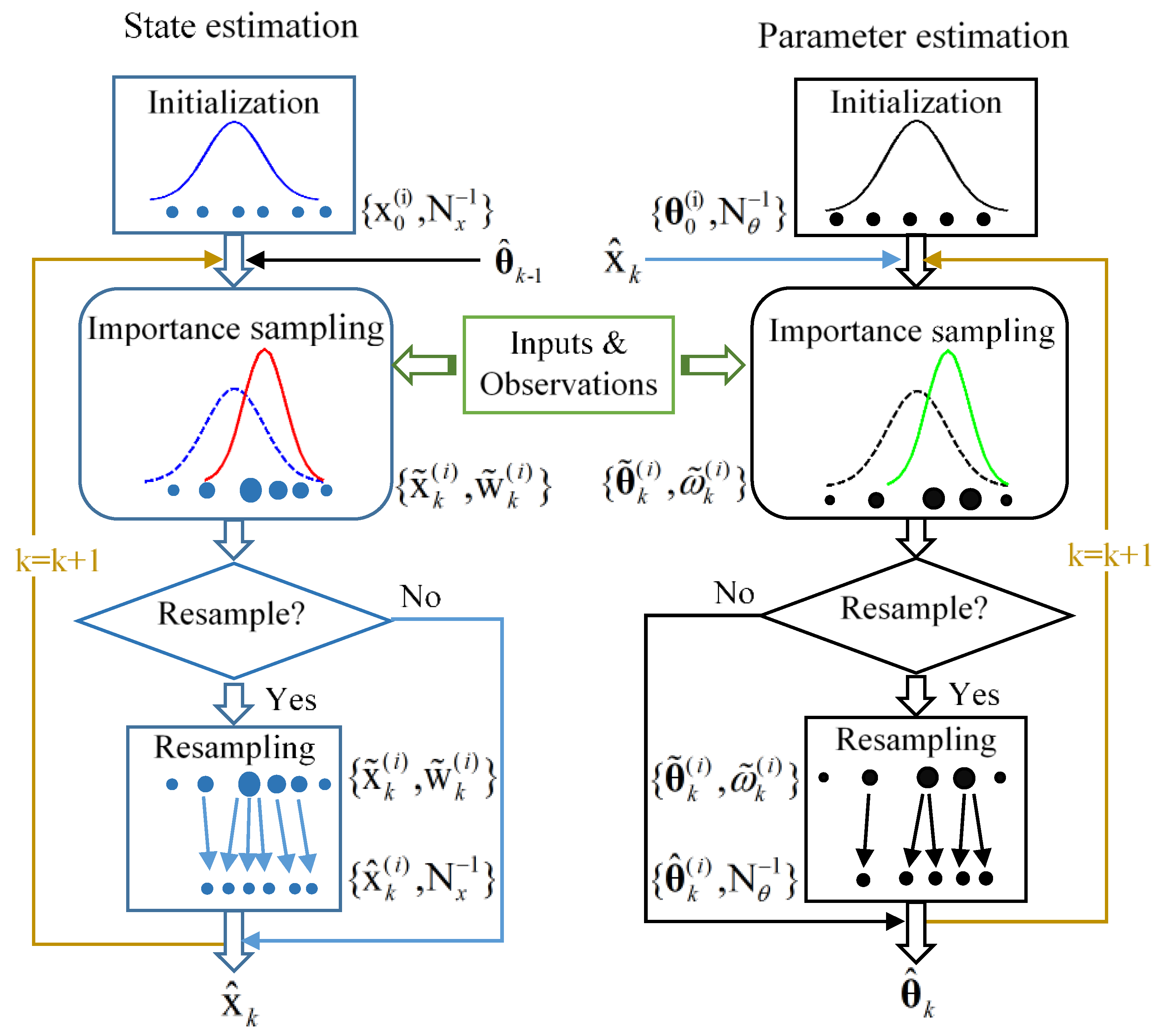
3.3. Dual Estimation

PF provides us a joint estimation of the model parameters and states. However, the standard PF is unstable and inaccurate for estimating high-dimension states and nonlinear coupled states. In the case of RUL prediction, the state is coupled with the parameters, and the clean state is unavailable due to the measurement noise. Thus, a dual-estimation framework [37,38,39] is employed here for model identification.

In our study, two PFs run concurrently given the noisy observations and the condition of rest time. At each cycle k, the PF state filter estimates the state $C_k$ using the previously estimated parameters $\{{\widehat{\alpha }}_{k-1},{\widehat{\beta }}_{k-1}\}$, because the parameters of the kth cycle are not estimated yet. The PF parameter filter estimates the parameters by incorporating the latest estimated state ${\widehat{C}}_k$. Algorithm 1 describes the dual-particle filter algorithm, and Figure 2 shows the dual-PF estimator system schematically.

Algorithm 1: Dual-particle filter algorithm.

1.   Initialization, $k=0$. Generate $N_x$ initial particles ($i=1,\dots ,N_x$) of capacity $x_0^{\left(i\right)}$ from the prior $p\left(x_0\right)$, $w_0^{\left(i\right)}=N_x^{-1}$; $\theta ={[\alpha ,\beta ]}^T$, $N_{\theta }$ initial particles ($i=1,\dots ,N_{\theta }$) of capacity ${\theta }_0^{\left(i\right)}$ from the prior $p\left({\theta }_0\right)$, ${\omega }_0^{\left(i\right)}=N_{\theta }^{-1}$. 2.   For $k=1,2,3,\dots$ (1)   State estimation (a)   Importance sampling. For $i=1,\dots ,N_x$ •   Sample: ${\widehat{x}}_k^{\left(i\right)}\sim q(x_k|x_{0:k-1}^{\left(i\right)},{\widehat{\theta }}_{k-1},y_{1:k})$, and set ${\widehat{x}}_{0:k}^{\left(i\right)}\triangleq (x_{0:k-1}^{\left(i\right)},{\widehat{x}}_k^{\left(i\right)})$ •   Recursively update the importance weights: $$w_k^{\left(i\right)}\propto w_{k-1}^{\left(i\right)}\frac{p(y_k|{\widehat{x}}_k^{\left(i\right)},\widehat{{\theta }_{k-1}})p({\widehat{x}}_{k-1}^{\left(i\right)}|{\widehat{x}}_{k-1}^{\left(i\right)}),{\widehat{\theta }}_{k-1}}{q({\widehat{x}}_k^{\left(i\right)}|x_{0:k-1}^{\left(i\right)},\widehat{{\theta }_{k-1}},y_{1:k})}.$$ (13) •   The normalized importance weights are: $${\tilde{w}}_k^{\left(i\right)}=w_k^{\left(i\right)}[\sum _{j=1}^N{w}_k^{\left(i\right)}].$$ (14) (b)   Resample the state particles ${\widehat{x}}_{0:k}^{\left(i\right)}$ when the effective sample size $N_{eff}$ is below an empirical threshold $N_T$, and the effective sample size is estimated by ${\widehat{N}}_{eff}=\frac{1}{{\sum }_{i=1}^{N_x}{({\tilde{w}}_k^{\left(i\right)})}^2}$; (c)   The estimated state is: ${\widehat{x}}_k={\sum }_{i=1}^{N_x}{\tilde{w}}_k^{\left(i\right)}{\widehat{x}}_k^{\left(i\right)}$. (2)   Parameter estimation (a)   Importance sampling. For $i=1,\dots ,N_{\theta }$ •   Sample: ${\widehat{\theta }}_k^{\left(i\right)}\sim q({\theta }_k|{\theta }_{0:k-1}^{\left(i\right)},{\widehat{x}}_k,y_{1:k})$, and set ${\widehat{\theta }}_{0:k}^{\left(i\right)}\triangleq ({\theta }_{0:k-1}^{\left(i\right)},{\widehat{\theta }}_k^{\left(i\right)})$ •   The importance weights of the parameters are recursively updated as: $${\omega }_k^{\left(i\right)}\propto {\omega }_{k-1}^{\left(i\right)}\frac{p(y_k|{\widehat{\theta }}_k^{\left(i\right)},{\widehat{x}}_k)p({\widehat{\theta }}_k^{\left(i\right)}|{\widehat{\theta }}_{k-1}^{\left(i\right)}),{\widehat{x}}_k}{q({\widehat{\theta }}_k^{\left(i\right)}|{\theta }_{0:k-1}^{\left(i\right)},{\widehat{x}}_k,y_{1:k})}.$$ (15) •   The normalized importance weights are: $${\tilde{\omega }}_k^{\left(i\right)}={\omega }_k^{\left(i\right)}[\sum _{j=1}^N{\omega }_k^{\left(i\right)}].$$ (16) (b)   Resample the parameter particles ${\widehat{\theta }}_{0:k}^{\left(i\right)}$ with similar rules, and obtain the new particles with equal importance weights. (c)   The parameters are estimated by: ${\widehat{\theta }}_k={\sum }_{i=1}^{N_{\theta }}{\tilde{\omega }}_k^{\left(i\right)}{\widehat{\theta }}_k^{\left(i\right)}$.

3.4. Kernel Smoothing

With the dual-particle filtering framework, we can estimate the state and model parameters, respectively. However, the model parameters and state evolve artificially with random noise, as shown in Equations (10) and (11). The state and parameters cannot be decoupled explicitly so far. In this subsection, we aim to reduce the evolving magnitude of the model parameters compared to the state. The rationale behind this is that we want the state to respond to most of the measurement observations and the control inputs, while the model parameters evolve as smoothly as possible. Kernel smoothing [40,41] was originally proposed to avoid the variance dispersion during the artificial evolution of time-varying states. The kernel smoothing of our model parameters has been adopted to shrink the variance of the model parameters, which reduces the impact of the control inputs and measurement observations on the model parameters. The updating of the model parameters in Equation (10) can be revised as follows.

$$\begin{array}{cc}\hfill m_k^{\left(i\right)}& ={\widehat{\theta }}_{k-1}^{\left(i\right)}+ϵ,ϵ\sim N(0,{\sigma }^2),\hfill \end{array}$$

(17)

$$\begin{array}{cc}\hfill {\widehat{\theta }}_k^{\left(i\right)}& =(I-A)m_k^{\left(i\right)}+A(\frac{1}{N_{\theta }}\sum _1^{N_{\theta }}{m}_k^{\left(i\right)}),\hfill \end{array}$$

(18)

where $\theta ={[\alpha ,\beta ]}^T$ denotes the parameters, $m_k^{\left(i\right)}$ is the intermediate variable of $\theta$ for the ith particle in the updating time step of k, I is identity matrix, and $A=[{\lambda }_1,0;0,{\lambda }_2]$ is a diagonal matrix to shrink the variance among the updated particles. When ${\lambda }_1={\lambda }_2=0$, there is no shrinkage and the updating function is the same as in Equation (10). The meanings of other symbols are the same as the previous notations.

3.5. Remaining Useful Life Prediction

The RUL is the remaining cycles before the health indicator deteriorates to the failure threshold. To fulfill the RUL prediction, we propose a two-phase prognostics framework. The first phase is the model identification as described in previous subsections. The second phase utilizes the identified model for RUL prediction. When we obtain the future predicted capacity via the identified model, we can extrapolate the RUL from Equation (19), as described in our previous study [42].

$$RUL=k_{te}-k_{t0},$$

(19)

where $k_{t0}$ denotes the latest cycle in the model-identification phase in which the observation has been utilized and $k_{te}$ denotes the cycle in which the predicted capacity decreases to the failure threshold for the first time. The overall prognostics framework for the lithium-ion battery is visualized in Figure 3.

The RUL for each state-evolving particle ($RU{L}_i$) can be calculated according to Equation (19), and the posterior pdf for the RUL can be approximated from Equation (20) accordingly.

$$p(RUL|u_{1:k_{t0}},{\tilde{C}}_{1:k_{t0}},u_{(k_{t0}+1):k_{te}})\approx \sum _{i=1}^{N_x}{\tilde{w}}_{k_{te}}^{\left(i\right)}\delta (RUL-RU{L}^i),$$

(20)

where $u_{1:k_{t0}}$ denotes all the operating conditions during the model-identification phase; ${\tilde{C}}_{1:k_{t0}}$ represents all the observations from cycle 1 to cycle $k_{t0}$; $u_{(k_{t0}+1):k_{te}}$ denotes the expected conditions. It should be pointed out that the end cycle $k_{te}$ for each particle may not be the same. The prediction of the RUL thus can be approximated by Equation (21).

$$R\widehat{U}L=\sum _{i=1}^{N_x}{\tilde{w}}_{k_{te}}^{i}RU{L}^i.$$

(21)

4. Experiment Comparisons

4.1. Experiment Settings

In this section, we adopt the accelerated aging battery datasets from the NASA Prognostics Center of Excellence (PCoE) [43] for model identification and RUL prediction. The datasets include the operational parameters and conditions for four lithium-ion batteries (#5, 6, 7, and 18) during the degradation experiments. Each battery has been sequentially run with three different operational profiles (i.e., charge, discharge, and impedance) and repeated until their capacities fade to the failure threshold. To validate the efficiency of our proposed model and the model-identification method, we compared the prediction performance of our proposed framework with Saha’s model [19] over the four lithium-ion battery datasets. We also compared the RUL prediction performance of our proposed empirical model with two different parameter-estimation methods. One is dual-particle filtering plus the kernel smoothing method for estimating the state and parameters separately; the other is the particle filtering method for estimating the augmented state/parameter vector.

In the comparison experiments, the prediction starts from different degradation stages. The historical data before the prediction start points were employed for model identification. To enlarge the prediction length and utilize most of the degradation data, we define the failure thresholds for the #5 and #6 batteries as 70% of the original capacity and 75% of the initial capacity for the #7 and #18 batteries. The difference in the selected failure threshold is due to the different cycle lengths and different initial capacities of the four lithium-ion batteries. However, the choice of the failure threshold should consider the reliability of the battery in practice. The actual life (AL) of the battery is the cycle length in which the battery capacity degrades from its initial value to the failure threshold. We may regard the life cycle in 40%, 60%, and 80% of AL as the early, middle, and later stage of the degradation process, respectively. For each setting of the comparison experiments, the fitting and prediction results may differ due to the probabilistic estimation with the particle filtering framework. To capture the statistical information, we ran each experiment 15 times.

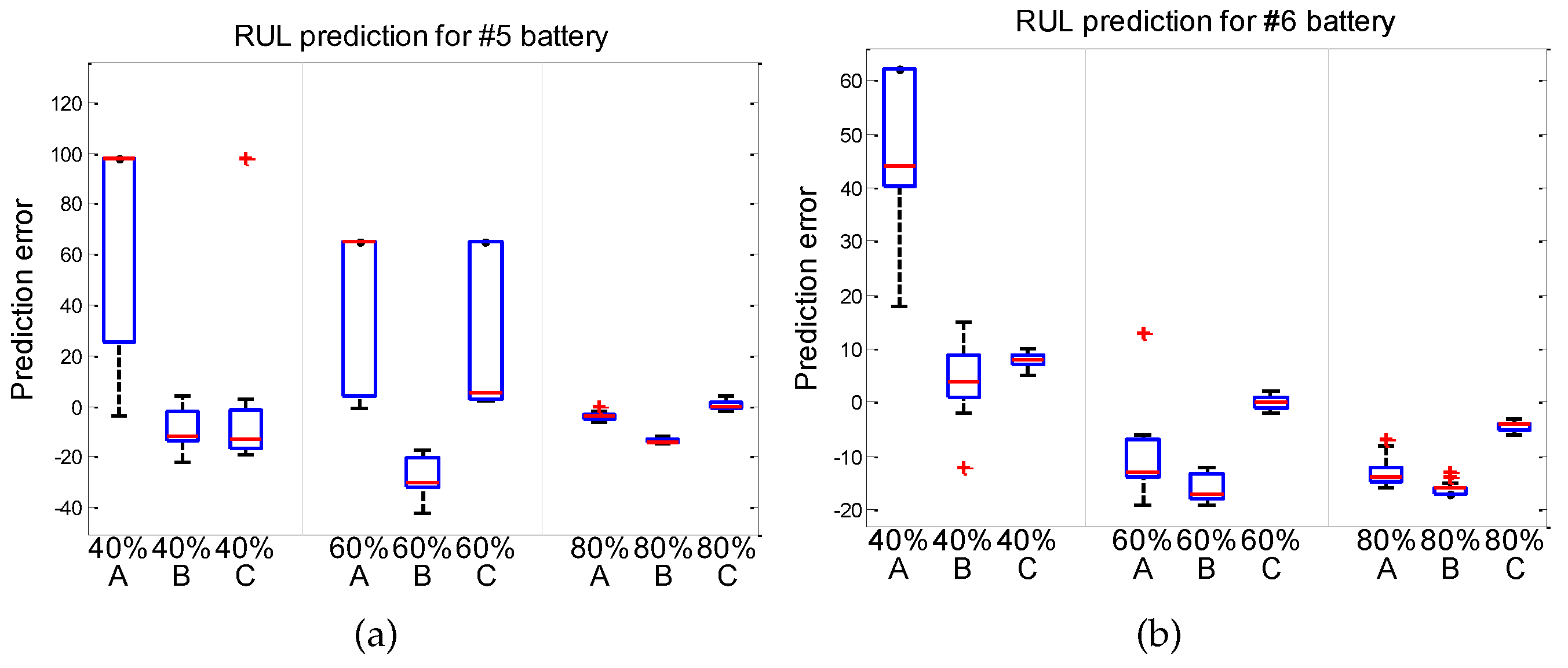
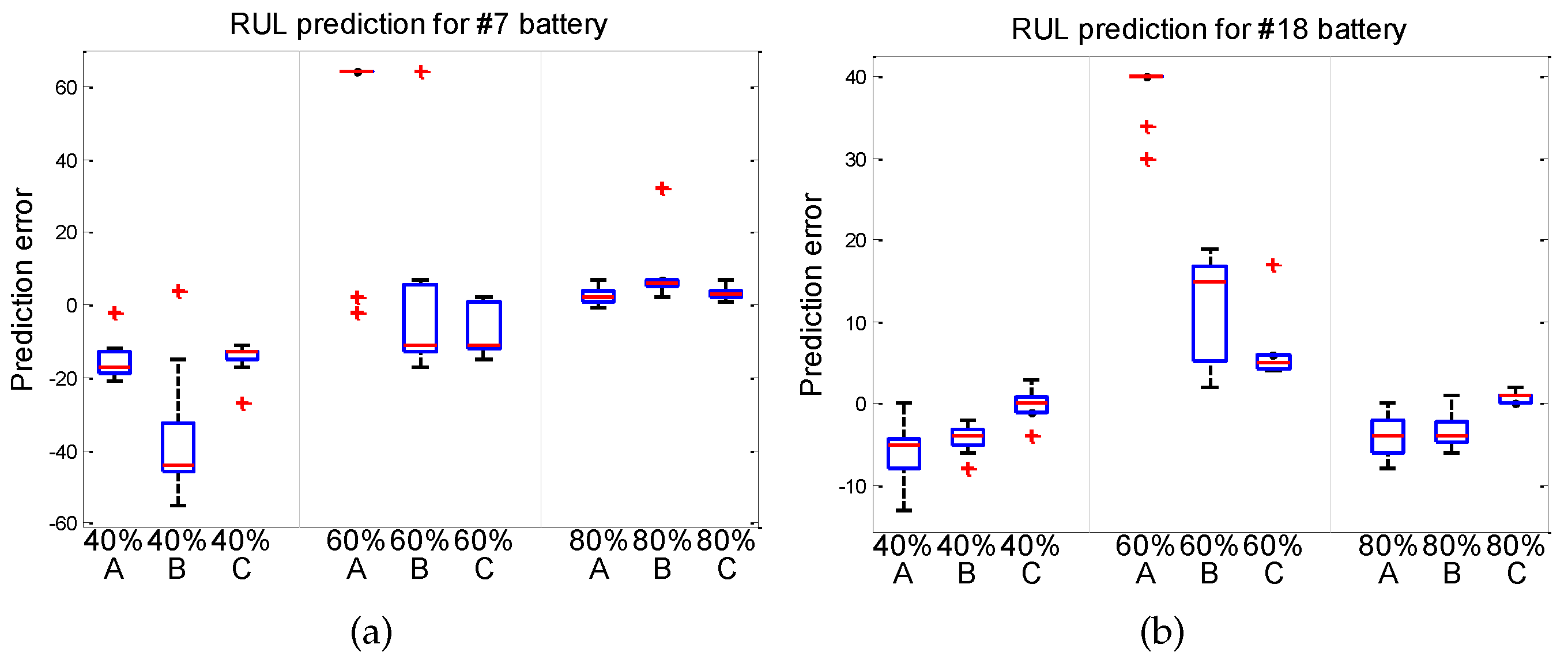
4.2. Results and Discussions

The capacity prediction results for the #5 battery dataset are shown in Figure 4, which visualizes one of the capacity fittings and prediction results among the 15 repeated experiments. The capacity-prediction results for the other battery datasets are similar and not visualized here due to the limited space. Subfigures (a), (b), and (c) of Figure 4 compare the different capacity-prediction performances in different degradation stages, respectively. The methods A, B, and C are used here for simplification to represent Saha’s model (refer to Equation (1)) estimated with particle filtering, our proposed model (refer to Equation (7)) estimated with particle filtering, and our proposed model estimated with dual PF plus the kernel smoothing method (refer to Equations (17) and (18)), respectively. In each subfigure, the vertical dashed line represents the cycle position in which the measurement capacity before the position is fed into the model for model identification; the posterior estimations of these capacities are visualized in the figure before the vertical dashed line. After the dashed line, we use the identified model to predict future capacities. The bold horizontal line represents the failure threshold or end threshold for the battery life. The hollow circle is the measurement capacity on each charge/discharge cycle, and the other lines are the capacity estimations or predictions for different methods. The true RUL is the cycle duration from the dashed line position to the cycle when the bold line intersects with the hollow circle line for the first time, and the predicted RUL can also be visualized in a similar way. From these figures, we can observe that our proposed model and estimation framework are capable of capturing the regeneration phenomenon on the condition of future expected rest time.

Figure 5 and Figure 6 summarize RUL prediction errors for the three modeling methods for different degradation stages. The boxplot groups the results from the 15 repeated experiments. The red line within each box depicts the median of the prediction errors, and the range of the blue box reflects the RUL prediction errors between the 25th percentiles and 75th percentiles. From these figures, we can observe that the prediction errors gradually reduce over the degradation stage, and the prediction errors of our proposed modeling method (method C) are smaller than the other modeling methods regarding both the median errors and repeated variance in general. In the experiments, the prediction line of capacity may not hit the end threshold, leading to the failure of RUL prediction, as shown in Figure 4a. In this case, we penalized the predicted RUL as twice the true RUL for the model comparisons. The quantitative results for all the methods for the four battery datasets are shown in

Table 1. The comparison of RUL prediction performance for different modeling methods.

Battery No.	True RUL	Method A		Method B		Method C
		Median Prediction	Absolute Error	Median Prediction	Absolute Error	Median Prediction	Absolute Error
B0005	98	196	98	86	12	85	13
	65	130	65	35	30	70	5
	33	29	4	19	14	33	0
B0006	62	106	44	66	4	70	8
	41	28	13	24	17	41	0
	21	7	14	5	16	17	4
B0007	96	83	13	52	44	82	14
	64	128	64	68	4	53	11
	32	35	3	36	4	35	3
B0018	60	55	5	56	4	60	0
	40	80	40	55	15	45	5
	20	16	4	16	4	21	1

. In the table, the prediction is the median prediction of all 15 results. For each configuration of the comparison experiments, the smallest prediction errors are emphasized with bold type.

As we can see, the prediction of Saha’s model in the early stage of battery life often leads to the failure of the RUL prediction. A possible reason is that the CE changes for different degradation stages, and the model cannot capture the change of capacity with the fixed CE. In contrast, our proposed model can capture the change of the capacity degradation in most of the cases, which demonstrates that the adaptive modeling method is effective. When we compared the augmented PF estimation method (method B) with our proposed dual PF plus kernel smoothing estimation method (method C), our proposed method is more accurate with less variance in most of the RUL prediction cases. In general, the prediction performance improves when more measurement observations are available in the later degradation stage, and our proposed model and estimation framework (method C) performs better than other modeling methods in most of the cases.

We also compared the parameter-evolving paths for the random evolving in the augmented PF and kernel smoothing evolving in the DPF for our proposed model. As shown in Figure 7, we found that the kernel smoothing-evolving method works well for the updating of the parameters. The evolving paths are smoother, and the changes of the parameters are smaller compared to the randomly evolving method, which demonstrates the effectiveness of our proposed kernel smoothing method.

5. Conclusions

In this paper, a condition-based adaptive model has been developed to model the battery degradation and regeneration process, and a dual-particle filter estimation framework with the kernel smoothing method has been proposed to estimate the model parameters. It has been theoretically proven that the proposed model is equivalent to other state-of-the-art models in capturing the dynamic degradation process, yet with a simpler structure. The rest-time-based regeneration-detection module was proposed and incorporated into the adaptive model. On the condition of the expected rest time, our proposed model allows for multi-step-ahead prediction of the capacity degradation and regeneration. The dual-particle filtering method was utilized to decouple the estimation of the model state and model parameters. The kernel smoothing method was applied to further smooth the evolving path of the parameters, which led to the model state responding to most of the regeneration phenomena during the identification. With the identified model, the future capacity can be predicted based on the condition of the expected rest time, and the RUL can be extracted accordingly. The experimental results demonstrated the satisfactory performance of our proposed method in modeling the degradation and regeneration phenomena. The improvements of our method are both effective in the adaptive model and the dual PF plus kernel smoothing-estimation framework. Our proposed modeling methods are superior in terms of both the RUL prediction accuracy and the repeated variance. However, the real operating conditions of a lithium-ion battery are more complicated than the accelerated aging experiments. For example, the depth of charge or discharge may vary from cycle to cycle in real applications, while the working conditions like temperature or ambient conditions may also affect the degradation and regeneration process. These factors need to be further considered in future work.

References

1. Lu, L.; Han, X.; Li, J.; Hua, J.; Ouyang, M. A review on the key issues for lithium-ion battery management in electric vehicles. J. Power Sources 2013, 226, 272–288. [Google Scholar] [CrossRef]
2. Huggins, R. Advanced Batteries: Materials Science Aspects; Springer Science & Business Media: New York, NY, USA, 2008. [Google Scholar]
3. Liu, K.; Hu, X.; Yang, Z.; Xie, Y.; Feng, S. Lithium-ion battery charging management considering economic costs of electrical energy loss and battery degradation. Energy Convers. Manag. 2019, 195, 167–179. [Google Scholar] [CrossRef]
4. Li, W.; Fan, Y.; Ringbeck, F.; Jöst, D.; Sauer, D.U. Unlocking electrochemical model-based online power prediction for lithium-ion batteries via Gaussian process regression. Appl. Energy 2022, 306, 118114. [Google Scholar] [CrossRef]
5. Xu, J.; Sun, C.; Ni, Y.; Lyu, C.; Wu, C.; Zhang, H.; Yang, Q.; Feng, F. Fast identification of micro-health parameters for retired batteries based on a simplified P2D model by using padé approximation. Batteries 2023, 9, 64. [Google Scholar] [CrossRef]
6. You, G.w.; Park, S.; Oh, D. Real-time state-of-health estimation for electric vehicle batteries: A data-driven approach. Appl. Energy 2016, 176, 92–103. [Google Scholar] [CrossRef]
7. Remmlinger, J.; Buchholz, M.; Meiler, M.; Bernreuter, P.; Dietmayer, K. State-of-health monitoring of lithium-ion batteries in electric vehicles by on-board internal resistance estimation. J. Power Sources 2011, 196, 5357–5363. [Google Scholar] [CrossRef]
8. Eddahech, A.; Briat, O.; Woirgard, E.; Vinassa, J.M. Remaining useful life prediction of lithium batteries in calendar ageing for automotive applications. Microelectron. Reliab. 2012, 52, 2438–2442. [Google Scholar] [CrossRef]
9. Ng, S.S.; Xing, Y.; Tsui, K.L. A naive Bayes model for robust remaining useful life prediction of lithium-ion battery. Appl. Energy 2014, 118, 114–123. [Google Scholar] [CrossRef]
10. Yang, F.; Wang, D.; Xing, Y.; Tsui, K.L. Prognostics of Li(NiMnCo)O2-based lithium-ion batteries using a novel battery degradation model. Microelectron. Reliab. 2017, 70, 70–78. [Google Scholar] [CrossRef]
11. Liu, D.; Pang, J.; Zhou, J.; Peng, Y.; Pecht, M. Prognostics for state of health estimation of lithium-ion batteries based on combination Gaussian process functional regression. Microelectron. Reliab. 2013, 53, 832–839. [Google Scholar] [CrossRef]
12. Ramadass, P.; Haran, B.; Gomadam, P.M.; White, R.; Popov, B.N. Development of first principles capacity fade model for Li-ion cells. J. Electrochem. Soc. 2004, 151, A196–A203. [Google Scholar] [CrossRef]
13. Chen, Z.; Shen, W.; Chen, L.; Wang, S. Adaptive online capacity prediction based on transfer learning for fast charging lithium-ion batteries. Energy 2022, 248, 123537. [Google Scholar] [CrossRef]
14. Liu, K.; Li, Y.; Hu, X.; Lucu, M.; Widanage, W.D. Gaussian Process Regression With Automatic Relevance Determination Kernel for Calendar Aging Prediction of Lithium-Ion Batteries. IEEE Trans. Ind. Inf. 2020, 16, 3767–3777. [Google Scholar] [CrossRef]
15. Chen, Z.; Chen, L.; Ma, Z.; Xu, K.; Zhou, Y.; Shen, W. Joint modeling for early predictions of Li-ion battery cycle life and degradation trajectory. Energy 2023, 277, 127633. [Google Scholar] [CrossRef]
16. Liu, D.; Luo, Y.; Liu, J.; Peng, Y.; Guo, L.; Pecht, M. Lithium-ion battery remaining useful life estimation based on fusion nonlinear degradation AR model and RPF algorithm. Neural Comput. Appl. 2014, 25, 557–572. [Google Scholar] [CrossRef]
17. Xing, Y.; Ma, E.W.; Tsui, K.L.; Pecht, M. An ensemble model for predicting the remaining useful performance of lithium-ion batteries. Microelectron. Reliab. 2013, 53, 811–820. [Google Scholar] [CrossRef]
18. Saha, B.; Goebel, K.; Christophersen, J. Comparison of prognostic algorithms for estimating remaining useful life of batteries. Trans. Inst. Meas. Control. 2009, 31, 293–308. [Google Scholar] [CrossRef]
19. Saha, B.; Goebel, K. Modeling Li-ion battery capacity depletion in a particle filtering framework. In Proceedings of the Annual Conference of the Prognostics and Health Management Society, San Diego, CA, USA, 27 September–1 October 2009; pp. 2909–2924. [Google Scholar]
20. Saha, B.; Goebel, K.; Poll, S.; Christophersen, J. Prognostics methods for battery health monitoring using a Bayesian framework. IEEE Trans. Instrum. Meas. 2009, 58, 291–296. [Google Scholar] [CrossRef]
21. Eddahech, A.; Briat, O.; Vinassa, J.M. Lithium-ion battery performance improvement based on capacity recovery exploitation. Electrochim. Acta 2013, 114, 750–757. [Google Scholar] [CrossRef]
22. Deng, L.; Shen, W.; Wang, H.; Wang, S. A rest-time-based prognostic model for remaining useful life prediction of lithium-ion battery. Neural Comput. Appl. 2021, 33, 2035–2046. [Google Scholar] [CrossRef]
23. Jin, G.; Matthews, D.E.; Zhou, Z. A Bayesian framework for on-line degradation assessment and residual life prediction of secondary batteries inspacecraft. Reliab. Eng. Syst. Saf. 2013, 113, 7–20. [Google Scholar] [CrossRef]
24. Tang, S.; Yu, C.; Wang, X.; Guo, X.; Si, X. Remaining useful life prediction of lithium-ion batteries based on the wiener process with measurement error. Energies 2014, 7, 520–547. [Google Scholar] [CrossRef]
25. Olivares, B.E.; Munoz, M.A.C.; Orchard, M.E.; Silva, J.F. Particle-filtering-based prognosis framework for energy storage devices with a statistical characterization of state-of-health regeneration phenomena. IEEE Trans. Instrum. Meas. 2013, 62, 364–376. [Google Scholar] [CrossRef]
26. Orchard, M.E.; Lacalle, M.S.; Olivares, B.E.; Silva, J.F.; Palma-Behnke, R.; Estévez, P.A.; Severino, B.; Calderon-Muñoz, W.; Cortés-Carmona, M. Information-theoretic measures and sequential monte carlo methods for detection of regeneration phenomena in the degradation of lithium-ion battery cells. IEEE Trans. Reliab. 2015, 64, 701–709. [Google Scholar] [CrossRef]
27. Qin, T.; Zeng, S.; Guo, J.; Skaf, Z. A Rest Time-Based Prognostic Framework for State of Health Estimation of Lithium-Ion Batteries with Regeneration Phenomena. Energies 2016, 9, 896. [Google Scholar] [CrossRef]
28. Pang, X.; Huang, R.; Wen, J.; Shi, Y.; Jia, J.; Zeng, J. A lithium-ion battery RUL prediction method considering the capacity regeneration phenomenon. Energies 2019, 12, 2247. [Google Scholar] [CrossRef]
29. Ma, Q.; Zheng, Y.; Yang, W.; Zhang, Y.; Zhang, H. Remaining useful life prediction of lithium battery based on capacity regeneration point detection. Energy 2021, 234, 121233. [Google Scholar] [CrossRef]
30. Zhang, J.; Jiang, Y.; Li, X.; Luo, H.; Yin, S.; Kaynak, O. Remaining useful life prediction of lithium-ion battery with adaptive noise estimation and capacity regeneration detection. IEEE/ASME Trans. Mechatron. 2022, 28, 632–643. [Google Scholar] [CrossRef]
31. Zhao, L.; Wang, Y.; Cheng, J. A hybrid method for remaining useful life estimation of lithium-ion battery with regeneration phenomena. Appl. Sci. 2019, 9, 1890. [Google Scholar] [CrossRef]
32. Yang, F.; Wang, D.; Zhao, Y.; Tsui, K.L.; Bae, S. A study of the relationship between Coulombic efficiency and capacity degradation of commercial lithium-ion batteries. Energy 2018, 145, 486–495. [Google Scholar] [CrossRef]
33. Yang, F.; Song, X.; Dong, G.; Tsui, K.L. A Coulombic efficiency-based model for prognostics and health estimation of lithium-ion batteries. Energy 2019, 171, 1173–1182. [Google Scholar] [CrossRef]
34. Gordon, N.J.; Salmond, D.J.; Smith, A.F. Novel approach to nonlinear/non-Gaussian Bayesian state estimation. IEEE Proc. F Radar Signal Process. 1993, 140, 107–113. [Google Scholar] [CrossRef]
35. Arulampalam, M.S.; Maskell, S.; Gordon, N.; Clapp, T. A tutorial on particle filters for online nonlinear/non-Gaussian Bayesian tracking. IEEE Trans. Signal Process. 2002, 50, 174–188. [Google Scholar] [CrossRef]
36. Van Der Merwe, R.; Doucet, A.; De Freitas, N.; Wan, E.A. The unscented particle filter. In Advances in Neural Information Processing Systems 13: Proceedings of the 2000 Conference; The MIT Press: Cambridge, MA, USA, 2001; pp. 584–590. [Google Scholar]
37. Wan, E.A.; Nelson, A.T. Dual extended Kalman filter methods. In Kalman Filtering and Neural Networks; John Wiley & Sons, Inc.: New York, NY, USA, 2001; pp. 123–173. [Google Scholar]
38. Storvik, G. Particle filters for state-space models with the presence of unknown static parameters. IEEE Trans. Signal Process. 2002, 50, 281–289. [Google Scholar] [CrossRef]
39. Daroogheh, N.; Meskin, N.; Khorasani, K. A Dual Particle Filter-Based Fault Diagnosis Scheme for Nonlinear Systems. IEEE Trans. Control. Syst. Technol. 2017, 26, 1317–1334. [Google Scholar] [CrossRef]
40. West, M. Mixture models, Monte Carlo, Bayesian updating, and dynamic models. Comput. Sci. Stat. 1993, 24, 325–333. [Google Scholar]
41. Liu, J.; West, M. Combined parameter and state estimation in simulation-based filtering. In Sequential Monte Carlo Methods in Practice; Springer: New York, NY, USA, 2001; pp. 197–223. [Google Scholar]
42. Deng, L.M.; Hsu, Y.C.; Li, H.X. An improved model for remaining useful life prediction on capacity degradation and regeneration of lithium-ion battery. In Proceedings of the 9th Annual Conference of the Prognostics and Health Management Society 2017 (PHM 2017), St. Petersburg, FL, USA, 2–5 October 2017. [Google Scholar]
43. Saha, B.; Goebel, K. Battery Data Set. 2007. Available online: https://ti.arc.nasa.gov/tech/dash/pcoe/prognostic-data-repository/#battery (accessed on 3 May 2016).
Figure 1. The degradation and regeneration phenomena of a lithium-ion battery. For example, the red arrow from bottom to top depicts one of the regeneration phenomena during the battery life cycle, and the blue arrow from left top to right bottom depicts the degradation phenomena.
Energies 17 01679 g001
Figure 2. The dual-particle filter algorithm for state estimation and parameter estimation. The left part is the state estimation, and the right part is the parameter estimation. Both of the estimations iteratively incorporate the newly estimated states or parameters from each other. For example, in the kth step, we estimate the states x ^ k with θ ^ k 1 and, then, estimate the parameters θ ^ k with x ^ k .
Energies 17 01679 g002
Figure 3. The framework of remaining useful life prediction for lithium-ion batteries. The left part is the model-identification phase, which utilizes the dual-particle filtering method and kernel smoothing method; The right part is the RUL prediction phase in which the capacity is continuously predicted with the identified model over the repeated cycle until the predicted capacity hits the failure threshold C T , and the RUL is the cycle duration.
Energies 17 01679 g003
Figure 4. The comparison results for the three modeling methods on the dataset of the #5 lithium-ion battery. Subfigures (ac) show the capacity fitting and prediction results for different degradation stages. The experiments have been repeated 15 times, but Subfigures (ac) only show the results from one of the experiments.
Energies 17 01679 g004
Figure 5. The boxplot of the RUL prediction error by method A, method B, and method C for the #5 and #6 batteries. Method A is Saha’s model estimated with PF; method B is the proposed model estimated with PF; method C is the proposed model estimated with dual PF plus kernel smoothing.
Energies 17 01679 g005
Figure 6. The boxplot of the RUL prediction error for the #7 and #18 batteries. The experiment has been conducted for different degradation stages (40%, 60%, and 80%) of the lithium-Ion batteries; each experiment has been repeated 15 times, and the boxplot summarizes the repeated RUL prediction error.
Energies 17 01679 g006
Figure 7. The comparison of parameter-evolving paths for different evolving methods. The subfigures of (ac) show the parameter-evolving paths for both α and β for different degradation stages. All the subfigures demonstrate that the kernel smoothing method obtains a smoother evolving path than the random evolving method.
Energies 17 01679 g007