Abstract
Global environmental impacts such as climate change require behavior from society that aims to minimize greenhouse gas emissions. This includes the substitution of fossil fuels with other energy sources. An important aspect of efficient and sustainable management of the electricity supply in Brazil is the prediction of some variables of the national electric system (NES), such as the price of differences settlement (PLD) and wind speed for wind energy. In this context, the present study investigated two distinct forecasting approaches. The first involved the combination of deep artificial neural network techniques, long short-term memory (LSTM), and multilayer perceptron (MLP), optimized through the canonical genetic algorithm (GA). The second approach focused on machine committees including MLP, decision tree, linear regression, and support vector machine (SVM) in one committee, and MLP, LSTM, SVM, and autoregressive integrated moving average (ARIMA) in another. The results indicate that the hybrid AG + LSTM algorithm demonstrated the best performance for PLD, with a mean squared error (MSE) of 4.68. For wind speed, there is a MSE of 1.26. These solutions aim to contribute to the Brazilian electricity market’s decision making.
1. Introduction
Electricity plays a fundamental role in the economic and social advancement of nations. Brazil has gained worldwide recognition for its renewable energy mix, with a significant contribution from hydroelectric power. Solar and wind energy also contribute to their renewable energy sources. However, inadequate management and insufficient use of sustainable energy sources can have significant consequences for the country. One critical aspect of energy management is the price of differences settlement (PLD), which reflects the supply and demand of energy in the Brazilian market. Inefficient PLD management can lead to price fluctuations and instability in the supply of electricity. This directly impacts the end consumer, resulting in them facing higher tariffs and lower service quality [1].
Furthermore, excessive reliance in relation to energy sources that are not renewable, such as fossil fuels has significant environmental consequences. Energy generation from these sources contributes to greenhouse gas emissions and climate change, resulting in impacts such as increasing mean temperatures, severe weather occurrences, and elevated sea levels [2,3].
Wind energy, conversely, it is a sustainable option that can have a pivotal impact on diversifying Brazil’s energy matrix [4]. However, the inefficient utilization of wind energy results in missed opportunities to diminish dependence on fossil fuels, alleviate greenhouse gas emissions, and advocate for sustainable development.
The absence of proper electricity management and the underutilization of sustainable energy sources have direct consequences for both the economy and the environment. Rising energy tariffs affect the competitiveness of businesses and the purchasing power of the population. Additionally, environmental degradation caused by the intensive use of fossil fuels threatens ecosystems, biodiversity, and the quality of life.
Therefore, it is crucial to adopt an efficient energy management approach and promote the use of sustainable energy sources like wind energy to ensure a stable, affordable, and environmentally responsible supply of electricity. This requires investments in infrastructure, proper incentives and incentive policies, as well as awareness of the importance of transitioning to a low-carbon economy. Only in this way can we address the energy and environmental challenges, ensuring a sustainable future for future generations.
According to [5], the representation of Brazil’s internal electricity supply originates from the following sources (see Figure 1):
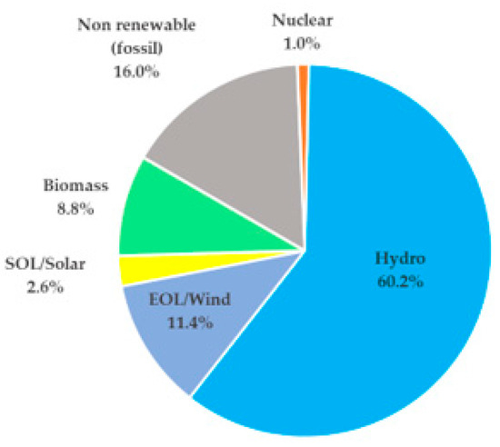
Figure 1.
Electricity production matrix in Brazil.
As observed, hydroelectric generation constitutes the primary source of electrical energy in Brazil. However, contributions from other sources are significant, especially during periods of low rainfall when energy consumption is high.
Currently, the country’s energy matrix incorporates various sources of electrical energy, including hydroelectric and thermoelectric power. Wind energy stands out as one of the most promising forms of generation, particularly in the northeast region which hosts 258 wind farms in Bahia, 225 in Rio Grande do Norte, 105 in Piauí, and 98 in the state of Ceará [6].
On this occasion, the Electricity Trading Chamber (CCEE) of Brazil plays the role of the institution responsible for managing the nation’s electricity market, employing mathematical models to calculate the PLD. This calculation is a crucial metric that guides the value of energy in the short-term market (Mercado de Curto Prazo/MCP). It is important to highlight that several factors are taken into consideration to determine the final PLD value, including the production volume of hydroelectric plants, climatic conditions, fuel prices, deficit costs, energy demand from consumers, and others.
Various computational models are employed for the calculation of the PLD. One example is the NEWAVE, which forecasts energy costs based on the water level in reservoirs for a five-year period. Another model is the DECOMP, which estimates forecast values on average for a horizon of two months.
The CCEE employs the DESSEM model for estimating the PLD, which spans a seven-day interval and aims to optimize the use of thermal generation, enabling a more efficient operation throughout the day. Since January 2021, the CCEE has adopted an hourly PLD, starting to disclose values hour by hour for the next 24 h. This practice ensures greater accuracy and transparency in the short-term formation of electricity prices [1,5,7].
The use of advanced approaches in the management and forecasting of electricity parameters has become increasingly relevant to ensure efficient, sustainable, and reliable supply. In this context, machine committees and the integration of artificial neural networks (ANNs) with genetic algorithms (GAs) have emerged as promising solutions to enhance decision making and optimize resource utilization [8,9].
Machine committees are an approach that combines individual forecasts from different machine learning models, aiming to leverage the diversity of perspectives and specialties [10]. This combination of forecasts allows for more accurate and reliable estimates, reducing the uncertainty associated with electricity parameters.
Furthermore, the integration of ANNs and GAs provides a powerful strategy for tuning the hyperparameters of ANNs, enhancing their learning and data adaptation capabilities [11]. Genetic algorithms, inspired by the biological evolution process, enable the discovery of the ideal parameter combination to optimize the performance of ANNs in predicting electrical parameters.
In this article, we will present a comparative analysis between the machine committee and the combination of ANNs and GAs in the prediction of electrical parameters, focusing on the PLD and wind speed for wind energy. To achieve the objectives of this study, we considered the following approaches and methods: decision tree model, linear regression, auto-regressive integrated moving average and support vector machine, random search, and Bayesian search methods to optimize the hyperparameters of SVM and the auto-ARIMA function with the grid search algorithm to optimize ARIMA parameters. Regarding the approaches involving artificial neural networks, we included long short-term memory and multilayer perceptron with hyperparameters optimized through genetic algorithms. It is important to note that the application of these various classes of models in the same comparative study, aimed at predicting the price of electricity and wind speed in Brazil, is not found in the existing literature. Although there are studies that use forecasting models on the analyzed data, this work significantly contributes to the research field, opening space for future discussions and applications.
The remainder of this research is structured in the following manner: in Section 2, a literature review and an overview of the main related research that fits within the problem’s context will be introduced. In Section 3, the materials and methods used in this research will be outlined. In Section 4, the results of the validation and comparison of predictive models will be presented. Section 5 will conclude with the final considerations.
2. Related Study and Contributions
This section aims to provide an overview of the main research studies addressing the issue of time series prediction in the electric energy sector, with a focus on the Brazilian market. The research started in March 2019 with the support of the Periodicals Portal from the Coordination for the Improvement of Higher Education Personnel (Coordenação de Aperfeiçoamento de Pessoal de Nível Superior/CAPES) [12], which is Brazil’s largest digital scientific collection with access to leading publishers and engineering materials such as IEEE, Elsevier, ACM, Wiley, Emerald, Scopus, and Taylor and Francis. Bibliographic research was conducted using the terms in the first column of Table 1, and the numerical results of the search are represented in the second column of the table.

Table 1.
Results of the bibliographic research.
Energy strategies are of interest to regulatory agencies, local governments, and the business sector. However, reconciling the interests of all stakeholders is not a straightforward task [13], as ensuring effective management requires simultaneous success in various aspects such as energy supply, attracting investments, government fiscal balance, and maintaining affordable tariffs. Furthermore, the current investment in renewable energy indicates a reduction in the consumption of fossil fuels in the future, which has a positive impact on society [14,15].
The ability to anticipate energy demand plays a fundamental role in resource conservation and the prevention of unusual fluctuations in energy consumption [16,17]. In the context of Brazil, the cost of electricity can be considered an optimization challenge that involves evaluating the levels of large hydroelectric reservoirs. When reservoir levels are low, there is a risk of future water scarcity, which necessitates a forecasting analysis for proper assessment [18].
When it comes to electricity price forecasting, Earlier research has highlighted the utilization of machine learning methods, with a notable prevalence of deep learning for predictions [19]. An example of this is the work by Ozcanli [20], which addressed methods and applications of deep learning for electric power systems in a systematic review. Similarly, Abedinia [21] noted a trend in the international literature of combining models with the aim of achieving more accurate forecasts. One of these strategies involves short-term load and electricity pricing forecasting in isolated electricity or energy, using an approach that combines neural networks and a gravity-based optimization algorithm [22].
In line with previous research, Chen [23] addressed the combination of genetic algorithms and models based on machine learning in assessing vulnerability or proneness to landslides. Luo [24] presented a neural network architecture utilizing a genetic algorithm to establish a deep feedforward structure for the daily electricity consumption for the next day and week in a real-world campus building in the United Kingdom. Alencar [25] suggested a combined model integrating time series and neural networks networks for the generation of wind power forecasting. Additionally, the deep learning methodology, based on LSTM recurrent neural networks, combined with the canonical genetic algorithm as mentioned by Junior [26], was applied to assist in the analysis of signals derived from electroencephalogram (EEG) examinations. However, it is crucial to note that, so far, this methodology has not been explored for electricity prediction within the Brazilian context. I would also emphasize that the application of genetic algorithms differs in how the individual/solution is constructed and interpreted, as well as in the procedure applied to the fitness function.
Regarding the use of the genetic algorithm (GA) in combination with MLP and LSTM artificial neural networks for the task of forecasting in the electricity sector, the literature shows that the GA can be used to adjust the hyperparameters of these two neural models or it can be used to find the weights and bias values of both models. In [27], the GA is used to optimize the learning rate and the number of iterations of an LSTM in the task of predicting the short-term load with the LSTM-AG, increasing the prediction accuracy by 63% when compared to the prediction of a standard LSTM. The authors do not state which database is used. Still on load forecasting, Ref. [28] uses the GA to adjust the hyperparameters size of batches, quantity of neurons, activation function, and the epoch duration an LSTM with a feature extractor that defines the inputs of the neural network. The LSTM-AG-extractor has a MAPE error measure of 0.6710, which is lower than that of the LSTM-GA models, LSTM-NSGA-II, LSTM-PSO, and LSTM. In this article, the New England database is used. Ref. [29] uses GA to find the best hyperparameters, the number of window sizes, and the number of units (neurons) of an LSTM to predict short-term solar irradiance. The database used is the the global horizontal irradiance (GHI) at the location of Fes (33.3° N, −5.0° E, Altitude = 579 m), separated by stations. The results of the LSTM-GA prediction model are compared with the LSTM, gate recurrent unit (GRU), and RNN models and the GRU + GA and RNN + AG versions. The findings indicate that the models augmented utilizing GA outperform their respective standard methodologies. In article [30], the authors employ Applying genetic algorithms to optimize the size of the time window for the task. time series, utilized as input data for the RNN. They also optimize the quantity of LSTM units units in the layers in the hidden section and the size of the batches to predict the load of the Australian electrical system, with data collected provided by the operator of the Australian energy market. The outcomes of the simulation emphasize that the recommended hybrid strategy involving GA and LSTM network model exhibits superior performance compared to other conventional models, such as MLP SVM and the traditional LSTM model, yielding the lowest RMSE and MAE values of 87.304 and 118.007, respectively. The suggested model demonstrates an error reduction of 5.89% and 8.19% in comparison to the LSTM approach in RMSE and MAE values. Ref. [31] employs GA to select the optimization algorithm (e.g., Adam, Rmsprop and Sgdm), an initial learning rate δ, and the quantity of hidden layers, as well as the quantity of neurons within each hidden layer of an LSTM to predict wind speed in a city in China (wind energy facilities situated in Inner Mongolia) and in another city in Spain (wind energy installations situated in Sotavento, Galicia). A LSTM + AG ensemble is also utilized to enhance the forecast. The proposed LSTM + AG achieves outperformed the remaining five forecasting models compared (WNN—wavelet neural network, BPNN—backpropagation neural networks, DBN—deep belief network, ELM—extreme learning machine, and standard LSTM), with the best MAE value of 0.53989, RMSE of 0.74116, and MAPE of 8.49605. The standard LSTM was the second-best model, and BPNN was identified as the least efficient model. In [32], researchers employ the GA to fine-tune the dimensions of the time series window and the quantity of neurons in LSTM layers, striving to forecast wind velocity at seven wind farms in Europe. The LSTM + GA model, on average, enhances wind energy forecasts by 6% to 30% compared to existing techniques, such as polynomial kernel SVR, RBF kernel SVR, linear kernel SVR, and standard LSTM. In the study [33], an approach is presented that employs a MLP optimized by a GA to estimate the load of the Australian electrical system. The GA adjusts the number of layers and neurons in the MLP. The optimized model by GA has a hidden layer with ten neurons (given that the MLP has six input variables), achieving a prediction with a Mean Squared Error (MSE) of 4.226 × 10⁻⁷. In the paper [34], a GA is employed to configure the parameters of the MLP, including the activation function, weight and bias adjustment algorithm, and the quantity of neurons in the hidden layer, with the goal for forecasting energy consumption for smart meters. The implemented system initially performs a linear prediction of consumption, followed by a nonlinear prediction of the residual from this linear prediction. Finally, an MLP combines both predictions. The suggested hybrid framework is assessed in comparison when compared to prior methodologies, encompassing individual, ensemble, and hybrid methods. Among the individual models, notable ones include SARIMA (seasonal auto-regressive integrated moving average), MLP, SVR, LSTM, LR (linear regression), and classification and regression trees). The presented results reveal that hybrid models, including the one proposed in the article, outperformed in energy consumption datasets throughout every day of the week. These outcomes were succeeded by ensemble techniques (like bagging) and individual models. The proposed hybrid system was evaluated using information gathered through the smart grid infrastructure implemented in a residential structure. This three-story building is situated in the Xindian district of New Taipei City, Taiwan. It is noteworthy that the referenced studies exclusively focus on one type of data (load/energy consumption, solar irradiance, or wind speed), with none of them utilizing data from Brazil. In [31,35], the same type of data (wind speed) is employed, albeit originating from different databases.
When addressing the use of ensembles, article [32] introduces a the velocity of the wind prediction approach founded on utilizing empirical mode decomposition (EMD) in conjunction with the genetic algorithm-backpropagation neural network (GA-BPNN). The GA is employed to calculate the initial weight values of the BPNN. The collective empirical mode decomposition (EEMD) represents an evolution of EMD, demonstrating effectiveness in resolving the issue of mode blending problem by decomposing transforming the original data into signals with varying frequencies that are more stationary. Every derived signal atcs as input for the GA-BPNN model. The ultimate wind velocity information prediction is derived by combining the individual forecasts from each signal. An examination carried out in a wind facility in Inner Mongolia, China, underscores that the suggested hybrid approach significantly outperforms the traditional GA-BPNN prediction approach, using EMD in conjunction with the Wavelet Neural Network method with EMD and wavelet neural network method in terms of accuracy. A model named ISt-LSTM-informer, employing an enhanced ensemble algorithm called stacking, is proposed in [36] for predicting photovoltaic (PV) energy production. Utilizing a historical data from the DKA solar center, a publicly accessible platform for photovoltaic (PV) power systems in Uluru, Australia, the model employs utilizing the multiple linear regression (LR) algorithm as a meta-model to incorporate meta-features, providing precise near-term and intermediate-term forecasts for photovoltaic power (PVPF). When compared to four other methods (standard LSTM and informer, bidirectional LSTM, BiLSTM, and Autoformer), the ISt-LSTM-Informer showcases superior efficiency throughout all four performance metrics: MAE, MAPE, RMSE and R2. Furthermore, it outperforms a short-term PVPF forecasting model (Stack-ETR) that utilizes a stacking ensemble algorithm with an adaptive boost (AdaBoost), random forest regressor (RFR), and extreme gradient boosting (XGBoost) the foundational models, employing extra trees regressor (ETR) as the meta-model to combination the predictions of the foundational models. In [37], the authors propose a prediction method that combines various models using complementary genetic algorithm-long short-term memory (GA-LSTM), ensemble empirical mode decomposition (CEEMD), particle swarm optimization-support vector machine (PSO-SVM) and radial basis fusion-autoencoder (RBF-AE). This method is employed for load forecasting in the regional integrated energy system (RIES). The load sequence is broken down into frequency intrinsic mode functions (IMF) components using CEEMD. The components of the IMF are categorized according to their zero-crossing points rate and sample entropy (SE), leading to the formation of three distinct categories: high-, medium-, and low-frequency components. Following this, the high-frequency load component, characterized by pronounced randomness, is forecasted through the use of GA-LSTM The load component with medium frequency, characterized by reduced randomness, is forecasted through the utilization of RBF-AE. The steady and cyclical low-frequency load component is forecasted using PSO-SVM The outcomes predicted by these three models are amalgamated to derive the ultimate forecasted value. These results are then compared with the standard BPNN, SVM, RBF, and LSTM models. The multivariate load dataset employed in this study were gathered at the Arizona State University’s Tempe campus in the United States (http://cm.asu.edu/, accessed on 5 January 2024), while the climatic data were acquired from the National Renewable Energy Laboratory (http://maps.nrel.gov/nsrdb-viewer/, accessed on 5 January 2024). The findings validate the effectiveness of the predictive model is effective in handling nonstationary sequences of electricity consumption and demonstrates the ultmost precision in forecasting. In [38], a neural network ensemble framework (eNN) is proposed, employing LSTM, SVM, BPNN, and ELM to forecast wind and solar power generation in China. Three algorithms were employed to improve the accuracy of predictions. Initially, the volatile time series of wind and solar power undergo decomposition into smoothed subsequences using variational mode decomposition (VMD) to mitigate undesirable effects caused by volatility. Subsequently, basic models (ELM SVM, LSTM, and BPNN, ), optimized by the Sparrow exploration algorithm with elite opposition-based learning (EOSSA), are utilized for predicting the generation of wind and solar power based on these decomposed subsequences. Ultimately, the forecasted outcomes from eNN are reconstructed by weighing the predictions among the four models. The weight of each model is determined by the least-squares method. All the data utilized in this investigation were obtained sourced from the statistical data provided by the National Bureau of Statistics of China (https://data.stats.gov.cn, accessed on 7 January 2024). The results indicated that the proposed ENN achieved the lowest metrics of RMSE, MAE, MSE, and MAPE for both wind and solar power forecasting, when compared to the EOSSA-LSTM, EOSSA-ELM, EOSSA-SVM EOSSA-BP models, as well as the conventional ELM, SVM, BPNN, and LSTM models. In the study [39], an innovative multi-stage approach is presented for anticipating electricity prices in commercial and residential settings in Brazil for various temporal horizons (one, two, and three months ahead). The proposed methodology combines an initial pre-processing stage, employing the supplementary ensemble empirical mode decomposition (CEEMD) in conjunction with the optimization algorithm inspired by coyote behavior (COA), aiming to define the hyperparameters of CEEMD. This approach addresses nonlinearities in time series data, enhancing the model’s performance. Subsequently, four machine learning models, namely ELM, Gaussian process, GBM, and the machine of relevant vectors, are applied to train and make predictions the components of CEEMD. Ultimately, in the concluding phase, the outcomes obtained from the preceding stages consist of integrated directly for the formation of a diverse ensemble learning comprising components, with the goal of providing the final forecasts. This data was retrieved from the Institute of Applied Economic Research (IPEA) website accessible at http://www.ipeadata.gov.br/Default.aspx, accessed on 9 January 2024. Through developed comparisons (with standard ELM, Gaussian process, GBM, and RVM, and with homogeneous across multiple stages ensemble models COACEEMD-GBM, COA-CEEMD-GP, COA-CEEMD-RVM, and COA-CEEMD-ELM ), findings indicated that the amalgamation of COA-CEEMD with a diverse ensemble learning approach can generate precise forecasts. These articles work with only one type of data (price, load, solar energy, or wind speed), except in [40] where wind speed and solar energy data are used together. Only [39] used Brazilian data (commercial and residential electricity prices).
The contributions of this article are: (1) to use the GA to adjust the hyperparameters of MLP and LSTM (a hybrid system that is more complex than the MLP and LSTM models, but simpler than an ensemble) to forecast different types of data (prices and wind speed); (2) to compare the results of the AG+MLP and AG + LSTM hybrid systems with heterogeneous ensembles; and (3) to apply these models to Brazilian electricity system.
In this regard, the present the research advocates a methodology that combines the genetic algorithm (GA) with artificial neural networks, particularly long short-term memory (LSTM) networks, that belongs to a distinctive category of recurrent networks, and multi-layer perceptron (MLP) networks to improve predictive accuracy of electricity prices and wind speed in the Brazilian electricity sector. Additionally, it employs a machine committee (ensemble) to aggregate individual model predictions, resulting in improved performance compared to individual models.
3. Methods
In this section, we will discuss the proposed methods and relevant aspects of time series forecasting in the Brazilian market. Two main methods were explored: the ensemble and the combination of deep learning with the genetic algorithm.
In a concise manner, Figure 2 visually represents what is aimed to be modeled and produced through the present study.
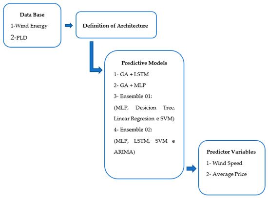
Figure 2.
General scope.
3.1. Artificial Neural Networks with Hyperparameters Optimized by the Genetic Algorithm
Artificial neural networks (ANNs)have demonstrated a powerful model in the field of artificial intelligence and are capable of learning and generalizing from data. However, the effectiveness of ANNs is directly related to the proper configuration of their hyperparameters, which encompass the parameters governing the behavior an functioning of the network [40,41].
To optimize these hyperparameters, the GA is an efficient and robust approach [42]. Derived from the mechanism of biological evolution, the GA uses concepts like natural selection, crossover, and mutation to search for the best combination of hyperparameters for the desired performance of the ANN [43], as illustrated in Figure 3.
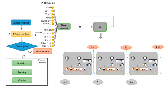
Figure 3.
Predictive time series model combining genetic algorithm and deep learning LSTM (example of electricity price PLD prediction).
The GA operates iteratively, creating an initial population of solutions represented by sets of hyperparameters. These solutions undergo an evaluation process, where they are tested for their performance in a specific task, such as predicting variables in the electricity market. Based on the evaluation, the most promising solutions are selected and crossover to create new solutions. Additionally, some solutions may undergo random mutations to explore new regions of the hyperparameter space. This process is repeated over several generations, allowing the search for progressively better solutions.
The combination of ANN with hyperparameters optimized by the GA offers several advantages [44,45,46]. First and foremost, it allows for finding the ideal configuration of the ANN for the given task, maximizing its performance. Furthermore, this automated approach enables the exploration of a wide range of hyperparameter combinations, finding solutions that may be difficult to identify manually.
3.1.1. Problem Coding
Initially, it is necessary to establish the chromosome, which is the representation or description of the solution or individual that meets the problem’s conditions. This chromosome is composed of variables related to the problem in question, forming a vector of numbers. Everyone is characterized by a sequence of genes with their respective alleles, that is, specific values of the variables that encode the chromosome. The hyperparameters to be optimized by the genetic algorithm encompass the number of layers, the number of cells/neurons, and the definition of dropout in each layer.
In this context, the problem in question can be encoded as shown in Figure 4, which presents the structure of the chromosome and the relationship between the genes and their respective alleles.
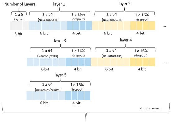
Figure 4.
Integration of genetic algorithm and deep learning LSTM for electricity price prediction (example with PLD).
In Figure 4, individuals are represented genotypically by binary vectors totaling 53 bits. The first group of three genes determines the number of layers in the artificial neural network model—both LSTM and MLP. Then, with each group of 10 bits, the layer structure is defined. The first 6 bits indicate the quantity of neurons/cells within the layer, ranging from 1 to 64, while the remaining 4 bits are used to set the dropout value, which varies from 1 to 16%.
Dropout is a technique that allows for the modification of a neural network by randomly and temporarily deactivating some of the neurons in the intermediate layers. This procedure is like training many different neural networks, which causes the networks to adapt in various ways to address overfitting reduction [47]. This genotypic configuration allows for an efficient representation of the characteristics of the Artificial Neural Networks model, including the quantity of layers and the number of neurons/cells in each layer, and the use of dropout. These variables have a direct impact on the performance and the model’s ability to handle the prediction of PLD and wind speed in wind energy.
3.1.2. Population
In the specific case of this solution, the genetic algorithm is initiated with a predefined number of initial solutions which consists of 80 individuals. Each individual has genes with randomly generated values, providing genetic diversity in the initial population. This randomness is essential for exploring different genetic combinations and seeking optimal solutions for the problem at hand.
3.1.3. Population Assessment
Through the technique of deep learning, the genetic algorithm aims to optimize the parameters of the model for minimize the prediction error. The lower the prediction error, the higher the individual’s fitness within the population, indicating that it is better adapted to the task of predicting PLD and wind speed in wind energy.
3.1.4. Selection
To ensure representativeness and minimize biases that may affect the results, among the various selection strategies, random tournament selection was applied at this stage of the genetic algorithm.
3.1.5. Elitism
The elitist technique was implemented, which involves selecting the “n” best individuals from the previous population to be incorporated into the current population. In this work, n = 1, indicating the top-performing individual from the preceding generation is retained in the current cohort. This ensures that the most promising solution is retained across generations, preventing its loss, and allowing it to be refined over time.
3.1.6. Crossing
In this work, when applying crossing, two cutoff points are arbitrarily designated in the genes of the individuals selected for crossing. These cutoff points divide genes into segments which will be exchanged between parents. The exchange process generates two new individuals, which will make up the new population. The frequency with which the crossover will occur is related to the 75% crossover rate.
3.1.7. Mutation
In the problem at hand, the mutation operator is implemented through a mutation probability check. This probability determines how frequently mutations will occur. For instance, a mutation rate of 1% indicates that, on average, 1% of each individual’s genes will be altered.
3.1.8. Fitness Function Calculation
To use the combination of genetic algorithm with LSTM or MLP, the GA must have access to the fitness information of each individual. Since each individual is a set of hyperparameters that defines a time series predictive model, it is necessary to train the model with these hyperparameters to evaluate its quality.
Therefore, using the genetic algorithm in this combination requires a predictive neural model to be trained quickly to evaluate each set of hyperparameters generated by the GA. This training process is crucial for measuring the quality of each individual and selecting those with higher fitness for solving the problem.
Therefore, the combination of GA + LSTM or GA + MLP requires interaction between the genetic algorithm and the predictive neural model to optimize the search process for the best hyperparameters for the model. It is essential to emphasize that after tuning the hyperparameters of the predictive model, it is imperative to evaluate it to verify its generalization and prediction capability. This step is crucial to ensure that the model can provide accurate and reliable results in real-world situations.
In this process, when evaluating the predictive model, performance metrics are utilized for contrasting the model’s predictions against observed data. To calculate the error of the evaluation function and fitness, mean squared error (MSE) is used.
Long Short-Term Memory
The long short-term memory (LSTM) network is a specialized variation of recurrent neural networks that overcomes the challenge of short-term memory in sequential data. With its input, forget, and output gates, LSTMs can store relevant information for long periods, allowing the modeling of long-term dependencies (see Figure 5). This capability makes LSTMs commonly employed in natural language processing tasks and other applications involving sequence processing [48].
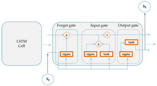
Figure 5.
Scheme of the long short-term memory (LSTM).
The LSTM architecture consists of memory cells that contain a cell state and a gate state. The memory cell is responsible for maintaining long-term memory, while the gates control the flow of information in and out of the cell. The gates are composed of dense layers, each with sigmoid activations ranging between zero and one, allowing the network to decide which information to forget and which to remember [49].
When addressing the structure of the LSTM, our work considered a range of hyperparameters, emphasizing the importance of balancing various elements. Among these hyperparameters, we included the number of memory cells in the LSTM layer. It is crucial to find a balance in this number because excessive increases can boost the network’s capacity but can also slow down training and increase the risk of overfitting.
Another aspect evaluated was the number of LSTM cell layers. Adding layers can enhance the network’s ability to learn more complex representations. We also considered the weight adjustment rate of the network during training, which can expedite the process and help control potential instabilities and divergences.
Additionally, we addressed architecture regularization through techniques like dropout or early stopping. This is crucial to prevent overfitting and ensure proper generalization.
Finally, we considered the batch size and the ReLU activation function. These elements were chosen to speed up training but also to strike a balance between memory requirements and processing power as needed to achieve the specific goals of our study.
Multilayer Perceptron
The multilayer perceptron (MLP) is a versatile neural network architecture consisting of multiple layers of neurons. With its ability to learn complex representations, MLP excels in tasks like classification, regression, and pattern recognition. Training an MLP is accomplished using the backpropagation algorithm, which adjusts the weights of connections between neurons. MLPs are widely applied in various domains, as a result of their capacity to handle nonlinear problems and learn from complex data [50]. MLPs are highly relevant in the machine learning landscape as they form the basis for numerous existing applications (Figure 6) [51].
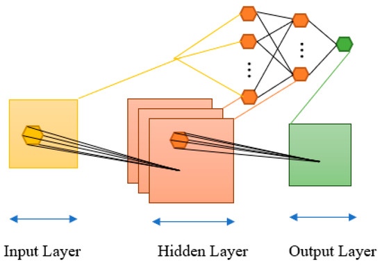
Figure 6.
Multilayer perceptron.
The architecture of MLP consists of multiple layers of neurons, including an input layer, one or more intermediary layers (commonly referred to as hidden layers), and an output layer. Each neuron in a given layer establishes connections with all neurons in the subsequent layer, creating a densely connected network.
Each neuron in an intermediate layer uses an activation function to process the weighted input signals and generate an output.
The training of an MLP involves propagating the training data through the network and adjusting the weights of the connections between neurons to reduce the discrepancy between the network’s predictions and the true labels of the data.
In terms of structuring the MLP, our work considered a set of essential hyperparameters for the same reasons mentioned earlier in relation to LSTM. Among all of the hyperparameters, we included the definition of the quantity of neurons to be assigned in every layerof the network (which directly impacts the model’s representation capacity and complexity) and the quantity of epochs (which specifies how many iterations the network will go through the entire training data set and influence the model’s convergence).
Table 2 summarizes the parameters used for the simulation of the genetic algorithm employed in this work.

Table 2.
Parameters for simulation with GA.
3.2. Ensemble
Ensembles have demonstrated to be a successful method for enhancing the efficiency of machine learning systems [52]. Instead of relying on a single model, a committee consists of multiple learning models (called members) that work together to make more accurate and robust decisions.
The idea behind the ensemble is to exploit the diversity and complementarity of individual models. Each ensemble member can be trained independently using different learning algorithms, datasets, or hyperparameter configurations. By combining the predictions of each member, the committee can capture different perspectives and reduce the impact of individual errors, resulting in more accurate and reliable predictions.
There are several ways to combine the predictions of ensemble members such as voting, boosting, bagging, and other methods. These aggregation techniques allow for the leveraging of leveraging the strengths of each model while alleviating their weaknesses.
Considering the diversity and complementarity of individual models within the ensemble, the strategy adopted to combine the predictions of ensemble members will be the voting method [53]. In this method, each ensemble member predicts a specific sample and calculates the average of their individual predictions to form a final prediction.
Voting is a simple and robust technique that allows you to leverage the different perspectives of ensemble members and mitigate potential individual errors. By relying on the contribution of each model, more accurate and reliable results can be obtained in various learning tasks. We emphasize that the choice of the voting method for this work is based on previous studies and the nature of the problem at hand [54,55,56].
This strategy has proven to be suitable for achieving a balance between accuracy and simplicity in the decision-making process.
The members of the two ensembles will consist of four distinct models: ensemble 01 (decision tree, MLP, linear regression, and SVM) and ensemble 02 (MLP, LSTM, SVM, and ARIMA).It’s crucial to highlight that the establishment of models in ensembles was planned to ensure that each component generalizes in different ways. Additionally, the formation of the models considers the inclusion of those that have shown favorable results in specific applications, as well as indispensable references to monitor the progress in the study. Figure 7 and Figure 8 depict the constituents and the approach for combining votes.
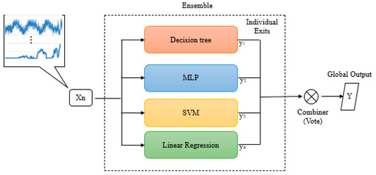
Figure 7.
Machine committee proposal: “ensemble 01”.
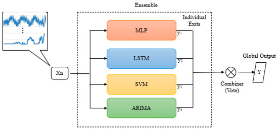
Figure 8.
Machine committee proposal: “ensemble 02”.
This combination of models was selected to explore the diversity of machine learning techniques and their abilities to handle different aspects of the problem at hand [57].
The decision tree is known for its ability to create clear rules and intuitive interpretations, making it useful for making decisions regarding regression assignments and classification.
On the other hand, artificial neural networks are able to deal with more complex problems, leveraging the universal approximation capability of neural networks [58,59].
Linear regression is a traditional technique that provides a simple and interpretable approach to regression problems, while the support vector machine (SVM) is effective at class separation in classification problems [60].
The ARIMA model is a statistical technique used in a variety of scenarios where one wishes to predicting upcoming values by analyzing historical patterns within time series data [61].
By combining these models, we aim to capture different perspectives and characteristics of the dataset, leveraging the individual strengths of each. With this diversity, this combination will provide more accurate and reliable results to achieve the established goals.
The parameters of these prediction models in the ensembles are summarized in Table 3 and Section 3.3.3.

Table 3.
Ensemble member hyperparameters.
3.3. General and Relevant Aspects of the Proposed Models
3.3.1. Database
In this work, two real databases from the Brazilian electricity market were used. The first database was that of the price of differences settlement (PLD) from the Brazilian National System. This database contains records of electricity prices in the northern region, covering the period from 4 August 2001 to 16 December 2009, with 440 weekly samples [62]. Furthermore, we used the wind energy database, which contains information from a location in the northeastern region of Brazil: Macau (latitude 5°9′3.726″ south, longitude 36°34′23.3112″ west). This database covers the period from 1 June 2016 to 31 May 2017, and contains a total of 4900 samples [63].
For the prediction of the PLD, the following variables were used: hydro generation (GH) and thermal generation (GT), energy load (CE), PLD price (P), as well as the levels of reservoirs EARM and ENA. The selection of these variables was performed using the technique of explanatory variable ranking, which assesses the predictive power of each variable individually based on a criterion function [18].
For the measurement of wind speed in wind turbines in the northeast of Brazil, the following variables were considered: wind speed (SW), air temperature (TA), air humidity (HA), atmospheric pressure (PA), and wind direction (DW). The meteorological time series used in this work were obtained from the database provided by the National Organization System for Environmental Data (SONDA). To ensure the quality of the data obtained by the SONDA station, the data quality control strategy used by the Baseline Surface Radiation Network (BSRN) was adopted.
To facilitate the analysis of data behavior and identify patterns or trends, PLD and wind speed data are graphically represented. Figure 9 and Figure 10 illustrate the scatter matrix.
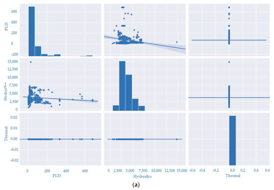
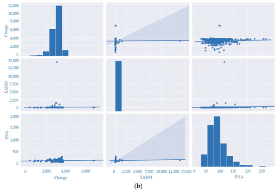
Figure 9.
Scatter matrix plot for six PLD variables in the north region of Brazil. (a) graphical representations of the relationship between three numerical variables (PLD, Hydraulics and Thermal). (b) graphical representations of the relationship between three numerical variables (Charge, EARM and ENA).each point represents the value of one variable on the horizontal axis and the value of another variable on the vertical axis.
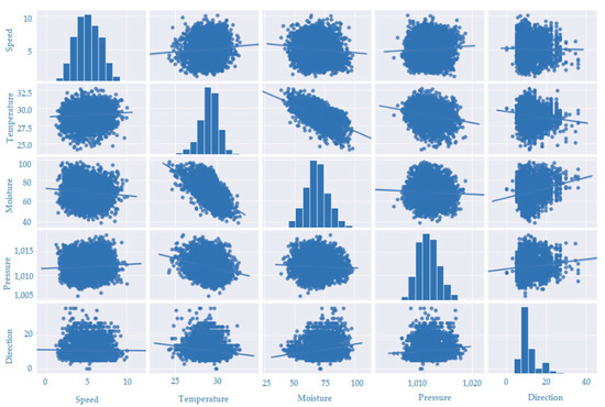
Figure 10.
Scatter matrix plot for five wind speed variables in Macau.
During the occasion, the matrix consists of a series of scatter plots that relate the variables pairwise. Each point in the matrix represents an observation of the respective variables. The diagonal plots consist of individual histograms for each variable, displaying the frequency distribution of the specific data for that variable. This provides a comprehensive view of the data distribution, enabling the identification of potential anomalies or deviations from a normal distribution.
In Figure 10, we observe the scatter matrix for five variables related to wind speed in Macau: speed, temperature, moisture, pressure, and direction. Each variable is plotted on a separate axis, and the points on the graph represent the observed values for each variable.
When analyzing the position of points in the scatter matrix, we can identify potential relationships between variables. For instance, we observe a negative correlation between wind speed and pressure, suggesting that as atmospheric pressure increases, wind speed tends to decrease. Conversely, there appears to be a positive correlation between wind speed and temperature, indicating that as temperature rises, wind speed also tends to increase. Additionally, it is crucial to note that wind direction may also influence wind speed.
Table 4 and Table 5 display the statistical analyses related to the six and five time series, respectively. These analyses include measures of central tendency and dispersion, providing a comprehensive overview of the data.

Table 4.
Position and dispersion measurements in the north region.

Table 5.
Macau position and dispersion measurements.
3.3.2. Preprocessing
The input variables used in the training and testing of the predictor underwent a normalization preprocessing [1]. This process involves scaling the data to the common range of zero to one without distorting the differences in value ranges.
For the deep artificial neural network and genetic algorithm, a holdout sampling method was applied to obtain more reliable estimates of predictive performance by defining a training and testing subset [64]. Each database had its samples divided into 75% for training (used for model induction and adjustments) and 25% for testing (simulating the prediction of new objects to the predictor that were not seen during the training phase).
Figure 11a,b display the time series of PLD data in the north region of Brazil and wind speed data in the city of Macau, respectively. These visualizations allow for the observation of the data’s variation over time. In the graph, the blue color represents the training set, and the red color represents the testing set.

Figure 11.
(a) Division of the dataset into training and testing sets for the PLD—North; (b) division between the training and testing sets for the wind speed database—Macau in the second panel.
To simulate the ensemble members, the data for PLD and wind speed underwent preprocessing (data cleaning, handling missing values, data normalization, encoding categorical variables, etc.). During this preprocessing we used a data balancing technique, which aims to evenly distribute the work or load among available resources [65]. This procedure ensures that the data is balanced and representative for subsequent analysis. After balancing, the data was split into training and evaluation datasets. We chose a proportion of 75% for the dataset for training purposes and 25% for the testing set. This division is of great importance as it allows us to evaluate the model’s effectiveness in an independent test scenario and assess its ability to generalize to new data.
3.3.3. Techniques and Methods to Optimize Parameters
For the creation of ARIMA and SVM members, a different strategy was adopted compared to the one used by the genetic algorithm [66]. Instead of using the genetic algorithm to fine-tune the parameters of these models, random search and Bayesian search methods were employed for SVM, and the auto-ARIMA function from the pm-ARIMA library in Python, along with the grid search algorithm, was used for ARIMA [67]. Table 6 summarizes the hyperparameter optimization.

Table 6.
Application of hyperparameters.
3.3.4. Assessment Metric
To validate the developed models, the statistical performance measure called mean squared error (MSE) was used. This measure provides insights into the model’s behavior with respect to the analyzed data, allowing an assessment of how well it can make accurate predictions. While there are other performance measures available, MSE was considered the most suitable for this study due to its beneficial haracteristics for regression problems as well as information obtained from [68,69].
3.3.5. Training Cost
The entirety of the experiments was conducted on a single computational system equipped with an Intel Core i5 processor, 8 GB of RAM, and 128 GB SSD storage. The choice of the Python programming language was grounded in several criteria, encompassing its prevalence in the field of data science and machine learning, as well as the availability of an extensive array of libraries and specialized tools, simplifying the implementation and analysis of the models.
The average time cost for training the models was approximately two days for individual algorithms, five days for machine ensembles, and nine days for the hybridization between deep learning, enhanced through optimized hyperparameters via the canonical genetic algorithm.
4. Results and Discussion
In this segment, we will showcase the outcomes. obtained from the combination of two machine learning models with the genetic algorithm (GA): GA + LSTM and GA + MLP. Additionally, we will also discuss the performance of the Ensembles.
4.1. Results of the GA + LSTM and GA + MLP Combination
4.1.1. Results of the Combination for PLD
Next, the results of the model development combining GA + LSTM and the combination of GA + MLP are presented for the purpose of comparison. The outcomes can be found in Table 7.

Table 7.
MSE of the GA + deep learning combination.
When evaluating the outcomes of the approach suggested in this study, it can be observed that the model with the combination of GA + LSTM network yielded satisfactory results, achieving better performance for the price of settlement differences. The results of the GA + LSTM model’s evolution are presented in Figure 12. In this figure, the red curve represents the performance of the best individual over generations, while the blue curve represents the average fitness of the population in each generation.
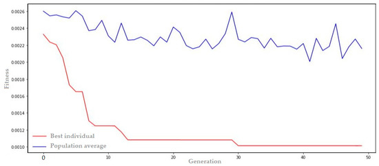
Figure 12.
Optimal settings for GA + LSTM for forecasting the PLD in the north region.
In Figure 12, it is noticeable that the fitness of the best LSTM configuration improves rapidly, indicating a significant reduction in prediction error. Starting from generation 10, the GA begins the convergence process towards an optimal point in the search space for the best LSTM configurations. The key characteristics of the best model can be summarized in the genome transcription below. This transcription represents the best parameters found by the GA for the LSTM configuration:
- Genome transcription: [4, 46, 0.01, 57, 0.0, 2, 0.11, 8, 0.03, 0.00101]
The best solution was obtained through a neural architecture composed of four hidden layers with 46, 57, 2, and 8 cells, respectively. In addition, dropout techniques were applied with rates of 0.01, 0.0, 0.11, and 0.03 in each of these layers. This combination resulted in a prediction error of 0.00101.
4.1.2. Combination Results for Wind Speed
Table 8 presents the outcomes of the experiments carried out for the wind speed dataset.

Table 8.
MSE of the GA + deep learning combination.
For wind speed prediction in the city of Macau, the results indicate that the combination of GA + LSTM outperformed the combination of GA + MLP. Specifically, the GA + LSTM model achieved a slightly lower mean squared error (MSE) compared to the GA + MLP model.
The result of the evolution of the GA + LSTM model for wind speed prediction can be seen in Figure 13.
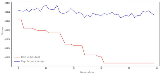
Figure 13.
Optimal settings for GA + LSTM for wind speed prediction.
In Figure 13, it can be observed that the evolution of the best configurations for LSTM shows gradual progress from the early generations. Genetic algorithm convergence begins to occur after approximately generation 30. The key features of the best model, as illustrated in Figure 13, can be summarized in the following genome transcription:
- Genome transcription: [5, 5, 0.03, 45, 0.09, 36, 0.14, 63, 0.04, 2, 0.02, 0.01306]
The best solution was achieved using a neural architecture with five hidden layers. These layers have 5, 45, 36, 63, and 2 cells, respectively. Additionally, the model incorporates a regularization technique known as dropout, with rates of 0.03, 0.09, 0.14, 0.04, and 0.02 applied to each hidden layer. This configuration resulted in a prediction error of 0.01306, indicating good performance of the model in the forecasting task.
4.2. Ensemble Results
In this section, comparative results between “ensemble 01” and “ensemble 02” regarding their effectiveness in forecasting time series, particularly concerning PLD and wind speed parameters, will be presented. Additionally, the outcomes resulting from the replacement of the SVM component as an enhancement strategy will be addressed, highlighting the impact that substituting a model component has on the result.
At this juncture, there are two voting methods: voting average (VOA) and voting weighted average (VOWA). In the case of VOA, the weights are equivalent and equal to one, and the final predicted value is obtained by computing the mean of the predictions generated by individual machine learning models (see Equation (1)):
where m is the number of machine learning algorithms used in the ensemble, represents the value predicted by algorithm j, and is the final predicted value. However, a disadvantage of the VOA method is that all models in the ensemble are considered equally effective, without considering possible performance differences among them.
The VOWA method specifies a weight coefficient for each member of the ensemble. This weight can be a floating-point number between zero and one where the sum of all weights equals one, or it can be an integer number of one, indicating the number of votes assigned to the respective ensemble member. The final predicted value is obtained as shown in Equation (2), where wj represents the weight of algorithm j.
Regarding the results of the ensemble with VOWA, the weight distribution will follow an allocation of integer votes as indicated in Table 9. The model with the highest performance will receive the highest number of votes, while the model with the lowest performance will receive only one vote.

Table 9.
Weights of ensemble model members—VOWA.
The selection of weights as integers and the voting in the VOWA method are justified by their more intuitive interpretation, as they reflect a direct count, facilitating the understanding of results. In addition to the method’s ease of implementation, making it more straightforward and less complex than working with fractional values, it is also easier to track and understand how each group member contributes to the final decision. Expressing the strength of a preference in a discrete form is also more straightforward.
Considering the information provided regarding the voting methods, the results obtained using the VOA and VOWA approaches will be presented.
4.2.1. Ensemble Results for PLD—North Region

Table 10.
Comparative results of members, “ensemble 01” with VOA and “ensemble 01” with VOWA—north region.

Table 11.
Comparative results of members, “ensemble 02” with VOA and “ensemble 02” with VOWA—north region.
In Table 10 and Table 11, you can find the results of the four components individually as well as the results obtained through the combination using the VOA and VOWA voting methods.
The weighted voting, which assigns votes to each model based on its performance, shows an improvement in the results, as evidenced in the table above.
It is notable that in “ensemble 01”, three of the members demonstrated superior capability in approximating the PLD series, while the SVM exhibited the least satisfactory performance.
Both “ensemble 01 and 02” display satisfactory results but fail to surpass the individual performance of the members, except for the SVM.
It is evident that in practice, the main goal is to achieve a performance gain compared to the best available classifier when considered in isolation. However, this improvement may not necessarily result in exceptionally high accuracy rates and may not be able to surpass the performance of individual models due to the “averaging limitation”.
To explain further, the performance of the ensemble is ultimately an average or weighted combination of the predictions from individual models. If one of the individual models, such as SVM, consistently generates “inaccurate or incorrect” predictions, these unfavorable results will eventually negatively impact the overall performance of the ensemble.
To address this issue, the SVM member in “ensemble 01” was replaced with ARIMA. In “ensemble 02”, SVM was replaced with the linear regression model (see Table 12 and Table 13).

Table 12.
Results of “ensemble 01” with the replacement of SVM by ARIMA—north region.

Table 13.
Results of “ensemble 02” with the replacement of SVM by linear regression—north region.
There are numerous other scenarios in which the application of ensembles can prove highly advantageous. However, addressing these diverse scenarios requires a deep understanding of the conditions that must be present to ensure the success of an ensemble approach. Identifying these conditions may sometimes not be a straightforward task, so it is a practical suggestion to apply ensembles and compare the resulting performance with that obtained from individual solutions.
4.2.2. Ensemble Results for Wind Speed—Macau
Here are the errors related to the predictions obtained by the ensemble. Table 14 and Table 15 contain the details of these results.

Table 14.
Comparative results of members, “ensemble 01” with VOA and “ensemble 01” with VOWA—Macau.

Table 15.
Comparative results of members, “ensemble 02” with VOA and “ensemble 02” with VOWA—Macau.
The results of the members indicate satisfactory performance in wind speed prediction.
The inclusion of the SVM model in the final ensemble voting may introduce bias into the results, with VOA showing satisfactory results but not surpassing the demonstrated individual performance.
Below, Table 16 and Table 17 display results with the replacement of the SVM component, namely, in “ensemble 01”, composed of decision trees, MLP, ARIMA, and linear regression, and in “ensemble 02”, composed of MLP, LSTM, linear regression, and ARIMA.

Table 16.
Results of “ensemble 01” with the replacement of SVM by ARIMA—Macau.

Table 17.
Results of “ensemble 02” with the replacement of SVM by Linear Regression—Macau.
Based on the tables above, it is evident that forming the ensemble by replacing the SVM member resulted in more satisfactory predictions, both with VOA and VOWA. Furthermore, the values approached the individual results and, in some cases, outperformed the performance of the ARIMA model.
Figure 12 and Figure 13 compile the best results considering the MSE evaluation metric for one-step-ahead prediction of the models presented in the article. These results are for the PLD datasets from the north region and wind speed in Macau.
On this occasion, the results of the individual members of LSTM and MLP were included in Figure 14 and Figure 15 as part of a baseline with adjusted hyperparameters without the use of the genetic algorithm (parameters defined in Table 3). This baseline integrates the technique of the genetic algorithm to ‘select’ and ‘tune’ the hyperparameters of these algorithms, aiming to enhance the model’s efficiency.
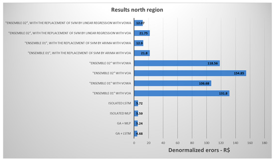
Figure 14.
MSE graph to predict the best PLD results.
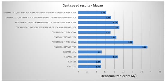
Figure 15.
MSE graph for predicting the best wind speed results.
For a better understanding, the values were “denormalized” using a minimum of R$ 4.0 and a maximum of R$ 684 as references.
The results obtained in the analysis revealed that the GA + LSTM model achieved the best performance compared to the other evaluated models (Figure 14). The second-best result was from the GA + MLP model, with a slight difference from the top performer.
The ensembles that did not use SVM demonstrated better performances.
When comparing different voting methods, it was observed that VOWA achieved the best performance.
For better understanding, the values were “denormalized” using a minimum of 1.15 m/s and a maximum of 10.07 m/s as references.
As evidenced in Figure 15, the GA + LSTM model demonstrated a “higher” performance, with a margin of only 0.01 m/s compared to the second-best model and a distinct difference of 0.29 m/s compared to the third-placed “ensemble 02”, in which SVM was replaced by the linear regression model.
Within the results of the ensembles, “ensemble 02”, which replaced SVM with the linear regression model in VOWA, outperformed not only all the other ensembles but also the individual performances of the members that composed “ensemble 02”.
On this occasion, Table 18 and Table 19 provide a comparison of the highlighted model proposed for forecasting in relation to other published models for wind speed and PLD. The comparative assessment with other models is conducted using the root mean square error (RMSE) criterion to provide a more intuitive interpretation of the results. This is particularly relevant, given that references [52,70,71,72] present their metrics in RMSE. Thus, the analysis is carried out after extracting the square root of mean squared error (MSE) values, aiming for a more direct understanding and consistent comparison with the mentioned references.

Table 18.
Comparison of the proposed forecasting model with other published models for wind speed.

Table 19.
Comparison of the proposed prediction model with other published models for the PLD.
It is crucial to emphasize that this study is focused on one-step-ahead prediction, with wind speed as the predictive variable. To compare with similar research, reference [52] utilizes a four-day training window average for wind prediction, while [70] is dedicated to the forecasting of monthly average time series.
In the context of Table 19, two models were referenced: LSTM and decision tree. The results show error values of 1.2, 32.25, and 82.41, respectively, for these models. Each of these methods demonstrates distinct characteristics in terms of performance, and the analysis of these results provides valuable insights into the suitability of each approach in the specific context of the application at hand.
5. Conclusions
The analysis of this study proposes a methodology that employs a variety of existing algorithms, including adaptations of some, to predict time series related to the Brazilian electrical system. Notably, the combination of deep learning with hyperparameters optimized through the canonical genetic algorithm, using an individual representation, yields good results when compared to the other studied methods.
The objective is to enhance the accuracy of the results through the application of advanced machine learning techniques. In this way, the aim is to achieve more precise and reliable predictions of the price of settlement differences, which is a reference factor for prices in the free energy market in Brazil and renewable energy system planning (wind speed forecasting).
The proposed methodology encompasses the use of machine learning models that incorporate hybrid approaches between genetic algorithm (GA), LSTM, and MLP, as well as the implementation of an ensemble with support vector machines (SVMs), deep learning, and other relevant techniques. Each of these models is trained using data related to the PLD and wind energy. The evaluation of their performances is conducted using common metrics such as mean squared error (MSE).
The results obtained revealed that the GA + LSTM model achieved the best prediction performance compared to the other models, with an error of 4.68 on the PLD dataset and an error of 1.26 on the Macau dataset.
Regarding the implementation of the voting model, which combines the predictions of various models into a single final prediction, it was evaluated using two distinct approaches: voting average (VOA) and voting weighted average (VOWA). The results obtained indicate that weighted average voting shows superior prediction performance compared to voting average. This highlights the importance of taking into consideration the relative contribution of each model to the final prediction.
When individual models (committee members) exhibit superior results to the committee, this discrepancy can be attributed to various factors. The amalgamation of individual models into a committee may fall short of fully capturing the nuances of the data. In this context, tuning hyperparameters to better reflect the performance of each model becomes crucial for enhancing the overall committee outcome, among other considerations. It is essential to emphasize the ongoing pursuit of committee performance improvement, whether through adjustments in weights, training optimization, or the consideration of specific factors from individual models contributing to success.
Hybridizing deep learning, enhanced by optimized hyperparameters through the canonical genetic algorithm and implementing machine committees, has revealed practical implications of great relevance, along with their strengths and weaknesses for consideration.
5.1. Practical Implications
Greater Efficiency in Solving Complex Problems: The combination of these techniques enables more efficient handling of complex problems. Neural networks can offer learning and generalization capabilities, genetic algorithms contribute to optimization and efficient solution search, while machine committees aggregate diverse perspectives and decision-making robustness.
Adaptation to Different Contexts: The combination of these methods can be adjusted to fit different domains or application contexts. This allows for the creation of more flexible and adaptable systems capable of handling variations and changes in data or environments.
5.2. Strengths
Synergy Among Diverse Techniques: The complementarity of neural networks, genetic algorithms, and machine committees allows for exploring synergies between these approaches, taking advantage of their respective strengths, and minimizing individual limitations.
Improved Accuracy and Generalization: The combination of these techniques can result in more precise models with better generalization capabilities, especially when dealing with complex datasets.
Exploration of Optimal and Diverse Solutions: Genetic algorithms can efficiently explore a solution space, while machine committees can provide a variety of opinions, enhancing decision making. This can lead to the discovery of optimal and diverse solutions.
5.3. Weaknesses
Computational Complexity and Costs: The combination of different techniques can increase the complexity of models and require more robust computational resources, resulting in longer processing times and associated costs.
Difficulty in Interpretability: At times, combining various techniques can make the resulting model more challenging to interpret and explain.
Challenges in Parameter Tuning: Optimizing and adjusting the parameters of these combined techniques can be challenging and can require significant expertise and time to find ideal configurations.
Furthermore, it is concluded that electric power forecasting is a topic of significant importance, as evidenced by the abundance of publications dedicated to this subject. This article contributes to the analysis of the use of various machine learning techniques in the Brazilian context. There is a growing trend in the use of hybrid models aimed at achieving more accurate predictions. This approach is crucial to drive the search for solutions that minimize global impacts, incorporating optimization in various aspects such as efficiency and profitability.
Author Contributions
T.C. conceived the idea and wrote the introduction, literature review, materials and methods, results and discussions, and conclusion. R.O. conceived the idea and reviewed the article. All authors have read and agreed to the publication of the article. All authors have read and agreed to the published version of the manuscript.
Funding
The study was supported by the graduate program in electrical engineering (PPGEE) administered by the Federal University of Pará (UFPA).
Data Availability Statement
Data are contained within the article.
Conflicts of Interest
The authors declare no conflicts of interest.
References
- Electricity Trading Chamber. Available online: https://www.ccee.org.br/ (accessed on 5 June 2023). (In Portuguese).
- Gas Emission Estimation System. Available online: https://seeg.eco.br/ (accessed on 5 June 2023). (In Portuguese).
- Ministry of Science, Technology and Innovation. Available online: https://www.gov.br/mcti/pt-br (accessed on 5 June 2023). (In Portuguese)
- Organization for Economic Co-Operation and Development. Available online: https://www.gov.br/economia/pt-br/assuntos/ocde (accessed on 5 June 2023). (In Portuguese)
- Ministry of Mines and Energy. Available online: https://www.gov.br/mme/ (accessed on 11 April 2023). (In Portuguese)
- Infovento. Available online: https://abeeolica.org.br/dados-abeeolica/infovento-29/ (accessed on 13 January 2023). (In Portuguese).
- National Electric Energy Agency. Available online: https://www.gov.br/aneel/ (accessed on 11 April 2023). (In Portuguese)
- Kotyrba, M.; Volna, E.; Habiballa, H. The Influence of Genetic Algorithms on Learning Possibilities of Artificial Neural Networks. Computers 2022, 11, 70. [Google Scholar] [CrossRef]
- Tran, L.; Le, A.; Nguyen, T.; Nguyen, D.T. Explainable Machine Learning for Financial Distress Prediction: Evidence from Vietnam. Data 2022, 7, 160. [Google Scholar] [CrossRef]
- Ambrioso, J.; Brentan, B.; Herrera, M.; Luvizotto, E., Jr.; Ribeiro, L.; Izquierdo, J. Committee Machines for Hourly Water Demand Forecasting in Water Supply Systems. Math. Probl. Eng. 2019, 2019, 9765468. [Google Scholar] [CrossRef]
- Wang, S.; Roger, M.; Sarrazin, J.; Perrault, C. Hyperparameter Optimization of Two-Hidden-Layer Neural Networks for Power Am-plifiers Behavioral Modeling Using Genetic Algorithms. IEEE Microw. Wirel. Compon. Lett. 2019, 29, 802–805. [Google Scholar] [CrossRef]
- Coordination for the Improvement of Higher Education Personnel. Available online: https://www-periodicos-capes-gov-br.ezl.periodicos.capes.gov.br/index.php?/ (accessed on 3 October 2023). (In Portuguese)
- Bhattacharyya, S. Markets for electricity supply. In Energy Economics, 2nd ed.; Springer: London, UK, 2019; pp. 699–733. [Google Scholar]
- Maciejowska, K. Assessing the impact of renewable energy sources on the electricity price level and variability—A quantile regression approach. Energy Econ. 2020, 85, 104532. [Google Scholar] [CrossRef]
- Junior, F. Direct and Recurrent Neural Networks in Predicting the Price of Short-Term Electricity in the Brazilian Market. Master’s Thesis, Federal University of Pará, Belém, PA, Brazil, 2016. (In Portuguese). [Google Scholar]
- Ribeiro, M.H.D.M.; Stefenon, S.F.; de Lima, J.D.; Nied, A.; Mariani, V.C.; Coelho, L.d.S. Electricity Price Forecasting Based on Self-Adaptive Decomposition and Heterogeneous Ensemble Learning. Energies 2020, 13, 5190. [Google Scholar] [CrossRef]
- Corso, M.P.; Stefenon, S.F.; Couto, V.F.; Cabral, S.H.L.; Nied, A. Evaluation of methods for electric field calculation in transmission lines. IEEE Lat. Am. Trans. 2018, 16, 2970–2976. [Google Scholar] [CrossRef]
- Filho, J.; Affonso, C.; Oliveira, R. Energy price prediction multi-step ahead using hybrid model in the Brazilian market. Electr. Power Syst. Res. 2014, 117, 115–122. [Google Scholar] [CrossRef]
- Hong, T.; Pinson, P.; Wang, Y.; Weron, R.; Yang, D.; Zareipour, H. Energy Forecasting: A Review and Outlook. IEEE Open Access J. Power Energy 2020, 7, 376–388. [Google Scholar] [CrossRef]
- Ozcanli, A.; Yaprakdal, F.; Baysal, M. Deep learning methods and applications for electrical power systems: A comprehensive review. Energy Res. 2020, 44, 7136–7157. [Google Scholar] [CrossRef]
- Abedinia, O.; Lotfi, M.; Bagheri, M.; Sobhani, B.; Shafie-khah, M.; Catalão, J. Improved EMD-Based Complex Prediction Model for Wind Power Forecasting. IEEE Open Access J. Power Energy 2020, 11, 2790–2802. [Google Scholar] [CrossRef]
- Heydari, A.; Nezhad, M.; Pirshayan, E.; Garcia, D.; Keynia, F.; Santoli, L. Short-term electricity price and load forecasting in isolated power grids based on composite neural network and gravitational search optimization algorithm. Appl. Energy 2020, 277, 115–503. [Google Scholar] [CrossRef]
- Chen, W.; Chen, Y.; Tsangaratos, P.; Llia, L.; Wang, X. Combining Evolutionary Algorithms and Machine Learning Models in Landslide Susceptibility Assessments. Remote Sens. 2020, 12, 3854. [Google Scholar] [CrossRef]
- Luo, X.; Oyedele, L.; Ajayi, A.; Akinade, O.; Delgado, J.; Owolabi, H.; Ahmed, A. Genetic algorithm-determined deep feedforward neural network architecture for predicting electricity consumption in real buildings. Energy AI 2020, 2, 100015. [Google Scholar] [CrossRef]
- Alencar, D. Hybrid Model Based on Time Series and Neural Networks for Predicting Wind Energy Generation. Ph.D. Thesis, Federal University of Pará, Belém, PA, Brazil, 2018. (In Portuguese). [Google Scholar]
- Junior, K. Genetic Algorithms and Deep Learning Based on Long Short-Term Memory (LSTM) Recurrent Neural Networks for Medical Diagnosis Assistance. Doctoral Thesis, University of São Paulo, Ribeirão Preto, SP, Brazil, 2023. [Google Scholar] [CrossRef]
- Li, W.; Zang, C.; Liu, D.; Zeng, P. Short-term Load Forecasting of Long-short Term Memory Neural Network Based on Genetic Algorithm. In Proceedings of the 4th IEEE Conference on Energy Internet and Energy System Integration (EI2), Wuhan, China, 30 October–1 November 2020. [Google Scholar] [CrossRef]
- Zulfiqar, M.; Rasheed, M.B. Short-Term Load Forecasting using Long Short Term Memory Optimized by Genetic Algorithm. In Proceedings of the IEEE Sustainable Power and Energy Conference (iSPEC), Perth, Australia, 4–7 December 2022. [Google Scholar] [CrossRef]
- Bendali, W.; Saber, I.; Bourachdi, B.; Boussetta, M.; Mourad, Y. Deep Learning Using Genetic Algorithm Optimization for Short Term Solar Irradiance Forecasting. In Proceedings of the Fourth International Conference on Intelligent Computing in Data Sciences (ICDS), Fez, Morocco, 21–23 October 2020. [Google Scholar] [CrossRef]
- Al Mamun, A.; Hoq, M.; Hossain, E.; Bayindir, R. A Hybrid Deep Learning Model with Evolutionary Algorithm for Short-Term Load Forecasting. In Proceedings of the 8th International Conference on Renewable Energy Research and Applications (ICRERA), Brasov, Romania, 3–6 November 2019. [Google Scholar] [CrossRef]
- Huang, C.; Karimi, H.R.; Mei, P.; Yang, D.; Shi, Q. Evolving long short-term memory neural network for wind speed forecast-ing. Inf. Sci. 2023, 632, 390–410. [Google Scholar] [CrossRef]
- Shahid, F.; Zameer, A.; Muneeb, M. A novel genetic LSTM model for wind power forecast. Energy 2021, 223, 120069. [Google Scholar] [CrossRef]
- ul Islam, B.; Baharudin, Z.; Nallagownden, P.; Raza, M.Q. A Hybrid Neuro-Genetic Approach for STLF: A Comparative Analy-sis of Model Parameter Variations. In Proceedings of the IEEE 8th International Power Engineering and Optimization Conference (PEOCO2014), Langkawi, Malaysia, 24–25 March 2014. [Google Scholar] [CrossRef]
- Izidio, D.M.F.; de Mattos Neto, P.S.G.; Barbosa, L.; de Oliveira, J.F.L.; Marinho, M.H.d.N.; Rissi, G.F. Evolutionary Hybrid Sys-tem for Energy Consumption Forecasting for Smart Meters. Energies 2021, 14, 1794. [Google Scholar] [CrossRef]
- Elsken, T.; Metzen, J.; Hutter, F. Neural Architecture Search. Autom. Mach. Learn. 2019, 63–77. [Google Scholar] [CrossRef]
- Wang, S.; Zhang, N.; Wu, L.; Wang, Y. Wind speed forecasting based on the hybrid ensemble empirical mode decomposition and GA-BP neural network method. Renew. Energy 2016, 94, 629e636. [Google Scholar] [CrossRef]
- Cao, Y.; Liu, G.; Luo, D.; Bavirisetti, D.P.; Xiao, G. Multi-timescale photovoltaic power forecasting using an improved Stacking ensemble algorithm based LSTM-Informer model. Energy 2023, 283, 128669. [Google Scholar] [CrossRef]
- Shi, J.; Teh, J. Load forecasting for regional integrated energy system based on complementary ensemble empirical mode de-composition and multi-model fusion. Appl. Energy 2024, 353, 122146. [Google Scholar] [CrossRef]
- Wu, Z.; Wang, B. An Ensemble Neural Network Based on Variational Mode Decomposition and an Improved Sparrow Search Algorithm for Wind and Solar Power Forecasting. IEEE Access 2021, 9, 166709. [Google Scholar] [CrossRef]
- Ribeiro, M.; da Silva, G.; Canton, C.; Fraccanabbi, N.; Mariani, C.; Coelho, S. Electricity energy price forecasting based on hybrid multi-stage heterogeneous ensemble: Brazilian commercial and residential cases. In Proceedings of the International Joint Conference on Neural Networks (IJCNN), Glasgow, UK, 19–24 July 2020. [Google Scholar] [CrossRef]
- Doan, Q.; Le, T.; Thai, D. Optimization strategies of neural networks for impact damage classification of RC panels in a small dataset. Appl. Soft Comput. 2021, 102, 107100. [Google Scholar] [CrossRef]
- Kadhim, Z.; Abdullah, H.; Ghathwan, K. Artificial Neural Network Hyperparameters Optimization: A Survey. Int. J. Online Biomed. Eng. 2022, 18, 15. [Google Scholar] [CrossRef]
- Masís, A.; Cruz, A.; Schierholz, M.; Duan, X.; Roy, K.; Yang, C.; Donadio, R.; Schuster, C. ANN Hyperparameter Optimization by Genetic Algorithms for Via Interconnect Classification. In Proceedings of the IEEE 25th Workshop on Signal and Power Integrity (SPI), Siegen, Germany, 10–12 May 2021. [Google Scholar]
- Phyo, P.; Byun, Y. Hybrid Ensemble Deep Learning-Based Approach for Time Series Energy Prediction. Symmetry 2021, 13, 1942. [Google Scholar] [CrossRef]
- Yang, X. Nature-Inspired Optimization Algorithms, 2nd ed.; Academic Press: London, UK, 2020; pp. 107–118. [Google Scholar]
- Kochenderfer, M.; Wheeler, T. Algorithms for Optimization, 1st ed.; Mit Press: London, UK, 2019; pp. 147–162. [Google Scholar]
- Garbin, C.; Zhu, X.; Marques, O. Dropout vs. batch normalization: An empirical study of their impact to deep learning. Multimed. Tools Appl. 2020, 79, 12777–12815. [Google Scholar] [CrossRef]
- Akhtar, S.; Shahzad, S.; Zaheer, A.; Ullah, H.; Kilic, H.; Gono, R.; Jasinski, M.; Leonowicz, Z. Short-Term Load Forecasting Models: A Review of Challenges, Progress, and the Road Ahead. Energies 2023, 16, 4060. [Google Scholar] [CrossRef]
- Kurani, A.; Doshi, P.; Vakharia, A.; Shah, M. A Comprehensive Comparative Study of Artificial Neural Network (ANN) andSupport Vector Machines (SVM) on Stock Forecasting. Ann. Data Sci. 2023, 10, 183–208. [Google Scholar] [CrossRef]
- Dagoumas, A.; Koltsaklis, N. Review of models for integrating renewable energy in the generation expansion planning. Appl. Energy 2019, 242, 1573–1587. [Google Scholar] [CrossRef]
- Hur, Y. An Ensemble Forecasting Model of Wind Power Outputs based on Improved Statistical Approaches. Energies 2020, 13, 1071. [Google Scholar] [CrossRef]
- Carneiro, T.; Rocha, P.; Carvalho, P.; Ramírez, L. Ridge regression ensemble of machine learning models applied to solar and wind forecasting in Brazil and Spain. Appl. Energy 2022, 314, 118936. [Google Scholar] [CrossRef]
- Sagi, O.; Rokach, L. Ensemble learning: A survey. WIREs Data Mining Knowl Discov. 2018, 8, e1249. [Google Scholar] [CrossRef]
- Solano, E.S.; Affonso, C.M. Solar Irradiation Forecasting Using Ensemble Voting Based on Machine Learning Algorithms. Sustainability 2023, 15, 7943. [Google Scholar] [CrossRef]
- Phyo, P.-P.; Byun, Y.-C.; Park, N. Short-Term Energy Forecasting Using Machine-Learning-Based Ensemble Voting Regression. Symmetry 2022, 14, 160. [Google Scholar] [CrossRef]
- Alymani, M.; Mengash, H.A.; Aljebreen, M.; Alasmari, N.; Allafi, R.; Alshahrani, H.; Elfaki, M.A.; Hamza, M.A.; Abdelmageed, A.A. Sustainable residential building energy consumption forecasting for smart cities using optimal weighted voting ensemble learning. Sustain. Energy Technol. Assess. 2023, 57, 103271. [Google Scholar] [CrossRef]
- Christoph, E.; Raviv, E.; Roetzer, G. Forecast Combinations in R using the ForecastComb Package. R J. 2019, 10, 262. [Google Scholar] [CrossRef]
- Villanueva, W. Committee on Machines in Time Series Prediction. Master’s Thesis, Campinas State University, Campinas, SP, Brazil, 2006. (In Portuguese). [Google Scholar]
- Zhou, Q.; Wang, C.; Zhang, G. A combined forecasting system based on modified multi-objective optimization and sub-model selection strategy for short-term wind speed. Appl. Soft Comput. 2020, 94, 106463. [Google Scholar] [CrossRef]
- Lv, S.; Wang, L.; Wang, S. A Hybrid Neural Network Model for Short-Term Wind Speed Forecasting. Energies 2023, 16, 1841. [Google Scholar] [CrossRef]
- Wang, L. Advanced Multivariate Time Series Forecasting Models. J. Math. Stat. 2018, 14, 253–260. [Google Scholar] [CrossRef]
- Conte, T.; Santos, W.; Nunes, L.; Veras, J.; Silva, J.; Oliveira, R. Use of ARIMA and SVM for forecasting time series of the Brazilian electrical system. Res. Soc. Dev. 2023, 12, 3. [Google Scholar] [CrossRef]
- Bitirgen, K.; Filik, U. Electricity Price Forecasting based on XGBooST and ARIMA Algorithms. J. Eng. Res. Technol. 2020, 1, 7–13. [Google Scholar]
- National Environmental Data Organization System (SONDA). Available online: http://sonda.ccst.inpe.br/basedados/ (accessed on 11 April 2023). (In Portuguese).
- Puheim, M.; Madarász, L. Normalization of inputs and outputs of neural network based robotic arm controller in role of inverse kinematic model. In Proceedings of the IEEE 12th International Symposium on Applied Machine Intelligence and Informatics (SAMI), Herl’any, Slovakia, 23–25 January 2014. [Google Scholar] [CrossRef]
- Lee, S.; Kim, J.; Kang, H.; Kang, D. Genetic Algorithm Based Deep Learning Neural Network Structure and Hyperparameter Optimization. Appl. Sci. 2021, 11, 774. [Google Scholar] [CrossRef]
- Géron, A. Hands-on Machine Learning with Scikit-Learn, Keras, and TensorFlow: Concepts, Tools, and Techniques to Build Intelligent Systems, 2nd ed.; O’Reilly Media: Sebastopol, CA, USA, 2020; pp. 62–70. [Google Scholar]
- Carvalho, A.; Gama, J.; Lorena, A.; Faceli, K. Artificial Intelligence: A Machine Learning Approach, 1st ed.; LTC: Rio de Janeiro, Brazil, 2011; p. 394. (In Portuguese) [Google Scholar]
- Bradshaw, A. Electricity Market Reforms and Renewable Energy: The Case of Wind and Solar in Brazil. Ph.D. Thesis, Columbia University, New York, NY, USA, 2018. [Google Scholar]
- Camelo, H.; Lucio, P.; Junior, J.; Carvalho, P. Time Series Forecasting Methods and Hybrid Modeling both Applied to Monthly Average Wind Speed for Northeastern Regions of Brazil. Braz. Meteorol. Mag. 2017, 32, 565–574. (In Portuguese) [Google Scholar] [CrossRef][Green Version]
- Belentani, Y. Short-Term Market Energy Price Forecasting: A Combined Analysis of Time Series and Artificial Neural Networks. Master’s Thesis, São Paulo University, São Paulo, Brazil, 2023. (In Portuguese). [Google Scholar]
- Santos, C.; Silva, L.; Castro, R.; Marques, R. Application of machine learning to project the hourly price for settlement of differences to support electricity trading strategies. Braz. Energy Mag. 2022, 28, 243–279. [Google Scholar] [CrossRef]
Disclaimer/Publisher’s Note: The statements, opinions and data contained in all publications are solely those of the individual author(s) and contributor(s) and not of MDPI and/or the editor(s). MDPI and/or the editor(s) disclaim responsibility for any injury to people or property resulting from any ideas, methods, instructions or products referred to in the content. |
© 2024 by the authors. Licensee MDPI, Basel, Switzerland. This article is an open access article distributed under the terms and conditions of the Creative Commons Attribution (CC BY) license (https://creativecommons.org/licenses/by/4.0/).