Abstract
In biology, respiratory quotient (RQ) is defined as the ratio of CO2 moles produced per mole of oxygen consumed. Recently, Annamalai et al. applied the RQ concept to engineering literature to show that CO2 emission in Giga Tons per Exa J of energy = 0.1 ∗ RQ. Hence, the RQ is a measure of CO2 released per unit of energy released during combustion. Power plants on earth use a mix of fossil fuels (FF), and the RQ of the mix is estimated as 0.75. Keeling’s data on CO2 and O2 concentrations in the atmosphere (abbreviated as atm., 1991–2018) are used to determine the average RQGlob of earth as 0.47, indicating that 0.47 “net” moles of CO2 are added to which means that there is a net loss of 5.6 kg C(s) from earth per mole of O2 depleted in the absence of sequestration, or the mass loss rate of earth is estimated at 4.3 GT per year. Based on recent literature on the earth’s tilt and the amount of water pumped, it is speculated that there could be an additional tilt of 2.7 cm over the next 17 years. While RQ of FF, or biomass, is a property, RQGlob is not. It is shown that the lower the RQGlob, the higher the acidity of oceans, the lesser the CO2 addition to atm, and the lower the earth’s mass loss. Keeling’s saw-tooth pattern of O2 is predicted from known CO2 data and RQGlob. In Part II, the RQ concept is expanded to define energy-based RQGlob,En, and adopt the CO2 and O2 balance equations, which are then used in developing the explicit relations for CO2 distribution amongst atm., land, and ocean, and the RQ-based results are validated with results from more detailed literature models for the period 1991–2018.
1. Introduction
According to Biology Online [1], life is defined as “a distinctive characteristic of a living organism from a dead organism or non-living thing, as specifically distinguished by the capacity to grow, metabolize, respond (to stimuli), adapt, and reproduce”. On the other hand, non-biological systems (NBS) include thermal systems (e.g., heat engines, power plants, etc.) which convert the chemical energy of fossil fuels (FF) into work via rapid oxidation or combustion. The NBS “breathe” in oxygen, oxidizes FF, which includes natural gas, oil, and coal, and “breathe” out CO2 and H2O. The metabolism of nutrients (or fuels) in many biological systems (including BS, humans, land and ocean animals, plants, etc.) involves slow oxidation, consuming oxygen, and then breathing out CO2. In biology, the ratio of moles of CO2 produced to O2 moles used in the release of energy is called the respiration quotient (RQ). Like NBS and BS, the earth undergoes a breathing cycle, but with a difference. While NBS, particularly humans, cannot naturally produce oxygen, terrestrial ecosystems include trees and plants on land, and phytoplankton (PP) in oceans “breathe” in CO2 and “breathe” out O2 under photosynthesis (PS), where C is stored as the growth mass of biomass. In addition, biomass undergoes a “respiration” process, which is used to oxidize sugars for life-sustaining functions during the growth of biomass [2,3]. In addition to CO2 from FF, the dead organic matter releases CO2 ≈ 50 GT/year). The net primary product (NPP) of C i during the photosynthesis is the difference between the gross primary production (GPP, ≈120 GT of C/year and the C used in the respiration process (≈60 GT of C/year) and hence the NPP during photosynthesis is about 60 GT of C/year while decomposition of biomass is about 50 GT/year. Thus, the NEP of the ecosystem is 10 GT/year [4]. It is apparent that biomass serves as a CO2 sink and an O2 source in the growth of biomass, (i.e., CO2 is split into C(s) and O2). As used here, the term biomass represents both terrestrial and ocean-based plants. For biomass growth, the CO2 literature uses a photosynthetic quotient (PQ = O2 mols produced/CO2 mols used), which is the inverse of RQ used in biology and various other terms (more details in Section 3).
In addition, CO2 is mainly released from the combustion of FF (e.g., coal, oil, gasoline, diesel, kerosene, and natural gas) in power plants, land uses, and industrial processes; the corresponding decrease in O2 in the atm is due to the consumption of fossil fuels. The CO2 emissions reached about 36.3 giga tons (GT) of CO2 in 2021, and a majority (almost 80%) of the total carbon emissions have been due to coal and liquid fuels, with about 20% from the combustion of gaseous fuels [5].
Apart from biomass, which serves as the CO2 sink, CO2 is also stored in the ocean. The difference between CO2 produced and CO2 sinks via biomass and ocean storage results in the accumulation of CO2 in the atmosphere {d[CO2]/d}atm, and the difference between O2 consumed for oxidation of FF and O2 produced by biomass results in the net depletion of O2 from the atmosphere {d[O2]/dt}atm. Since 1958, Keeling has monitored this change in CO2 and O2 concentrations by taking air samples from the atm over several decades and presenting Keeling’s curves, which exhibit a saw tooth pattern for both CO2 and O2. These saw tooth patterns and the inverse relation between CO2 and O2 (i.e., CO2 increases when O2 decreases in the atm and vice versa) reveal certain similarities to the RQ concept in biology. The biology literature assumes that the energy release per unit mole of oxygen, or higher heating value per unit mole, or Peta mole of oxygen {HHVO₂), is constant at about 448 Exa J per Peta mole of O2 consumed for oxidation. The RQ concept was recently extended to engineering literature [6,7]. It was shown that the CO2 released in giga tons per unit Exa J is equal to 0.1 ∗ RQ (more details in Section 3.3.1). This relation was also used to estimate the CO2 tax per km or mile driven rather than using the weight of the vehicle for taxation as currently done in the EU [6]. The lower the RQ (e.g., natural gas with RQ = 0.5), the lower the CO2 emitted, and the higher the RQ (e.g., coal, RQ ≈ 1), the higher the CO2 emitted for the same energy released. In order to minimize the amount of CO2 added to the atm, it is of interest to select FF, which has the lowest amount of CO2 released for fixed energy release.
2. Literature Review
The literature review is divided into the following sections: (i) CO2 source from FF and other global warming gases, (ii) Keeling’s data on CO2 and O2 in the atmosphere (atm), (iii) CO2 and global warming, (iv) CO2 sources and sinks, O2 sources and sinks, and models, and (v) the need for current work.
2.1. Fosssil Fuel, Land Use and CO2
Large quantities of CO2 released from the combustion of FF (about 87 % of CO2) play a major role in climate forcing [8]. Further CO2 is also released due to the land use (LU, 13 %, fire, deforestation, domestic wood consumption, decomposition of dead wood in soil, etc.) by humans. The combined CO2 from FF and LU will be referred to as CO2 from FFLU. Global warming gases include CO2, CH4, N2O [9], and chlorofluorocarbons (CFC) with various degrees of global warming potential (GWP). The GWP of biofuels was evaluated by Holtsmark and compared against the impacts of fossil fuels [10]. Biomass and other renewable fuels (e.g., ethanol produced from plant materials), including nutrients consumed by BS, are considered to be carbon neutral, and hence the CO2 released due to the oxidation of renewable fuels is not considered in the carbon footprint, while the C emitted during the combustion of FF is accounted for in the carbon footprint. Due to anthropogenic activities, each fuel has its own share of global warming, irrespective of whether the fuel is renewable or non-renewable. For the period 1950–1982, Boden et al. [5] estimated the emission of CO2 using the fuel production data, and C oxidized to CO2. The impact of residential energy consumption on GHG emissions and policies that can be implemented to reduce energy utilization were reviewed by Nejat et al. [11].
2.2. Keeling’s Data on CO2 and O2 and Saw Tooth Pattern
Using monthly data from weather stations close to volcano Mauna Loa, Hawaii (NO AA Global Monitoring Lab, Mauna Loa Observatory (MLO), North flank of Mauna Loa Volcano, Hawaii, elevation: 3397 m above sea level (far from human population) on CO2 and O2 (1960–2021), Keeling plotted CO2 and O2 vs. year (Figure 1), which is known as Keeling’s curve [12,13]. The curves reveal the asynchronous “choreography between atmospheric CO2 and O2” and the saw-tooth pattern on CO2 and O2. Instead of “per meg” units of Keeling, ppm (4.8 per MEG = 1 ppm) is used for CO2 concentrations in the current text. Figure 1 reveals a cyclic saw-tooth pattern of small peaks and valleys (note: captions of figures contain more information so that text could be reduced). Balkanski et al. [14] attribute the CO2 cycle to terrestrial (land) biotic activity. Particularly during fall and winter (FW, Fall: September, October, and November; Winter: December, January, and February), the release of CO2 due to the combustion of fossil fuels and the sink of oxygen from the atm. dominate the CO2 sink and O2 production for the growth of biomass. Thus, during FW, ΔCO2 > 0 and ΔO2 < 0. The reverse happens in spring and summer (SS, Spring: March, April, May; Summer: June, July, August); the sink of CO2 and production of O2 via biomass growth and limited outgassing of O2 from the ocean (due to warm temperatures) dominate the CO2 source and O2 sink for energy release from power plants, resulting in ΔCO2 < 0 and ΔO2 > 0 in SS [15]. The amplitude of CO2 oscillation is about 6 ppm. The net effect of FW and SS behaviors is positive production of CO2 per year, resulting in an increase of atmospheric CO2 in ppm.

Figure 1.
The saw-tooth pattern of CO2 and O2 concentrations in earth’s atmosphere. Adopted from Ref. [16]. Night-time CO2 concentration > day-time CO2 concentration due to photosynthesis during daytime. Change in O2 expressed as δ(O2/N2) (per meg) by Keeling [16]; they have negative values; O2 in ppm = per meg units ∗ 0.2096, or 4.8 per megs = 1 ppm of O2; also see Ref. [17]. Air in atm: 1.77 × 10⁵ Peta Moles. 1 ppm of any species in atm = 0.177 Peta Moles. Between 1960 and 2019, δ(O2/N2) decreased by 700 per meg, implying decrease of 147 ppm of O2. The referenced oxygen concentration in 1960 was 209,640 ppm. The fluctuations (small peaks and valleys) in CO2 each year are due to seasonal changes from FW to SS. See data collection [16]. The CO2 average for 2022 was 417.1 ppm (NOAA). Since 2000, almost 75% of the increase in CO2 is due to fossil fuel combustion. If the 2021 CO2 level (415.1 ppm) needs to be restored to the 2000 level (369.7 ppm), one must sequester CO2 mass of 353 GT.
2.3. CO2 and Global Warming
The CO2 record shows that the normal level of CO2 for centuries was about 300 ppm; however, it reached 414.7 ppm in 2021 and 424 ppm in May 2023 [18]. An increase of 2 ppm of CO2/year (i.e., almost 15.6 GT of CO2 added to atm) is related to a global warming rate of 0.0125 °C/year [19]. The synchronous dance between CO2 and Antarctic temperatures is illustrated in Figure 2, while Figure 3 shows the temperature since 1875. The rising global temperature of the earth is shown to reduce the PS process; hence, by 2040, CO2 sink due to biomass growth will be reduced by almost 50% [20].
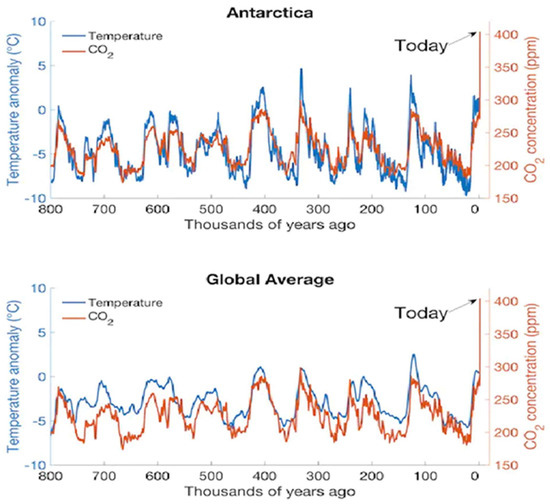
Figure 2.
Correlation between CO2 and atmospheric temperature anomaly (deviation from long-term (30 years) average temperature) in Antarctica (measured from European Project for Ice Coring in Antarctica (EPICA) Dome C ice core sample containing trapped air} and global temperature anomaly; see Ref. [21] for global average surface temperature data. The CO2 levels fluctuated between 200 and 280 ppm (mean: 240 ppm) for several thousands of years before 2000. The atmospheric temperature fluctuates in synchrony with CO2 fluctuations for both global average and Antarctica. (Additional Refs: Jouzel et al., 2007 [22]; Lüthi et al. [23]) For records on CO2 and temperature 800,000 years before the present, see refs. [22,23,24]. In March 2022, the temperature in Eastern Antarctica spiked by 39 °C (102.2 °F) above the monthly average of −45 °C.
The relationship between CO2, warming temperature rise, saturation pressure of water vapor, and hence the increasing number of hurricanes, wildfires, etc., is well established [25]. There is also increased seaweed (Sargassum, which smells like rotten eggs–due to hydrogen sulfide) growth due to global warming and rainfall. Assuming ocean temperatures are the same as the global average temperature, the author estimated the variation in saturation pressure, which is shown in Figure 3. Assuming the % increase in hurricanes from 2012 to 2022 is proportional to the % increase in saturation pressure (about 12%). The data from the autopiloted Saildrone Explorer SD 1045 boat indicated a 10% increase in hurricanes and an 8% increase in storms [26], but rain increased only by 1.3% per K rise. The increased ocean temperature will also result in the release of O2 from oceans (a decrease of 0.2–0.5% per year from oceans). The warmer the ocean, the more vapor in a region and the lesser the barometric pressure, resulting in a higher wind velocity and faster growth of hurricanes [27].

Figure 3.
Relation between the global temperature (primary axis, solid line) and the saturation pressure of water (secondary axis, dashed line); temperature data taken from Ref. [28] and pasted onto EXCEL sheet. Global Average T in °C = 2.326 × 10⁻⁴ ∗ year2 − 0.02539 ∗ year + 11.39, Year: (Specified year-1875) Psat by the author using ln(Psat) = A − B/(T + D), Psat in bar, T in °C, A = 12.22, B = 4120.6, D = 237.9: For 2002, temperature rise per year = 0.044 °C/year, and 0.44 °C/decade. Increasing global temperature causes increasing saturation pressure (Psat); evaporation rate is proportional to Psat.
2.4. CO2 Sources and Sinks, O2 Sources and Sinks, and Models
There is extensive literature on CO2 emissions and CO2 distribution amongst atm, land, and ocean biomasses and oceans. The CO2 sinks and O2 sources are mainly land biomass plants, trees, and ocean PP and CO2 sinks via ocean storage. Zhu et al. used Integrated Biosphere Simulator or global vegetation model to estimate the effects of climate change and CO2 fertilization on CO2 budget at the local subtropical area of China covered with evergreen forest [29].
The global carbon project summarizes several models for the global C budget: (Table 4 in Ref. [30]): (i) Model for CO2 via land use [31], (ii) Computer model for CO2 flux from land to atm, CO2 sink from global vegetation (land-based biomass [32]), which includes growth function models, (iii) Global ocean bio-geochemistry models, and (iv) Ocean CO2 flux model. Terhaar et al. proposed a new model—An observation-based estimate of ocean carbon sink [33,34]. Gloege et al. modeled ocean uptake by estimating the CO2 flux across the air-sea interface using iterative global ocean biogeochemical models (GOBMs), which include ocean circulation. For the first guess, they use results from earlier models. Li et al. proposed an emission-driven earth system model for predicting the variations in the global carbon budget (GCB) [35] and presented variations in the GCB (1970–2018). Yakir et al. summarizes the use of carbonyl sulfide (COS) as a tracer gas to measure changes in CO2 uptake via PS [36]. To improve the circulation of CO2 sinks in the ocean, artificial deep-water pumping is recommended, and models are presented in ref. [37].
This model details the capture of CO2 in terms of C-N-P ratios, particularly for micro- and macro-algae-based biomass in conditions ranging from tropical to subpolar oceans. Li’s model of land and oceanic sinks is based on the oxygen budget [38]. Zhu et al. used Integrated Biosphere Simulator or global vegetation model to estimate the effects of climate change and CO2 fertilization on CO2 budget at the local subtropical area of China covered with evergreen forest [29]. Control of climate change requires that CO2 emissions are minimized and CO2 sinks are maximized, with the ultimate goal of ‘net-zero’ emissions as per the Paris Agreement [39].
Most of these models require extensive computation tools to estimate CO2 sinks in GT/year for land and ocean sinks, but they are probably more accurate since they account for temperature, soil conditions, ocean circulation, etc. These models were checked by comparing the results for total CO2 capture by atm, land and ocean with CO2 release by FFLU. Hence, there is always a carbon imbalance when CO2 budget analysis is conducted [40]. None of the literature contains explicit relations for CO2 sinks amongst the atmosphere, land, and ocean in terms of the RQ of FF and BM. Those relations provide (i) the first guess for the iterative models and (ii) the governing parameters that affect CO2 distributions. Further, the present model uses CO2 and O2 balance, and hence there is no C imbalance in the current model. While the NASA website [41] contains curve fits to a saw tooth pattern using a polynomial function (quadratic and cubic) with the addition of a sinusoid with time ‘t’ elapsed in years since 1982, the current work uses the RQ method to explain the saw tooth pattern of O2 given CO2 data. Thus, the goal of the current work is to make use of Keeling’s data on CO2 and O2, along with known RQ values of FF and land and ocean biomasses to obtain simple, explicit results for CO2 distribution in GT/year and distribution as a % of total CO2 released via FFLU. In order to achieve the above goals, Part I provides an overview of the RQ concept, a tabulation of the RQ values of FF and BM, and a presentation of global RQ. Part II presents the CO2 and O2 balances and the results for the distribution of CO2 sinks amongst atm, biomasses (land and ocean), and ocean water.
The specific objectives for Part I, methodology, results, and discussion are briefly summarized below:
(i) Perform a brief overview of RQ in biology and engineering and its relation to terms used in conventional CO2 and photosynthesis (PS) literature, (ii) Relate RQ to CO2 in Giga Tons (GT) per unit energy released, (iii) Use the reported data on CO2 emissions in GT and fossil energy in Exa J to estimate the RQ of the mix of fossil fuels (RQFF) used worldwide (gas, liquid, and coal), (iv) Use Keeling’s data on CO2 and O2 in the atm and curve fit the data using linear and quadratic fits, and (v) Define and estimate the global respiratory quotient (RQGlob) of “breathing” planet earth and its significance for the CO2 addition to the atm and CO2 storage in the oceans.
3. Materials and Methods
The methodology consists of the following: (i) the RQ concept for CO2 sources (FF combustion, Section 3.1) and values of RQ for FF, which are properties of FF (ii) RQ concept for CO2 sinks (biomasses, Section 3.2), (iii) comparison of RQ with terms used in PS literature, (iv) RQ values for FF and biomasses and the relations between CO2 in tons per unit energy release, and RQ, (v) RQ of FF for CO2 sources under complete combustion (FF in power plants and automobile engines) and incomplete combustion (oil and gas flares), (vi) Relations between CO2 in tons per unit energy input and RQ of biomass for CO2 sinks, (vii) RQFFLU for the CO2 released from both FF and land use (LU) and RQ of a mix of various types of FF, and (viii) definition of Global RQ {RQGlob} for planet earth, a non-property, using Keeling’s data. Section 4 presents the results for (i) the RQ of the fossil fuel mix used worldwide, (ii) curve fit constants for linear and quadratic fits of Keeling’s data on CO2 and O2, and (iii) an estimation of RQGlob, physical meaning of RQGlob and its implications on CO2 emissions in the atmosphere, atmospheric pressure, mass loss of earth due to mining of FF, and prediction of saw tooth pattern of O2 from given CO2 data and RQGlob.
3.1. Respiratory Quotient (RQ) fr CO2 Sources
3.1.1. Respiratory Quotient (RQ)
The biology literature describes the breathing and overall metabolic processes of BS in terms of the respiratory quotient (RQ), defined as:
where RQnut is the RQ of nutrient s a property, NCO₂,nut is the number of moles of CO2 released when nutrient is oxidized, NC,nut is the number of C atoms in the nutrient, and NO2,nut is the number of moles of O2 used in oxidation.
Caution: a few of the references in both biology and CO2 literature (e.g., [42,43]) use the inverse definition (i.e., O2 moles used/CO2 moles released) for the RQ, and the results in those manuscripts must be interpreted accordingly. For humans or any BS-oxidizing nutrients (glucose C6H12O6, carbohydrate (CH), fat (F), and proteins (P)) produced by the digestive system from food intake, the RQ can be estimated from the chemical formula of the three nutrients [44]:
C6H12O6 + 6 O2 → 6 CO2 + 6 H2O, HHVO2 = 469 kJ/mole O2, RQ = 1
Dividing by 6, one can write the above equation on a unit carbon formula (UCF) basis:
with UCF represented by CH2O, the higher heating value of fuel (HHV) = 2813 kJ/mole of C6H12O6 or HHV = 402.3.1 kJ/mole of CH2O, HHVO2, the energy released per mole of O2 used = 2813/6 = 469 kJ per mole of O2. The =RQ of 1 for glucose indicates that 1 mole of CO2 is released for every mole of O2 used in the oxidation of CH within the body of BS. For the oxidation of fat (C16H32O2), RQ = 0.7. Humans use a mix of CH (RQ = 1) and F (RQ = 0.7); hence, typically, 0.7 ≤ RQ ≤ 1 for a mix of nutrients metabolized. On the other hand, the RQ can also be determined from the analysis of nasal exhaust gas (or automobile exhaust gas); hence, one can determine the % of fat oxidized in the mix of CH and F [45]. The same methodology is adopted for the RQ of thermal power plants when a mix of natural gas, oil, and coal is used globally. For internal combustion engines (automobiles, gas turbines, etc.) fired with any HC liquid fuels or HC mixed with ethanol, the exhaust gas can yield RQ values [7]. Note that RQ, as defined in Equation (1), is a property of fuel whe fuel is used in a thermal system.
CH2O + 1 O2 → 1 CO2 + 1 H2O, HHVO₂ = 469 kJ/mole O2, RQ = 1
3.1.2. Significance of Respiratory Quotient (RQ) and RQ Values for Nutrients and Fuels
Why is RQ important for humans and planet earth? The CO2 released from the metabolism of nutrients in the cells of various organs within a human is collected by the bloodstream, which transfers CO2 to alveoli in the lungs for eventual nasal exhaust. Typically, the normal CO2 in veins is at partial pressure pCO2 (40 mm Hg or 1.2 milli-moles/L). Thus, for seniors with respiratory acidosis (when all CO2 cannot be breathed out, the blood becomes acidic due to CO2 storage exceeding 1.3 milli mole/L) with higher levels of pCO2, a diet with a low RQ (i.e., fat [46]) is recommended [47,48,49,50,51]. Note that during acidosis, the RQ of nasal exhaust (RQvent = CO2 ventilated/O2 consumed) is a non-property < RQnut, which is normally about 0.8. While RQnut is a property of a nutrient or mix of nutrients that can be tabulated (e.g., Table 1), RQvent is not since it depends upon blood capacity and, hence, how much CO2 is stored by the blood.

Table 1.
RQ of Fossil fuels and Biomasses represented by Chemical formula CHhOo. Gasoline CO2 in kg per gal = 13.2; RQ for gasoline with HHV of gasoline 0.132 GJ/gal. Gasoline CO2 in lb. per gal = 29; RQ for gasoline with HHV of gasoline 0.125 MMBtu/gal.
A similar problem exists for the “breathing but aging planet”, with human activities resulting in CO2 release from FF into the atm and increasing storage of CO2 by oceans. So, for the same energy needs, stoichiometric O2 consumption is fixed for most FF (natural gas, oil, coal), and hence low RQ fuels generate less CO2 per unit energy. The FF with high RQ values generates more CO2, which results in increased storage of CO2 in the oceans, called the “lifeblood of the earth” [61], making them more acidic (i.e., less pH) [62], and affecting the growth of PP and, hence, the release of O2 from the oceans. Thus, with increasing CO2 in the atm, the earth needs FF with lower RQ values [7] (e.g., CH4 or natural gas with RQ = 0.5), just like doctors recommend a low-RQ diet for seniors.
The RQ values under complete oxidation and HHV for limited fuels, including fossil fuels (FF) and nutrients, are presented in Table 1. The RQ values indicate that the impact of FF (gas, oil, and coal) on emissions of CO2 is not equal. Coals typically have values close to 1, while natural gas (mostly CH4) has low RQ values at 0.5 [7].
3.2. Respiratory Quotient (RQ), Redfield Ratio (RR), Exchange Ratio (ExRExR), Photosynthetic Quotient (PQ) for CO2 Sinks
Photosynthesis (PS) is a process in which CO2 and H2O react to produce C-rich biomass (typically C-H-O) and O2 with energy input from the sun. Compared to combustion of FF or biomass (e.g., CH2O is also a biomass, Equation (3)), where CO2 is a source and O2 is a sink with energy release, biomass growth serves as a CO2 sink and an O2 source with energy input from sun. For biomass CH2O(s) growth via PS, one may use the inverse of the oxidation reaction (Equation (2)), given by:
6CO2 + 6H2O→, C6H12O6,+ 6O2, RQBM = 1
On a UCF basis, one may divide Equation (4) by (6), and hence
which is the inverse of Equation (3). CH2O is one type of biomass. Each mole of CO2 sinks results in the addition of one mole of C to biomass and one mole of release of O2. Thus, 1 mole of O2 requires 469 kJ per mole of O2 production; this number varies within a narrow range and is almost constant for any fuel or biomass. For biomass growth under PS, the global warming literature uses various terms: RR, PQ, ExR, and regeneration quotient (RgQ) [14], which are defined as
where RRBM, the RR of biomass, and ExR is Keeling’s exchange ratio. The RQBM is defined as
where NCO₂,BM is the net CO2 moles consumed by any biomass {=CO2 consumed -CO2 used in respiration} in the conversion to organic matter, and similarly, NO2,BM is the net O2, moles produced = {O2 produced via PS—O2 used in respiration}. Note that when RQBM = 1, RR BM = PQBM = (ExR)BM = (RgQ)BM = 1 [42].
CO2 + H2O→ CH2O(s) + O2, 469 kJ input per mole of O2, RQBM = 1
Mann et al. presented the average composition of marine organic matter (MOM; P:N:C:O2 = 1:16:106:138 [63]) and RQMOM [43]. For the given MOM composition, RQMOM = 0.768 or RR = 1.3 (a value close to fat in BS). For ocean biomass (Table 1), RR = 150 mol of O2 produced/106 mol of CO2 fixed = 1.41 [59], RQBM = 0.71.
For estimating the RQ of biomasses and coals, the ultimate analyses are first converted into a chemical formula on a UCF basis (CHhNnO0Ss), where h = H/C, N/C, o = O/C ratio, and s = S/C, etc., and then the RQ is estimated using the empirical chemical formula: {1/(1 + h/5-o/2 + s)}. For most land-based biomass, RQLMB ≈ 1 {(LBM), Appendix A.1}. The PQ and RQOWBM values for ocean water biomasses (OWBM) are known to vary from 1.0 to 1.8 {RQOWBM from 0.55 to 1} in the Southern Ocean and 1.0 to 1.4 {RQOWBM from 0.72 to 1} in non-polar oceanic areas. The average value of RQOWBM = 0.8, or PQ = 1.25 [64]. Ref. [57] reports that the various PP groups in oceans have an {RQOWBM} median ≈ 0.88 and an RQ average of 1.11. Marino et al. demonstrated that oxygen concentrations in oceans and hence the carbon sink in a biome depend strongly on the RR (RQ. Based on a review in Ref. [57], the RQ of marine PP respiration assumes a constant value of RQOWBM = 0.8. These values will be used in Part II to obtain the carbon budget and distribution amongst the atmosphere, land and ocean biomasses, and ocean storage.
3.3. Relation between Respiratory Quotient (RQ) and CO2 Released in Tons for CO2 Sources
For carbon sources, the CO2 in GT per Exa J of energy output (for CO2 sources) or input (for CO2 sinks) is obtained in terms of RQ values.
3.3.1. CO2 Sources
Consider the combustion of FF, which is a CO2 source, and the definition of RQ. With constant HHVO2, each Exa J of energy released by FF requires {1/HHVO₂} Peta moles of O2. Thus, CO2 in Peta moles released per Exa J of energy = RQ ∗ {1/HHVO₂}. Using the molecular weight of CO2,
where MCO₂ = 44.01 g/mole = 44.01 GT/Peta mole and HHVO2 = 448 Exa J/Peta mole of O2. This value of 448 Exa J/Peta mole of O2 yields was cross-checked by estimating the energy released as 112 Exa J per electron mole transfer, where the number of electron mole transfer = 4 ∗ stoichiometric moles [65]. This number checks with the value of 111.1 Exa J per Peta electron mole transfer used in biology literature [66]. If the approximation of constant HHVO2 is not used and if measured heating values (MJ/kg fuel) are used for well-known C-H-O fuels (e.g., hydrocarbons, alcohols, aromatics, coal, and biomasses with known empirical chemical formula), the CO2 in GT/Exa J and RQ can be directly estimated. The plot of CO2 in GT/Exa J vs. RQ reveals almost the same slope as 0.1 (Figure 4). See Ref. [7] and the caption of Figure 4 for more details. Selecting English units,
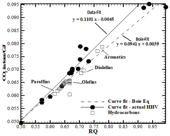
Figure 4.
Variation of CO2 emitted in tons per GJ of energy released (or Giga Tons per Exa J) for fuels with RQ of fuels. Figure adopted from [7]. Measured heating value and composition data were used to estimate the CO2 released in tons per GJ and RQ of fuels. The sloped values are compared with the slope obtained from the use of empirical Boie equation for gross or higher heating value (HHV) kJ/kg of fuel = {35,160 YC + 116225 ∗ YH − 11,090 ∗ YO + 6280 YN + 10,465 YS, where YC, YH, YN, YO, and YS are mass fractions of carbon, hydrogen, nitrogen, oxygen, and sulfur in a C-H-N-O-S fuel. The slopes of both trend lines were approximately 0.1.
Since C in tons = CO2 in tons ∗ 12.01/44.01 = 0.27 ∗ CO2 in tons, then Equations (8) and (9) become:
It is seen that for coals dominated by C atoms (Table 1), RQ ≈ 1, and hence CO2 in GT per Exa J = 0.1 (or 0.116 short tons per MMBtu), while for CH4 (or natural gas), it is only 0.05 Giga Tons per Exa J.
The higher the RQ values of FF fuels, the more CO2 or C in Giga Tons per Exa J of energy is released. On the other hand, if CO2 in Giga Tons per Exa J is known for a mix of fossil fuels (natural gas, fuel oil, coal, etc.), then the RQ of the mix can be determined (See Section 3.4.1 for more details).
3.3.2. RQ for Incomplete Combustion
The RQ values listed in Table 1 and the CO2 tons per GJ relations in Equations (8)–(11) are best suited for fuels undergoing complete oxidation for applications focused on energy conversion to work. However, RQ’s and Equations (8)–(11) may not be suitable for fuels undergoing moderate to severe incomplete combustion. Consider the release of pure CH4 from cattle feedlots and the incomplete oxidation of flare gas near oil fields and refineries with CO2 and CH4 released into the atm. CH4 is also a global warming gas, but with a CO2eq of around 10.4 (i.e., 10.4 times more potent than CO2 in causing global warming on a mole basis and a 28.5 mass basis called GWP). For these cases, the RQ is estimated by using the following relation:
where [CO2], [O2], and [CH4] are concentrations in ppm. If pure CH4 production in moles/year (=1000 ∗ volume in SCM per year/24.5 or 1.159 ∗ SCF or CH4 mass in g per year/16.05) is known, then
where is volume flow rate in SCM per year
where is volume flow rate in SCF per year. Natural gas flaring is the combustion of natural gas (≈CH4) typically associated with oil extraction. Even though the CH4 flaring has negative environmental effects, the transport of gas is not cost-effective due to a lack of gas pipelines. The average combustion efficiency is 91%, including lit and unlit (3–5%) periods, malfunction, and incomplete combustion [67]. For the gas flares,
where η is the burned or oxidized fraction of CH4.
According to the World Bank’s global gas flaring tracker for 2021, about 140 Giga SCM of natural gas was flared, which releases almost 5 Exa J of energy per year when burned completely. Thus, if 100% is burned, then CO2 emission is 0.25 GT of CO2 (which checks with the relation given by Equation (8) with RQ = 0.5 and energy release = 5 Exa J/year). If 0% is burned, then with a CO2 eq of 10.4, the CO2 eq emission for CH4 is 2.62 GT/year. If 90% is burned and 10% is unburned, then a total of 0.49 GT of CO2/year (=0.25 ∗ 0.9+ 0.1 ∗ 2.62, Equation (19)), which checks with World Bank data, but 0.47 GT of CO2 equivalent is released.
3.3.3. RQ for CO2 Sinks and GT of CO2 Sink per Unit Energy Input
Land and ocean biomasses serve as CO2 sinks and O2 sources. The biomass term is generalized to include terrestrial (land), ocean water, or marine-based biomass and microorganisms. For these CO2 sinks, Equations (8)–(11) can be equally applied, and in this case, they represent the CO2 sink per unit energy input reaching the chlorophyll via PS. Replacing RQ by RQ of growing biomass, RQBM,
It is assumed that the RQBM during growth is the same as the RQBM during the oxidation process; see also Ref. [17], which presumes that the RQBM = 1. If (s) sink data in GT/year are available for biomass, then CO2 in GT/year = 3.667 ∗ C(s) in GT/year and CO2 moles per year = (1/12.01) ∗ (s). The O2 moles produced per year = (1/12.01) ∗ (s)/RQBM. If biomass happens to be C(s) or CH2O(s), RQBM = 1. The ocean RQOWBM has a small spatial variability consistent with previous data [58], and the mean RQOWBM is around 0.7. It is seen in Part II that the RQ of combined land and ocean water-based biomasses is dominated by LBM since net O2 added to atm. is dominated by land-based biomass.
Consider the ocean biomasses, which serves as a CO2 sink. For PP,
- Generic PP: Cx(H2O)w (NH3)yHzH3PO4 or CxH3+2w+3y+z Ny Ow+4 P
Oxidation Reaction: CxH3+2w+3y+z Ny Ow+4 P + {x + (1/4) z} O2→xCO2 +y NH3+ H3PO4 + {w + (½) z}H2O, without nitrification
Nitrification reaction, NH3 + 2O2→ HNO3 + H2O
Overall reaction
CxH3+2w+3y+z Ny Ow+4 P+ {x +2y+ (1/4) z} O2→xCO2 + y HNO3 + H3PO4 +{w +y+ (½) z)}H2O
- (i)
- The ocean plants growth via photosynthesis: (See Table 1) is given by,
106 CO2 + 16 NO3− + H2PO4− + 17 H+ → C106H263O110N16 P + 138 O2,
RQOWBM = {106/138} = 0.77,
- (ii)
- Planktonic marine algae: The Redfield–Ketchum–Richards Formula is given as (CH2O)106(NH3)16 (H3PO4), or C106 H263 O110 N16 P [53] and M = 3553.3 g/mol. Thus, x = 106, y = 16, and w = 106. The RQ is estimated at 0.77. For the RQ based on the traditional Redfield–Ketchum–Richards equation and algae production, see Refs. [43,68].
- (iii)
- Oceanic cyanobacteria and algae: photosynthesis and respiration, RQ = 0.77 [37].
- 2.
- Seaweed or Sargassum: A bright seaweed also absorbs CO2 and produces O2, but it reflects more of the sun’s radiation compared to PP. Using the ultimate analyses reported in [7,69], the chemical formula on the UCF basis is given as CH1.74N0.025O1.42S0.018 (See Table A1, Appendix A.1). Thus, for seaweed, RQBM = 1.57, which is unusually high compared to land-based biomasses. It serves as a good CO2 sink but decomposes and releases NH3 and H2S (odors like rotten eggs) along with CO2. For different seaweeds, Ref. [69] presents ultimate analyses; the author determined the chemical formula and estimated that the RQ of seaweeds could vary from 0.95 to 1.34 (Appendix A.1). The measured RQ values are from 0.99 to 2.38 (or PQ from 0.42 to 1.01), while the theoretical values are from 0.77 to 1 (PQ from 1.0 to 1.3) [70].
3.4. Respiratory Quotient (RQ) of Fossil Fuels and Biomass
3.4.1. RQ of Fossil Fuels (FF)
The RQ can be readily determined for fuels with known chemical formulas. For many solid fuels, ultimate analyses are available (e.g., coal, biomass) and they can be used to derive UCF [7]. When coal, oil, and gas are used as fossil fuels globally, and if % energy delivered is known, then the RQ of this mixture of fuels (RQFF) can be determined. Two methods are suggested for determin0ng RQFF of a mix of FF.
Method I: Use reported data on global CO2 in GT/year and reported annual fossil energy release in Exa J per year [40], then compute GT per Exa J, and use Equation (8) for an estimation of the RQFF.
Method II: Use the RQ values of gas, liquid, and solid fuels (FF) listed in Table 1. RQgas = 0.5 (CH4 or natural gas), RQoil = 0.73 (# 6 Fuel oil low S), RQcoal ≈ 1, estimate their energy fractions (EF) from the global data presented and use the formula RQFF = RQgas ∗ EF gas + RQliq EFoil + RQcoal ∗ EFcoal [7]. Note that the global RQFF will keep changing depending on the energy fractions of coal, gas, and oil.
3.4.2. Respiratory Quotient for the Combined Fossil and Land Use (LU) CO2 (RQFFLU)
In addition to CO2 from FF [71,72,73], land use (LU) (e.g., cutting down forests and burning, soil degradation, fire, clearing lands for agriculture, etc.) also releases CO2. In addition to ref. [21] see also the carbon dioxide information analysis center, for anthropogenic emissions. For the years 2007–2016, LU energy accounted for 13% of anthropogenic CO2 emissions. The land use in 2016 contributed CO2 of 5.6 GT, while the contribution from fossil combustion amounts to 35.4 GT of CO2 [73]. Also see 2020 Special Reports: Land Use, Land-Use Change, and Forestry [74]. The major fraction of CO2 emitted is from FF > 0.8, and the land use energy fraction for CO2 ≤ 0.2. The combination of FF and LU is represented by the acronym FFLU, which includes CO2 contributed by both FF and land use (LU). It is noted that FF is the dominant source of CO2. Thus, the RQ for combined FF and LU is defined as
where NCO₂,FFLU, CO2 released by FFLU, and O2 consumed by FFLU. Thus, the RQ of fossil fuel (RQFF) and the RQ from land use (RQLU) are combined to yield an effective RQFFLU [7]:
where EFk is the energy fraction contributed by fuel k, which same as is ratio of oxygen consumed by fuel k to total oxygen consumed for fuel mix. Ref [7] shows that EFk contributed by fuel k is the same as the ratio of O2 consumed by fuel k to the total O2 consumed by all fuel types due to the constancy of HHVO₂. RQFF = 0.73–0.78 and the land use EFLU ≈ 0.2. For LU, RQLU is set at 1 when estimating RQFFLU.
RQFFLU = RQFF ∗ EFFF + RQLU ∗ EFLU ∗ RQ
3.5. Global Respiratory Quotient (RQGlob) for Planet Earth
The breathing systems within the green planet earth include power plants (NBS, CO2 “exhaled” and air/O2 “inhaled”), humans (BS, CO2 “exhaled” and air/O2 “inhaled”), and biomass on land and in the ocean (BS, CO2 “inhaled” and O2 “exhaled”). As summarized in previous sections, the net CO2 mol added to the atmosphere is the difference between CO2 released by FFLU and the sum of CO2 sinks via biomass and ocean storage, and the O2 mols depleted from the atm is the difference between O2 mols consumed by FFLU and O2 mols produced by biomass. Following the RQ definition used for FF, the global respiratory quotient of planet earth {RQGlob} is defined as
where [d{CO2}/dt]atm (ppm/year, positive) represents the net CO2 added to the atm per year {i.e., the slope of CO2 vs. year} and the net O2 depleted from the atm per year [d{O2}/dt]atm, slope of O2 vs. year in ppm/year, usually negative}. Both slopes can be readily evaluated from linear and quadratic curve fits for Keeling’s data on CO2 and O2 concentration in the atm.
3.6. Data
For presenting the quantitative results on all RQ’s and RQGlob, the following data are required:
- (i).
- Annual fossil and land use energy or annual C or CO2 emission data for FF and LU. Reported data on CO2 are in GT/year and fossil energy consumption in Exa J/year. Data are selected from the carbon dioxide and information analysis center (CDIAC) [71,72,73,74,75]. This method is termed Method I.
- (ii)
- With global energy release data for each fuel type (gas, oil, and coal) and determining the fraction of energy contributed by these three types of FF [76], and the RQ values of gas, oil, and coal (Table 1) and Equation (23), the RQFF can be estimated. This method is termed Method II.
- (iii)
- Respiration Quotient for FF (RQFF) and LU (RQLU), RQLBM, and RQOWBM.
- (iv)
- Curve fit constants for linear and quadratic fits of Keeling’s data on CO2 and O2 vs. years.
See column 3 of Table 2 for a listing of all formulas and a listing of data for quantitative evaluations.
where, , oxygen consumed in Peta moles per year; annual energy consumption by FFLU (Exa J/year). Other necessary data are presented below Table 2 caption.
Table 2.
List of formulas for RQ and other estimations for linear and quadratic curve fits for Keeling’s curves.
For generating numbers for various parameters of interest listed in Table 2, the following data were used:
- (a)
- = 460.21 in 2006 [73]. HHVO2 = 448 kJ/mole of O2 = 0.448 ∗ 10−3 Giga J/mole or 448 Exa J/Peta mole.
- (b)
- For the year 2006, the oxygen consumption rate = 1.027 Peta mols/year with energy per year of 460.21 Exa J/year.
- (c)
- RQFF = 0.75, RQFFLU = 0.775 with energy fraction from LU, EFLU = 0.11; RQLBM, = 1, RQOWBM = 0.87, See also Ref. [77], which quotes PQ = 1.1 or RQLBM = 0.91 for terrestrial plants.
4. Results and Discussion
4.1. RQ of Fossil Fuels (FF)
As outlined in Section 3.4.1, the RQ was determined by two methods:
Method I. Figure 5 shows the results on fossil energy consumed (secondary Y-axis), Peta J/10, CO2 in million tons/year (secondary Y-axis), and RQFF (primary Y-axis) vs. years (Equation (8)). It is seen that CO2 produced by world-wide consumption of gas (RQ = 0.5), oil, and coal (RQ = 1) and energy released from all three sources of FF increased by almost 70%, while the RQFF estimated increases slightly with the years, indicating more use of coal. The average is about 0.75. The RQFF satisfies the inequality 0.5 < RQFF < 1.
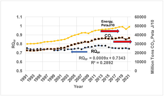
Figure 5.
Variation of world fossil energy consumption in Peta J/10 (secondary axis, 1 Exa J = 1000 Peta J), CO2 emission in million tons (secondary axis), and RQ of FF mix (RQFF, mix of gas, oil, and coal) in power plants (primary axis). “x” in Curve fit = (Year of interest-1991), Year of interest > 1991. The positive slope for RQFF indicates slightly increasing RQ indicating increased use of high RQ Fossil fuels. Note the low R2. The source data for global CO2 from both FF and LU, annual energy consumption by FF (gas, oil, and coal), and energy fractions by each type of FF are taken from Ref. [73]. In 1800, mostly biomass, a renewable fuel, was used. Thus, the only fossil fuel was coal, with RQCoal = 1 around 1800. For PNG and CSV data on FF, see Ref. [78], which also contains Keeling’s curves. Also, this ref. [79] contains world energy data in addition to CO₂ and greenhouse gas emissions. With known CO2 in GT/Exa J = 0.1 ∗ RQ, the RQFF ranges from 0.72 to 0.78 (a linear fit yields 0.73 + 0.0009 ∗ year) with an average of 0.75. Note: for natural gas, which is mostly methane, RQCH4 = 0.5, while RQCoal = 1. Hence, 0.75 indicates RQ of a global average of fossil fuel mixtures of gas, oil, and coal [https://ourworldindata.org/grapher/global-primary-energy, accessed on 18 October 2022]. Ref. [80] states the average CO2 emission from fossil energy from 2010–2019 is 35.2ig ± 1.8 GT CO2/year (9.6 ± 0.5 GT C/year) without the cement carbonation sink and 34.4 ± 1.8 GTt CO2/year (9.4 ± 0.5 GTtC/year) with the cement carbonation sink. With this data, the average FF energy consumption is estimated at 450 Exa J.
Method II. Figure 6 shows a comparison of RQFF estimated using both Methods I and II. As before, RQFF estimated is slightly higher (1991–2009) but almost the same as the RQ from Method I for years beyond 2015.
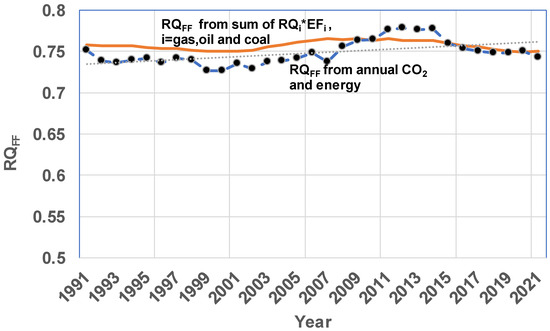
Figure 6.
Comparison on Estimation of RQFF by Method I {reported CO2 and energy data for land fuels used worldwide} with RQFF estimated using Method II {energy contributed and known RQ for each fuel type, {RQgas = 0.5, RQoil = 0.73, RQ Coal = 1}. Data are selected from Ref. [73]. Annual RQFF RQ varies depending on fuel mix used. EF is not shown for all years to reduce clusters of graphs. For 1990: EFgas = 0.235, EFOil = 0.453, EFcoal = 0.312. EF in 2021: EFgas = 0.297, EFOil = 0.376, EFcoal = 0.327. Both Methods I and II yield similar values for RQFF. Keeling presented the ExR (=1/RQ) as 1.4 or RQFF as 0.704–0.714 based on data around 1990 [55,81].
4.2. RQ of FFLU {Combined FF and LU}
C emission data from FF and LU vs. year were collected along with energy released from FF, but land use energy data were not reported. Then, using C emission data for LU and assuming RQLU ≈ 1, the land use energy was estimated by using Equation (8). With known total energy (FF + LU) in Exa J and known CO2 in GT for both FF and LU, RQFFLU vs. year was estimated. Figure 7 shows the results. The RQFFLU average is about 0.78, which is slightly more than the RQFF due to the higher RQ of the land-use fuel source.
4.3. RQ of Land Biomass (RQLBM) and Ocean Water Based Biomass (RQOWBM)
Appendix A.1 lists the ultimate analyses of several biomasses. Using the ultimate analysis, an empirical chemical formula was derived. For many biomass fuels listed in Ref. [82], YC (mass C sink in kg per kg of biomass) varies from 0.346 (rice straw) to 0.5441 (macadamia shells). See Appendix A.1 for the tabulation of RQBM. The RQLBM for land-based dry biomass ranges from 0.94 to 1.05 with an average of 1, which corresponds to a plant with UCF as CH2O or a plant with pure C. It is noted that Huang et al. assumed RQLBM = 1, as though LBM has the chemical formula CH2O [12]. Keeling quotes RQLBM = 0.95, which corresponds to the UCF, CH2O0.4 [55].
CO2(g) + H2O (l) → CH2O (s) + O2 (g), RQLBM = 1

Figure 7.
Comparison of RQ of FF and RQ of RQ combined FF and LU {RQFFLU}. Fossil energy data and fossil and land use C (thus CO2) emission data are from Ref. [73]. Ref. [83] contains world energy data by oil, gas, and coal, 1800–2022. Land use includes CO2 emitted via deforestation and CO2 production via food and wood for construction. Land use CO2 emissions are about 13–20% of total anthropogenic emissions [https://unfccc.int/topics/land-use/workstreams/land-use—land-use-change-and-forestry-lulucf, accessed on 3 November 2023]. Since land use CO2 in GTt/Exa J = 0.1 ∗ RQLU RQ [7] and RQLU ≈ 1 for LU this relation provides an estimate of energy released from land use data.
4.4. Keeling’s Data on CO2 and O2 in ppm and Curve Fits
4.4.1. Keeling’s Data on CO2 and O2
The monthly data file presented by NOAA starting in 1990 was converted into Excel-based data. The calendar period since 1990 was first converted into days in order to capture the zigzag pattern by both CO2 and O2, and O2 concentration in “per meg” units was converted into ppm basis, and the plot of CO2 and O2 vs. days/10 (Figure 8) reveals the zigzag pattern. Looking at the annual history of [CO2 ] and [O2] vs. year, it is clear that the concentration of CO2 starts increasing while that of O2 keeps decreasing from 1990 onwards. An explanation of the zigzag pattern is provided in Section 1 of the Introduction.
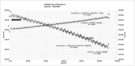
Figure 8.
Keeling’s data on CO2 and O2 and linear and quadratic fits based on data from 1991 to 2021. The Keeling data as Excel file can be accessed at the Scripps-CO2 website [84]; also see Refs. [12,13]. The author converted the dates into days in order to capture saw tooth pattern. Day 1: 19 January 1991. Apart from CO2 released from power plants due to combustion of fuels [13] and CO2 released from warmer oceans in SS, there are CO2 sinks due to biomass growth in SS. For FW period (CO2 ↑, O2 ↓) due to the dominance of CO2 added from power plants compared to CO2 sink via biomass. Hence, there is seasonal “tap dance”: CO2 ↑, O2 ↓ in FW while CO2 ↓, O2 ↑ in SS. Since the increase of CO2 in FW > CO2 sink in SS, the mean for CO2 keeps increasing from year to year while the mean for O2 decreases from year to year. In addition, planet earth is now constantly being charged with other pollutants, such as CH4 with GWP = 10.4 (mole basis), 28.5 (mass basis), N2O with GWP = 273 (mole or mass), and several other trace gases, essentially due to worldwide human activities. AB: straight line fit for CO2, CD: quadratic fit for CO2, EF: straight line fit for O2, GH: quadratic fit for O2. Ppm conversion to GT see ref [85].
4.4.2. The Curve Fits to Keeling’s Data and Estimation of d[CO2]/dt and d[O2]/dt
Two types of curve fits to Keeling data (from 18 April 1991 to 26 January 2021) on [CO2] and [O2] concentrations were obtained.
Linear Fit for CO2 and O2
If the fit is given in terms of (x′ = days/10), say CO2 in ppm = a1 ‘x’+ a0′ then the fit in terms of year is given as CO2 in ppm = a1′ year ∗ (365/10) + a0. Let a1 = a1′ ∗ (365/10), a0′ = a0. Thus, the trend line with a linear fit after conversion from days into years yields:
CO2 in ppm = a1 ∗ years+ a0, a1 = 2.0789, a0 = 350.5 (linear fit), R2 = 0.9709, linear, where years = Year of interest-1991, Year of interest ≥ 1991
In Column 3 of Table 2, the computed numbers for 2006 are given in parentheses in braces { } along with Keeling’s data.
d[CO2]/dt, ppm per year = a1 = 2.0789.
O2 in ppm = b1 ∗ years+ b0, b1 = −4.438 ppm/year, b0 = 209,488 (linear fit), R2 = 0.9839
d[O2]/dt ppm/per year = b1 = −4.438 ppm per year
Column 3 of Table 2 lists the linear curve fit constants along with corresponding derived formulae for several parameters of interest.
HHVO₂ = 448 kJ/mole = 0.448 ∗ 10−3 Giga J/mole or 448 Exa J/Peta mole
4.4.3. Quadratic Fit for CO2 and O2 of Table 2
Since the atm contains air of mass of 5.13 × 1024 g or 1.77 × 10⁶ Peta mol, 1 ppm change of any species by 1 ppm atm = 0.177 Peta mols and, as such, requires a large amount of change of species like CO2 and O2. More fossil fuel use results in more conversion of “carbon” from the ground to CO2, more addition to the atmosphere, and more drop in O2 concentration in the atmosphere, and thus slopes will become steeper in the future. Therefore, a linear fit is not reasonable, and the quadratic fit may reveal such an outcome.
Better accuracy is required, and hence the R2 for the fit must be as high as possible. Thus, a quadratic fit was selected.
where in ppm/year and
where in ppm/year. It is clear that R2 is higher for a quadratic fit.
[CO2] = CO2 in ppm = c2 ∗ years2 + c1 ∗ years + c0, c2 = 0.01892, c1 = 1.473, c0 = 354.1, R2 = 0.9804
[O2] = O2in ppm = d2 ∗ years2 + d1 ∗ years + d0, d2 = −0.04347265, d1 = −3.0332, d0 = 209480, R2 = 0.9896
Column 3 of Table 2 summarizes coefficients fitted curves for both linear and quadratic fits. It also shows the comparison of results between curve fits and actual data. More is the energy consumption, more is the O2 consumption and steeper the slopes of CO2 and O2 curves.
4.5. Estimation of Global Respiration Quotient (RQGlob)
4.5.1. Global RQ Based on CO2 Added to Atm and O2 depleted from Atm
The global respiration coefficient is defined as
where slopes are provided from curve fit constants on Keeling’s curves.
Linear fit: The linear fit indicates that CO2 increases by 2.09 ppm per year while atmospheric oxygen decreases at a rate of 4.438 ppm per year. Using a linear fit for Keeling’s data on CO2 and O2 over 30 years (1991–2021) and Equation (24),
where “years” represents the (Year of interest—1991).
Quadratic Fit: Selecting a quadratic fit,
where in ppm/year. Using Equation (24),
See Column 3 of Table 2, Column 4 where results are tabulated for a quadratic fit. It is clear that RQ changes with the year. Columns 3 and 4 compare the results for linear and quadratic fits.
Figure 9 shows the variation of RQGlob with year based on a quadratic fit; it shows that RQGlob decreases from 0.48 to 0.46 while a linear fit yields a constant value of 0.47. The decrease in RQGlob is attributed to increasing CO2 storage in the ocean. The RQGlob is not a property, while RQFF and RQBM are properties. The RQGlob is somewhat similar to the RQvent in biology. More detailed discussions are presented in the next section.
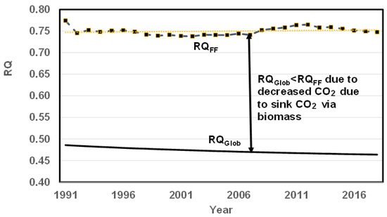
Figure 9.
RQGlob (estimated from quadratic fit) and RQ FF vs. year. There is a slight decrease in RQGlob. The lower the RQGlob, the lower the rate of increase in CO2. RQGlob < RQFFLU mostly due to the storage of CO2 by oceans. Ideally, RQGlob should be zero so that the CO2 concentration in the atm remains constant. Decreasing RQGlob is beneficial for planet earth since it indicates decreasing emissions of CO2, but it is also an indication of increasing CO2 storage in oceans.
4.5.2. RQGlob < RQFFLU and Physical Meaning of RQGlob
The d[CO2]/dt represents the net accumulation of CO2 in atm. It is the difference between CO2 added by FFLU and the sum of CO2 sink by biomass and storage by oceans. Similarly, the magnitude of {d[O2]/dt}atm represents the net depletion rate of O2 in the atm. It is the difference between the O2 used by FFLU and the O2 produced by biomass.
The RQGlob depends on RQFF, RQLBM, RQOWBM, combined Land and ocean water biomass RQLOWBM, annual energy release, CO2 sources, and CO2 sinks. Expanding the relationship for RQGlob,
where , O2 consumed by FFLU, , and O2 produced by both the land and ocean biomasses. Solutions for “x” and “y” are presented in Part II [86]. Since RQ FFLU = 0.78 and RQLOWBM ≈ 1 and approximating RQ FFLU ≈ RQLOWBM,
It is apparent from Equation (30) that the greater the storage of CO2 by the ocean {term: y/(1 − x)}, the lesser is RQGlob < RQFFLU.
As an example, consider the year 2006, for which the annual energy release is known as 460 Exa J/year (which includes FF and LU). With constant HHVO2, the O2 consumed from the atm is given as 1.03 Peta mols/year and with RQFFLU = 0.778, the CO2 released is 1.03 ∗ 0.78 = 0.8 Peta mols/year. The CO2 added to the atm in ppm = 0.8/0.177 = 4.51 ppm since 1 ppm CO2 added to the atm is equivalent to 0.177 Peta mols added to the atm. Similarly, O2 removed from the atm in ppm = 1.03/0.177 = 5.8 ppm. If there were no biomass and no oceans, RQGlob = RQFFLU = 0.778. If the planet has only biomasses, they serve as CO2 sinks and O2 sources. Assuming % CO2 sink by biomass to be 0.32 {Part II}, CO2 sink by biomass = 1.46 ppm, and hence, net CO2 added to the atm = 4.51 − 1.46 = 3.05 ppm. The O2 added by biomass = 1.46 ppm. Thus, net O2 removed from the atm is 5.8 − 1.46 = 4.34 ppm, assuming RQLOWBM ≈ 1. Now RQGlob RQ = 3.05/4.34 = 0.7 and not much change from RQFFLU of 0.778. When ocean CO2 storage of 23% of CO2 from FFLU {Part II} is included, CO2 as stored in the ocean = 0.23 ∗ 4.51 = 1.04 ppm, and hence, net CO2 added to the atm = 3.05 − 1.04 = 2.01 ppm, close to Keeling’s slope: d[CO2]/dt = 2.02 ppm/year/ Now RQGlob = 2.01/4.34 = 0.46 ≈ 0.47< RQFFLU. Hence, the slope {d[CO2[/dt}atm is affected more by the amount of CO2 stored in oceans than by the extent of CO2 sink by biomass. The higher the storage of CO2 by oceans, the lower the RQGlob for given {d[O2]/dt}atm and the higher the acidity of the ocean.
The RQGlob of 0.47 (<RQFFLU = 0.78) is interpreted as the global respiratory quotient of “hypothetical single fossil fuel (HSFF)” releasing 0.47 net moles of CO2 {=CO2 released from combustion of FFLU-CO2 sink via BM and CO2 storage in oceans} for every O2 mole depleted (=O2 consumed by FFLU-O2 produced by LOWBM) from the atmosphere, as though this fictitious power plant is located on a barren earth without ocean water and chlorophyll on the planet. The number 0.47 multiplied by 12.01/44.01 = 0.273 indicates the net amount of moles of C depleted from the reserves of C on the planet. Figure 10 illustrates the difference between the green planet with oceans and the barren planet. Figure 10a represents the earth, with power plants burning FF or FFLU serving as a CO2 source, biomasses undergoing PS with a CO2 sink and O2 source, and oceans serving as CO2 storage. Figure 10b is a fictitious planet somewhat analogous to the metabolism in humans since the “fictitious” barren earth, without chlorophyll and oceans, does not have any mechanism to produce O2 or provide a CO2 sink.
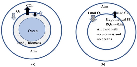
Figure 10.
(a) Planet earth with biomass and oceans. The power plants add CO2 and remove O2 from the atm. PS of BM serves as a sink for a part of CO2 emitted and replenishes the atm partly with O2 produced by BM. (b) Barren planet earth without any biomass or oceans. For this planet, the RQGlob = 0.47. For each mole of O2 depleted from the atm, 0.47 moles of CO2 are added to atm. Hence, 0.47 moles of C or 5.84 kg of C is the mass difference between C of mined FF and the sum of C deposited for the growth of biomass on land and C(s) stored in oceans (which adds weight to land and oceans). Thus, net C(s) leaving land and converted to gaseous CO2 decreases the weight of the earth.
Other consequences of Keeling’s data and RQGlob are as follows: (i) Keeling’s data indicate that the oxygen depletion rate in the atm is 4.48 ppm per year [Magnitude of slope of {d[O2]/dt}atm} and the CO2 addition rate to the atm is 2.082 ppm/year [slope of {d [CO2]/dt}atm}. The normal atmospheric O2 concentration in 1991 was 210,000 ppm. Thus, the depletion rate is extremely small compared to the initial oxygen concentration. However, it is well known that cells of BS do not receive oxygen when the O2 % in atm falls below 16.5 16.5 % or 165,000 ppm [87]. Hence, O2 will reach 165,000 ppm in about 12,000 years with linear fit of O2 data (about 3000 years with quadratic fit) for human extinction or be depleted completely in about 47,000 {=210,000/4.48} years. (ii) The RQGlob of 0.47 indicates that 0.47 net moles of C were removed from the earth {C mined-C stored by ocean water-C removed biomass} and added to the atm as gaseous CO2 per mole of O2 depleted from the atm. Keeling’s data indicate that with 4.3 ppm/year (Column 3 of Table 2) or 0.76 Peta mols of O2/year, the annual loss of C(s) from earth is estimated as 4.3 GT, which presumes that (i) FF can be represented by C-H-O and no sequestration of CO2. Alternately Keeling’s data with linear fit indicates CO2 gain tin atm to be 2.08 ppm or Carbon converted into gas as 2.08 ∗ 0.177 ∗ 12.01 = 4.4 GT/year (ii) All H in fuel gets converted into H2O, which stays on the land/ocean. The C mass loss after 47000 years is estimated at 202,000 GT, {which includes C from coal, oil, and gas} or a decrease in earth’s mass of 202,000 GT, which is negligible compared to the initial earth’s mass of 5.97 ∗ 1012 GT (iii) With CO2 sequestration, the mass loss rate is almost zero. (iv) For the physiological effects of decreasing O2 concentration, see Ref. [88]. (v) The atmospheric pressure is due to the weight of the air over the unit area. Once oxygen is depleted, the weight of the air column decreases, and hence, the atmospheric pressure will decrease due to the depletion of O2. If CO2 addition is ignored or sequestered using underground storage, the atmospheric pressure decreases to 79,000 Pa with 100% N2 in the atmosphere. (vi) If CO2 is not sequestered and continues to be at the current rate, it increases pressure above 79,000 Pa. Now the atm pressure is by both CO2 and N2, and it is estimated at 89,000 Pa {CO2: 11% of N2: 89%}. If all plants, trees, and PP cease to exist, the oxygen production stops [89] and if humans continue to use power plants, oxygen depletion rate due to FF will be 5.8 ppm per year and planet will run out of oxygen in 36,200 years !
4.5.3. RQGlob and Rationality for RQGlob < RQFF
RQGlob is around 0.48 in 1991 to and it decreases to 0.46 in 2021 when a quadratic fit is used (Figure 11) with an average of 0.47 and the RQGlob is constant at 0.47 with a linear fit.
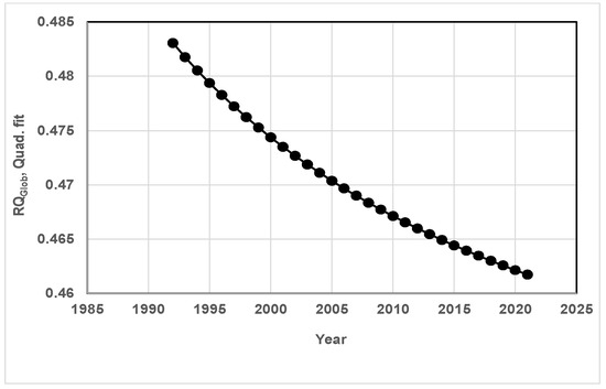
Figure 11.
Variation of RQGlob since 1991 to 2021 for a quadratic fit of Keeling’s data. The RQGlob decreases slightly from 0.48 in 1992 to 0.46 in 2021, revealing increasing acidity of the oceans. Part II of the manuscript indicates similar results. Note that the RQGlob RQ decreases increase in years for a quadratic fit but is constant for a linear fit.
Figure 11 shows decreasing RQGlob with a quadratic fit, revealing increased storage of CO2 in oceans. Furthermore, the increasing ocean surface temperature may release O2 into the atm, thus lowering the RQGlob. [58]. It is seen from Equation (30) that increasing the storage of CO2 in ocean water {term y, Equation (30)} lowers the RQ Glob, which decreases the rate of increase of CO2 in the atm, but at the cost of increasing the acidity of oceans. The website mentioned in Ref. [90] manages “ocean carbon and ocean acidification data”, and the website confirms the increasing acidity of ocean water [91].
Unlike BS, which does not have any mechanism for O2 production within the body, and hence, 0.7< RQ < 1 (without accounting for glycolysis), the breathing planet has a mechanism for O2 production on land and OWBM. Ignoring CO2,st, ocn, the RQGlob is always less than RQFFLU for any x < 1. For a linear fit, the RQGlob is constant at a1/b1 = 0.47, but for a quadratic fit, RQ. Thus, the RQGlob average for 1991–2018 is about 0.47. Ideally, planet earth needs the RQGlob close to zero to maintain CO2 at a constant value.
4.5.4. Predicted Saw-Tooth Pattern of O2 Given CO2 Data and RQGlob
Given the saw-tooth pattern of CO2 data and RQGlob = 0.47, one can predict the O2 pattern RQ (See Appendix A.2 ad Figure A1 for details). Suppose the first data i was on 19 January 1991 (day 1). Then there are a series of readings on several dates: 14 January 1991, 4 April 1991, 18 April 1991 … 18 April 1991 … 30 December 1994. The established O2 in ppm (4 April 91) = O2 in ppm (14 January 91), set at 209,474.2 ppm + {CO2 data in ppm on 4 April 91- CO2 in ppm 14 January 91}/RQGlob, estimated O2 in ppm (18 April 91) = O2 predicted (4 April 91) + {(CO2 data in ppm on 18 April 91) − CO2 in ppm 4 April 91)}/RQGlob, …. Figure 12 shows the saw-tooth pattern for CO2 and O2 (from data) and a comparison of data for O2 with estimated O2 using RQGlob for the period 1991–2020. Since distinction is not clear, Figure 13 shows the blown-up version of the comparison for a short period (1991–1994). It shows data on CO2 and O2 for 1992, 1993, and 1994, predicted O2 (solid line) using RGlob vs. days/10, where days are counted since 19 January 1991. Since the O2 estimate uses CO2 data, the estimated O2 also reveals a saw-tooth pattern. The pattern and prediction of O2 are explained as follows.
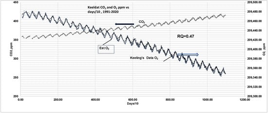
Figure 12.
Comparison of saw-tooth patterns of CO2 and O2 with seasonal uptake of CO2 by biomass in SS and FW. Given the saw-tooth pattern of CO2 data (marker symbols), RQGlob = 0.47, O2 concentrations are predicted as follows: The first data in 1991 were on 19 January 1991 (day 1). Then there are series of readings on 4 April 1991 (75 days from first reading), 18 April 1991 (89 days), 3 May 1991 (104 days), 16 May 1991 (117 days), 30 May 1991 (131 days), so on… Then predicted O2, ppm (day 75) = O2 in ppm (day 1) + {(CO2 in ppm day 75) − CO2 in ppm day 1)}/RQGlob, predicted O2, ppm (day 89) = predicted O2 in ppm (day 75) + {(CO2 in ppm day 89) − CO2 in ppm day 75)}/RQGlob, so on. The predicted saw-tooth pattern for O2 in ppm (solid line) seems to match O2 data (marker symbols) almost exactly for the scale selected. See Figure 13 for a blown-up version.
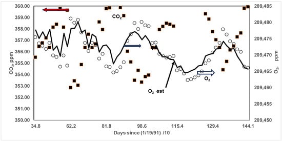
Figure 13.
Magnified view of saw-tooth pattern for years 1991–1994 and comparison of predicted O2. Solid symbols: CO2 data, open symbol: O2 data, solid line: O2 computed using CO2 data and constant RQ = RQSS = RQFW = RQGlob = 0.47 (see Appendix A.2 and Figure A1). The typical amplitude of CO2 is approximately 6 ppm.
The solar input in FW is about 715 kWh/m2 (over 6 months), while the input in SS is about 1130 kWh/m2 (over 6 months), and hence, 57% more for solar input in SS compared to FW. Further, RQSS may be different compared to RQFW., i.e., the BM, a “mixture” of different types of trees and plants in SS and FW {e.g., live oak, which does not shed leaves, vs. post oak, which sheds leaves in FW), may be different in SS and FW, and as such, RQ’s for BM may be different. Further, at the end of FW, the CO2 may also be released by the oxidation of dead leaves by microbes, or the CO2 sink in FW may be less compared to the CO2 sink in SS. The O2 production term due to biomass in Equation (29) for FW < O2 production for SS. There is more depletion of O2 in FW, and hence the slope of {d[O2]/dt} in at FW in FW is also higher. Arguments could be repeated for SS, where CO2 sink increases (numerator term in Equation (29)), lowering CO2 in the atm by BM in SS. But it also increases the O2 production term in the denominator. Thus, compensating effects are present both in SS and FW, so RQGlob may be about the same in both FW and SS {see future work in the manuscript}, as the author assumed. But it is of concern whether the amplitude of variation in CO2 by 6 ppm decreases with more annual energy consumption, which results in a higher release of CO2 but not enough CO2 sink in SS, thus decreasing the amplitude [92]. Keeling’s data are for the northern hemisphere, and the data are not affected by the southern hemisphere (where the seasons are reversed) since the mixing time between the two hemispheres is of the order of one year [92].
4.5.5. Death of BS vs. Death of Green Planet Earth
The BS can live when the RQ (0.7 to 1) and the oxidation reactions deliver the required energy for maintaining life-sustaining functions. However, those reactions involve electron transfer, resulting in the creation of a few radicals that cause damage to cells, thus resulting in the aging of the body and the eventual creation of a birth–death cycle. So, in order to live, the BS must eventually die. A faster oxidation reaction per unit mass of body (i.e., more energy release rate per unit mass, e.g., ants) results in a shorter life span [65]. Green planet earth consists of BS and NBS (e.g., sand, rocks, etc.) that breathe in oxygen and release CO2 with an RQ of 0.47 to support mechanical and leisure life and to live comfortably. In doing so, the terrestrial system undergoes a self-destruction of ecosystems with increasing CO2 in the atm, which results in global warming, the acidity of ocean water, and hence, the slow death of the green planet.
4.5.6. Earth Tilt Angle and Mining and Drilling of Fossil Fuels
The normal tilt angle of the earth is about 23.5 degrees. Earth has been shown to be tilted 80 cm (80 cm or 31.5”) farther east over the last 30 years [93,94]. The tilt is attributed to pumping a large mass of water {2150 GT, 1993–2010 with a total of 17 years, 126 GT/year} from the reservoirs containing 2.0 ∗ 1012 tons of water and a tilt of about 4.4 cm/year due to a shift in water masses. The tilt rate per unit mass of water shift is 0.037cm per GT. Similarly it was shown that mining fossil fuels at locations farther from axis of rotation affects the mass distribution and can result in change in moment of inertia affecting earth’s tilt; i.e., the tilt tangle is affected by pumping or, in general, removing a large amount of solid and liquid masses and converting them to gas and thus affecting mass distribution around the globe [94,95]. If so, then one could speculate that the tilt tangle may also be affected by pumping large amounts of oil and gas and mining coal out of the ground or, in general, removing a large amount of solid and liquid masses and converting them to gas and thus affecting mass distribution around the globe. Unlike the pumping of water, where water undergoes a cyclic process of pumping of water and recovery on land and ocean moderating tilt, the “pumping” of FF converts solids into gas in the atmosphere; as such, the problem of tilt may be more severe! In Section 4.5.2, it was determined that the C mass loss rate from the earth is 4.3 GT/year, and hence, for a period of 17 years, the total mass moved out is 73 GT. Apart from groundwater tilt, it is speculated that there could be an additional tilt of 73 ∗ 0.037 = 2.7 cm over 17 years!
4.5.7. Effects of Presence of CH4 in the Atmosphere
In addition to CO2 and CH4, other global warming gases include H2, N2O, and SF6. The CH4 in the atm increases at a rate of 7.87 ppb/year (not shown) along with CO2 at 2.08 ppm/year or a CO2 total of 2.08 + 10 ∗ 7.87/1000 = 2. 16 ppm/year. Note that the GWP of CH4 is about 10 times that of CO2. O2 typically decreases at a rate of 4.44 ppm/year. Thus
Thus addition of CH4, is equivalent to a total of 17 GT of CO2 added to the atm.
4.5.8. RQGlob and CO2 in Giga Tons per Exa J
When Equation (26) is used in Equations (8) and (9), the relation does not yield GT per Exa J of energy release but yields net GT of CO2/year {i.e., CO2 source—CO2 sink via BM and storage} per Exa J of net energy release {=difference between the energy release from FFLU and energy input via solar energy during PS processes}. When the energy difference is divided by the average heating value of biomasses, it provides the mass of potential FF depleted from planet earth. Part II will introduce fossil energy-based RQGlob,En, which will provide CO2 release per unit Exa J of energy release from FF so that a direct relation between annual FF energy and CO2 in GT per Exa J can be provided.
5. Conclusions
The RQ concept borrowed from biology literature is adopted in engineering literature, and it provides a relation for CO2 in GT per Exa J as 0.1 ∗ RQ and CO2 in million tons per MMBtu as equal to 0.116 ∗ RQ. For biomasses that serve as CO2 sinks and O2 sources, CO2 sink in GT per Exa J energy input for biomass growth = 0.1 ∗ RQ. Instead of RQ, the PS literature uses the following terms: ExR, RR, PQ, and RR which are equal to the inverse of RQ. Keeling’s annual data on CO2 and O2 (1991–2018) are used to obtain the global RQ (RQGlob) as RQGlob = 0.47, which implies that net CO2 moles added to the atm (after accounting for CO2 sink by oceans and biomasses= 0.47 per unit ) net mole of O2 removed from the atmosphere RQ. The power plants on earth use natural gas (RQ = 0.5), oil (RQ = 0.7), and coal (RQ = 1) as FF. Based on CO2 and the energy data, RQFF ≈ 0.78. The global RQ for FF satisfies the inequality 0.5 < RQ < 1. While RQFF or RQBM are properties of fuels and biomasses, RQGlob = is not a property and it depends on CO sink in atm, biomass and oceans. The global RQ is lower than 0.78 since the global RQ is affected by O2 production and CO2 sink in addition to CO2 source and O2 sink by FF, and hence the RQGlob of 0.47 < 0.78. The FF with a lower RQ must be selected and biomass with high RQ is desired in order to reduce CO2 added to the atmosphere. The saw-tooth pattern of O2 is predicted with data on CO2 and the global RQ.
6. Future Work
Future work must include the creation of genetically engineered biomasses with high RQ values greater than >1. The RQ concept, along with CO2 and O2 balance equations, may be used for estimating the CO2 distribution in GTt/year and % distribution of CO2 in the atm, land, and ocean, as well as storage in ocean water. The results must be validated by comparing the RQ-based results with those obtained from detailed computer models developed for CO2 stored in the atm, land, and ocean water (Part II). Knowledge of the RQ for SS and FW is required in order to predict the saw-tooth patterns of CO2 and O2 concentrations. Data are needed for studying the effects of (a) oxygen depletion, (b) CO2 addition, and (c) sequestration on the barometric pressure. Since water pumping seems to affect the earth’s tilt angle [93], similar studies are needed on the effects of mining oil and solid fuels from the ground.
Supplementary Materials
The following supporting information can be downloaded at: https://www.mdpi.com/article/10.3390/en17020299/s1, Supplement on curve fits for Keeling’s data on CO2 and O2.
Funding
The work was carried out simply because of curiosity generated by Keeling’s data and its apparent link to RQ defined in biology. There was no funding for the current research on the RQ method for CO2 distribution. The author wishes to acknowledge the partial support of the research funds from the Paul Pepper Professorship.
Data Availability Statement
Data are contained within the article and supplementary materials.
Acknowledgments
The author wished to acknowledge (i) Saravanan, Head Atm. Science Texas A&M for providing the author with a complimentary copy of his Book on “Climate Demon” Cambridge University Press, 2021) which contained Keeling’s sawtooth curves on CO2 and O2, aroused the curiosity of author and provided the vital link to the RQ concept used in biology and engineering, (ii) Megan Simison of the J. Mike Walker ’66 Department of Mechanical Engineering, Texas A&M University, for the English editing of the manuscript.
Conflicts of Interest
The author declares no conflict of interest.
Nomenclature
| Atm | Atmosphere |
| BS | Biological system GPP: gross prod, total prod |
| CSI,CEng | See Section 3.3.2 on incomplete combustion/Flare |
| (s) | Carbon sink o source rate |
| CH | Carbohydrate |
| CO2 eq | CO2 equivalent |
| DAF | Dry ash free |
| Energy release rate from FFLU | |
| EPICA | European Project for Ice Coring in Antarctica |
| ExR | Exchange ratio = 1/RQ |
| F | Fat |
| FF | Fossil fuel |
| FFLU | Fossil fuel and land use |
| FW | Fall or Autumn (Sep, Oct, Nov) and Winter (Dec, Jan, Feb) |
| GCB | Global Carbon Budget |
| GPP | Gross Primary Production |
| GWP | Global warming potential-CO2 Equivalent |
| Giga J | 109 J = 106 kilo J = 103 Mega J = 10 −6 Peta J = 10−9 Exa J |
| GT | Giga tons, 109 Tons |
| HC | Hydrocarbon |
| HHVO₂ | Higher or gross heating value per Peta Oxygen moles |
| HSFF | Hypothetical Single Fossil Fuel |
| LBM | Land biomass |
| LOWBM | Combined land and ocean water biomasses |
| LU | Land use |
| M | Molecular weight |
| MOM | Marine organic matter |
| Mole rates of CO2, O2 per year | |
| CO2 release rate from FFLU and O2 consumption by FFLU, Peta moles/year | |
| NBS | Non-biological systems |
| NC,nut | Number of C atoms in nutrient |
| NCO₂,BM | number of moles of CO2 used by biomass for growth |
| NO₂,BM | number of moles of O2 from biomass |
| NEP | Net Ecosystem Production |
| NPP | Net Primary Production, = GPP- respiration cost |
| Ocn | Ocean |
| OWBM | Ocean water biomass |
| NOAA | National Oceanic and Atmospheric Administration |
| NPP | Net Primary Product in ecosystem |
| Per meg | 4.76 Per Meg = 1 ppm |
| PP | Phytoplankton |
| Ppb | Parts per billion |
| Ppm | Parts per million or molecules per million molecules 1 ppm in atm = 7.77 GT for CO2, 2.12 GT for C, 1 ppm O2 in atm = 5.65 GT [85] |
| PQ | Photosynthetic quotient {= 1/RQ} |
| PS | Photosynthesis |
| Q | Heat |
| ρ | Density |
| RgQ | Regeneration Quotient (=1/RQ) |
| RQ | Respiratory Quotient, Subscript (i) BM Biomass, (ii) FF: Fossil Fuel (iii) FFLU: FF and land use, (iv) Glob: Global (v) Nut: nutrient, (vi) Vent: Ventilated |
| RR | Redfield ratio = 1/RQ |
| SS | Spring (Mar, Apr, May) and Summer (June, July, Aug) |
| St | Storage |
| UCF | Unit Carbon Formula |
| Volume flow rate | |
| Yk | Mass fraction of element k, g of k/g of mixture |
| z | Ratio of Oxygen moles supplied by ocean biomass to atm to total oxygen moles supplied by both Land and Ocean biomasses |
Appendix A
There are two Appendices, with Appendix A listing RQ of land and a few oceans-based biomasses, and Appendix A.2 describes the method of obtaining saw-tooth patterns of O2 from the data on CO2.
Appendix A.1. Respiration Quotient (RQ) for Land Biomasses and Sea Weeds
Table A1.
Respiration quotient (RQ) and C-Sink (g/g biomass) for Biomasses. YC, Carbon sink in g per g dry ash-free biomass, Boie Est (HHV, kJ/kg) = {35160 YC + 116225 ∗ YH − 11090 ∗ YO + 6280 YN + 10465 YS, where YC, YH, YN, YO, and YS are mass fractions of carbon, hydrogen, nitrogen, oxygen, and Sulphur in a C-H-N-O-S fuel. Table contains measured values of HHV. Min YC (g of C/g biomass): 0.346, Max YC: 0.544 Min RQ (mols CO2 used/mols O2 prod): 0.938, Max RQ: 1.046. Source data: [82,96].
| Name | H/C | N/C | O/C | S/C | O/H | HHV, kJ/g | YC | YH | YN | YO | YS | RQBM |
|---|---|---|---|---|---|---|---|---|---|---|---|---|
| Field crops | ||||||||||||
| Alfalfa seed straw | 1.373 | 0.0183 | 0.654 | 1.602 × 10⁻⁴ | 0.476 | 18.45 | 0.468 | 0.054 | 0.01 | 0.407 | 0.0002 | 0.984 |
| Bean straw | 1.547 | 0.0166 | 0.785 | 8.718 × 10⁻⁵ | 0.507 | 17.46 | 0.430 | 0.0559 | 0.0083 | 0.449 | 0.0001 | 1.006 |
| Corn cobs | 1.499 | 0.0086 | 0.733 | 8.042 × 10⁻⁵ | 0.489 | 18.77 | 0.466 | 0.0587 | 0.0047 | 0.455 | 0.0001 | 0.992 |
| Corn stover | 1.515 | 0.0120 | 0.745 | 8.582 × 10⁻⁵ | 0.492 | 17.65 | 0.437 | 0.0556 | 0.0061 | 0.433 | 0.0001 | 0.994 |
| Cotton stalks | 1.527 | 0.0261 | 0.744 | 1.898 × 10⁻⁴ | 0.487 | 15.83 | 0.395 | 0.0507 | 0.012 | 0.391 | 0.0002 | 0.990 |
| Rice straw (fall) | 1.318 | 0.0144 | 0.657 | 7.173 × 10⁻⁴ | 0.499 | 16.28 | 0.418 | 0.0463 | 0.007 | 0.366 | 0.0008 | 0.998 |
| Rice straw (weathered) | 1.351 | 0.0230 | 0.768 | 1.732 × 10⁻³ | 0.568 | 14.56 | 0.346 | 0.0393 | 0.0093 | 0.354 | 0.0016 | 1.046 |
| Wheat straw | 1.376 | 0.0121 | 0.685 | 9.539 × 10⁻⁴ | 0.497 | 17.51 | 0.432 | 0.05 | 0.0061 | 0.394 | 0.0011 | 0.997 |
| Orchard prunings | ||||||||||||
| Almond prunings | 1.226 | 0.0110 | 0.598 | 7.302 × 10⁻⁵ | 0.488 | 20.01 | 0.513 | 0.0529 | 0.0066 | 0.409 | 0.0001 | 0.993 |
| Black Walnut | 1.390 | 0.0038 | 0.652 | 7.522 × 10⁻⁵ | 0.469 | 19.83 | 0.498 | 0.0582 | 0.0022 | 0.433 | 0.0001 | 0.979 |
| English Walnut | 1.346 | 0.0064 | 0.651 | 7.534 × 10⁻⁵ | 0.484 | 19.63 | 0.497 | 0.0563 | 0.0037 | 0.431 | 0.0001 | 0.989 |
| Vineyard prunings | ||||||||||||
| Cabernet Sauvignon | 1.493 | 0.0153 | 0.707 | 3.216 × 10⁻⁴ | 0.474 | 19.03 | 0.466 | 0.0585 | 0.0083 | 0.439 | 0.0004 | 0.980 |
| Chenin Blanc | 1.459 | 0.0154 | 0.655 | 5.461 × 10⁻⁴ | 0.449 | 19.13 | 0.480 | 0.0589 | 0.0086 | 0.419 | 0.0007 | 0.964 |
| Pinot Noir | 1.468 | 0.0156 | 0.685 | 7.947 × 10⁻⁵ | 0.467 | 19.05 | 0.471 | 0.0582 | 0.0086 | 0.430 | 0.0001 | 0.976 |
| Thompson seedless | 1.449 | 0.0139 | 0.687 | 7.912 × 10⁻⁵ | 0.474 | 19.35 | 0.474 | 0.0577 | 0.0077 | 0.433 | 0.0001 | 0.981 |
| Tokay | 1.449 | 0.0135 | 0.670 | 2.353 × 10⁻⁴ | 0.462 | 19.31 | 0.478 | 0.0582 | 0.0075 | 0.426 | 0.0003 | 0.973 |
| Energy crops | ||||||||||||
| Camaldulensis | 1.425 | 0.0052 | 0.674 | 7.645 × 10⁻⁵ | 0.473 | 19.42 | 0.490 | 0.0587 | 0.003 | 0.440 | 0.0001 | 0.981 |
| Globulus | 1.461 | 0.0069 | 0.688 | 7.775 × 10⁻⁵ | 0.471 | 19.23 | 0.482 | 0.0592 | 0.0039 | 0.442 | 0.0001 | 0.979 |
| Grandis | 1.449 | 0.0027 | 0.701 | 7.751 × 10⁻⁵ | 0.484 | 19.35 | 0.483 | 0.0589 | 0.0015 | 0.451 | 0.0001 | 0.988 |
| Casuarina | 1.426 | 0.0104 | 0.670 | 1.541 × 10⁻⁴ | 0.469 | 19.44 | 0.486 | 0.0583 | 0.0059 | 0.434 | 0.0002 | 0.979 |
| Cattails | 1.452 | 0.0148 | 0.742 | 3.486 × 10⁻⁴ | 0.511 | 17.81 | 0.430 | 0.0525 | 0.0074 | 0.425 | 0.0004 | 1.007 |
| Popular | 1.436 | 0.0083 | 0.677 | 7.732 × 10⁻⁵ | 0.471 | 19.38 | 0.485 | 0.0585 | 0.0047 | 0.437 | 0.0001 | 0.980 |
| Sudan grass | 1.427 | 0.0233 | 0.660 | 6.722 × 10⁻⁴ | 0.462 | 17.39 | 0.446 | 0.0535 | 0.0121 | 0.392 | 0.0008 | 0.973 |
| Forest residue | ||||||||||||
| Black Locust | 1.338 | 0.0096 | 0.620 | 7.384 × 10⁻⁵ | 0.464 | 19.71 | 0.507 | 0.0571 | 0.0057 | 0.419 | 0.0001 | 0.976 |
| Chaparral | 1.288 | 0.0099 | 0.643 | 2.396 × 10⁻⁴ | 0.499 | 18.61 | 0.469 | 0.0508 | 0.0054 | 0.402 | 0.0003 | 0.999 |
| Madrone | 1.476 | 0.0011 | 0.703 | 1.561 × 10⁻⁴ | 0.476 | 19.41 | 0.480 | 0.0596 | 0.0006 | 0.450 | 0.0002 | 0.983 |
| Manzanita | 1.466 | 0.0030 | 0.696 | 1.555 × 10⁻⁴ | 0.475 | 19.3 | 0.482 | 0.0594 | 0.0017 | 0.447 | 0.0002 | 0.982 |
| Ponderosa Pine | 1.446 | 0.0010 | 0.676 | 2.282 × 10⁻⁴ | 0.467 | 20.02 | 0.493 | 0.0599 | 0.0006 | 0.444 | 0.0003 | 0.977 |
| Ten Oak | 1.475 | 0.0022 | 0.693 | 7.835 × 10⁻⁵ | 0.470 | 18.93 | 0.478 | 0.0593 | 0.0012 | 0.441 | 0.0001 | 0.978 |
| Redwood | 1.404 | 0.0008 | 0.636 | 2.219 × 10⁻⁴ | 0.453 | 20.72 | 0.506 | 0.0598 | 0.0005 | 0.429 | 0.0003 | 0.968 |
| White Fur | 1.451 | 0.0009 | 0.686 | 7.645 × 10⁻⁵ | 0.472 | 19.95 | 0.490 | 0.0598 | 0.0005 | 0.448 | 0.0001 | 0.980 |
| Food and fiber processing wastes | ||||||||||||
| Almond hulls | 1.392 | 0.0180 | 0.666 | 8.181 × 10⁻⁵ | 0.478 | 18.22 | 0.458 | 0.0536 | 0.0096 | 0.406 | 0.0001 | 0.985 |
| Almond shells | 1.578 | 0.0221 | 0.705 | 1.666 × 10⁻⁴ | 0.447 | 19.38 | 0.450 | 0.0597 | 0.0116 | 0.423 | 0.0002 | 0.960 |
| Babassu husks | 1.269 | 0.0044 | 0.631 | 2.978 × 10⁻⁴ | 0.497 | 19.92 | 0.503 | 0.0537 | 0.0026 | 0.423 | 0.0004 | 0.998 |
| Sugarcane bagasse | 1.420 | 0.0073 | 0.663 | 8.362 × 10⁻⁵ | 0.467 | 17.33 | 0.448 | 0.0535 | 0.0038 | 0.396 | 0.0001 | 0.977 |
| Coconut fiber dust | 1.194 | 0.0077 | 0.592 | 1.192 × 10⁻³ | 0.495 | 20.05 | 0.503 | 0.0505 | 0.0045 | 0.396 | 0.0016 | 0.996 |
| Cocoa hulls | 1.289 | 0.0530 | 0.515 | 9.321 × 10⁻⁴ | 0.399 | 19.04 | 0.482 | 0.0523 | 0.0298 | 0.331 | 0.0012 | 0.938 |
| Cotton gin trash | 1.580 | 0.0453 | 0.689 | 0 | 0.436 | 16.42 | 0.396 | 0.0526 | 0.0209 | 0.363 | 0 | 0.952 |
| Macadamia shells | 1.091 | 0.0057 | 0.548 | 6.885 × 10⁻⁵ | 0.502 | 21.01 | 0.544 | 0.0499 | 0.0036 | 0.397 | 0.0001 | 1.001 |
| Olive pits | 1.518 | 0.0063 | 0.669 | 1.535 × 10⁻⁴ | 0.441 | 21.39 | 0.488 | 0.0623 | 0.0036 | 0.435 | 0.0002 | 0.957 |
| Peach pits | 1.324 | 0.0052 | 0.554 | 3.534 × 10⁻⁴ | 0.419 | 20.82 | 0.530 | 0.059 | 0.0032 | 0.391 | 0.0005 | 0.949 |
| Peanut hulls | 1.419 | 0.0305 | 0.649 | 9.822 × 10⁻⁴ | 0.457 | 18.64 | 0.458 | 0.0546 | 0.0163 | 0.396 | 0.0012 | 0.970 |
| Pistachio shells | 1.440 | 0.0098 | 0.668 | 7.678 × 10⁻⁵ | 0.464 | 19.26 | 0.488 | 0.0591 | 0.0056 | 0.434 | 0.0001 | 0.974 |
| Rice hulls | 1.248 | 0.0084 | 0.657 | 1.829 × 10⁻⁴ | 0.526 | 16.14 | 0.410 | 0.043 | 0.004 | 0.359 | 0.0002 | 1.017 |
| Walnut shells | 1.359 | 0.0036 | 0.651 | 7.495 × 10⁻⁵ | 0.479 | 20.18 | 0.500 | 0.0571 | 0.0021 | 0.434 | 0.0001 | 0.986 |
| Wheat dust | 1.466 | 0.0630 | 0.638 | 1.720 × 10⁻³ | 0.436 | 16.2 | 0.414 | 0.051 | 0.0304 | 0.352 | 0.0019 | 0.953 |
| Trees | ||||||||||||
| Maple wood (dry) | 1.414 | 0.0042 | 0.619 | 0.000 | 0.438 | 16.2 | 0.506 | 0.0602 | 0.0025 | 0.417 | 0 | 0.958 |
| Mesquite (as rec) | 1.358 | 0.0122 | 0.578 | 2.578 × 10⁻⁴ | 0.426 | 16.7 | 0.436 | 0.0498 | 0.0062 | 0.336 | 0.0003 | 0.952 |
| Junifer (as rec) | 1.370 | 0.0049 | 0.563 | 7.599 × 10⁻⁵ | 0.411 | 19 | 0.493 | 0.0568 | 0.0028 | 0.370 | 0.0001 | 0.943 |
| Sea Weeds [69] | ||||||||||||
| Sargassum tenerrimum | 1.741 | 0.0248 | 1.420 | 1.809 × 10⁻² | 0.816 | - | 0.321 | 0.047 | 0.0093 | 0.607 | 0.0155 | 1.345 |
| Sargassum sp. 1 | 1.593 | 0.0532 | 0.965 | 0.000 | 0.606 | - | 0.403 | 0.054 | 0.025 | 0.518 | 0 | 1.092 |
| Sargassum sp. 2 | 1.777 | 0.0461 | 0.674 | 0.000 | 0.379 | 14.7 | 0.255 | 0.0381 | 0.0137 | - | 0 | 0.903 |
| Sargassum horneri | 1.512 | 0.0161 | 0.647 | 1.355 × 10⁻² | 0.428 | 15.44 | 0.489 | 0.0622 | 0.0092 | 0.422 | 0.0177 | 0.936 |
| Sargassum fluitans Dirty | 1.629 | 0.0460 | 0.725 | 1.442 × 10⁻² | 0.445 | 13.87 | 0.270 | 0.037 | 0.0145 | 0.261 | 0.0104 | 0.944 |
| Sargassum fluitans Wash | 1.523 | 0.0362 | 0.706 | 7.579 × 10⁻³ | 0.464 | 15.27 | 0.391 | 0.05 | 0.0165 | 0.367 | 0.0079 | 0.966 |
| OTHERS | 0.000 | 0.0000 | 0.000 | 0.000 | 0.000 | 0 | 0.000 | 0 | 0 | 0.000 | 0 | 0.000 |
| Pineapple | 1.898 | 0.0171 | 0.799 | 0.000 | 0.421 | 15.27 | 0.401 | 0.064 | 0.008 | 0.427 | 0 | 0.930 |
| Grass | 1.585 | 0.0190 | 0.717 | 8.325 × 10⁻⁴ | 0.452 | 15.27 | 0.450 | 0.06 | 0.01 | 0.430 | 0.001 | 0.963 |
In terms of energy units, the total annual primary biomass production on earth (including food, fiber, etc.) is estimated at 1260 EJ/year [97]. Note that the term biomass includes both land- and water-based. Assuming that the biomass is not in oxidized form, the O2 added to the atm through PS is 2.8 Peta moles, assuming the energy required per mole of O2 is the same as the higher heating value per mole of O2, {HHVO₂} = 448 Exa J/Peta mole of O2 [6,7]. For different sea weeds, ref. [69] presents ultimate analyses; the author determined all of the empirical chemical formulae. Also, Sargassum for Sp 1 and Sp 2 assumes YS = 0; further, for Sp. 2, YO is assumed to be equal to 1-YC-YH-YN
Appendix A.2. Saw Tooth Pattern Using RQGlob

Figure A1.
Schematic of CO2 and O2 vs. days. Data for CO2 are available on days A, B, C, D, and E. O2 vs. Days are generated using CO2 data and RQ for SS and FW. AB, CD: FW, BC, DE: SS, Typically CO2, at C > CO2 at A and O2 at C < O2 at A.
Refer to Figure A1. The relation between oxygen concentration at B in terms of oxygen concentration at A, RQGlob, and CO2 concentrations at A and B is given as follows:
where [ ] concentrations in ppm. Using Equation (A1),
[O2,B ] = [O2,A] − ([CO2,B] − [CO2,A])/RQFW
Similarly, O2 at C is given as
Similarly, O2 at C is given as
[O2,C] = [O2,B] + ([CO2,B] − [CO2,c])/RQSS
[O2,C] = [O2,A] − ([CO2,B] − [CO2,A])/RQFW + ([CO2,B] − [CO2,c]/RQSS
Simplifying and rearranging,
The first term on the right is positive. Furthermore, CO2,C > CO2,A. The second term on the right within { } is positive. Hence [O2,C] < [O2,A] In FW, solar energy input is less for PS, while input energy is higher in SS. Hence, there is rapid biomass growth in SS compared to FW, and as such, the CO2 sink is higher in SS compared to FW. Thus, RQ BM in FW may not be the same as RQSS. RQ for BM is a mixture of RQ’s of various types of plants whose RQ’s may differ.
RQ Glob = CO2 added to atm/O2 depleted from atm
The CO2 sink in FW may be less compared to the CO2 sink in SS, thus increasing CO2 with a higher value for (a1)FW. At the same time, O2 production in FW < O2 production in SS, thus depleting more O2 in FW, and hence |b1|FW is also higher. Arguments could be repeated for SS, where CO2 sink increases, lowering {a1}SS along with a decrease in |b1|SS. i.e., compensating effects are present both in FW and SS, and hence one may assume that RQGlob remains approximately constant.
Assuming RQSS = RQFW= RQGlob, then after simplification, Equation (A4) becomes
where typically [CO2,C] > [CO2,A] − Thus [O2,C] < [O2,A].
References
- Available online: https://www.biologyonline.com/dictionary/life (accessed on 8 September 2022).
- Available online: https://www.cropnutrition.com/nutrient-knowledge/oxygen (accessed on 22 December 2021).
- Available online: https://greencover.com/category/seed-production/ (accessed on 8 November 2022).
- Available online: https://archive.ipcc.ch/ipccreports/sres/land_use/index.php?idp=24 (accessed on 24 October 2023).
- Boden, T.A.; Marland, G.; Andres, R.J. Global, Regional, and National Fossil-Fuel CO2 Emissions. In Carbon Dioxide Information Analysis Center, Oak Ridge National Laboratory; U.S. Department of Energy: Oak Ridge, TN, USA, 2010. [Google Scholar]
- Annamalai, K. Respiratory quotient (RQ), exhaust gas analyses, CO2 Emission and applications in automobile engineering. Adv. Automob. Eng. 2013, 2, 2–4. [Google Scholar] [CrossRef]
- Annamalai, K.; Thanapal, S.; Ranjan, D. Ranking renewable and fossil fuels on global warming potential using respiratory quotient (RQ) Concept. J. Combust. 2018, 2018, 1270708. [Google Scholar] [CrossRef]
- Hansen, J.; Sato, M.; Ruedy, R.; Lacis, A.; Oinas, V. Global warming in the twenty-first century: An alternative scenario. Proc. Natl. Acad. Sci. USA 2000, 97, 9875–9880. [Google Scholar] [CrossRef] [PubMed]
- Crutzen, P.J.; Mosier, A.R.; Smith, K.A.; Winiwarter, W. N2O release from agro-biofuel production negates global warming reduction by replacing fossil fuels. Atmos. Chem. Phys. Discuss. 2007, 7, 11191–11205. [Google Scholar]
- Hotsmark, B. Quantifying the global warming potential of CO2 emissions from wood fuels. Glob. Energy 2015, 7, 195–206. [Google Scholar]
- Nejat, P.; Jomehzadeh, F.; Taheri, M.M.; Gohari, M.; Majid, M.Z.A. A global review of energy consumption, CO2 emissions and policy in the residential sector (with an overview of the top ten CO2 emitting countries). Renew. Sustain. Energy Rev. 2015, 43, 843–862. [Google Scholar] [CrossRef]
- Keeling, C.D.; Piper, S.C.; Bacastow, R.B.; Wahlen, M.; Whorf, T.P.; Heimann, M.; Meijer, H.A. Atmospheric CO2 and 13CO2 Exchange with the Terrestrial Biosphere and Oceans from 1978 to 2000: Observations and Carbon Cycle Implications. In A History of Atmospheric CO2 and Its Effects on Plants, Animals, and Ecosystems; Ecological Studies; Springer: New York, NY, USA, 2005; Volume 177, pp. 83–113. [Google Scholar]
- Saravanan, R. Climate Demon; Cambridge Univ Press: Cambridge, UK, 2021. [Google Scholar]
- Balkanski, Y.; Monfray, P.; Battle, M.; Heimann, M. Ocean primary production derived from satellite data: An evaluation with atmospheric oxygen measurements. Glob. Biogeochem. Cycles 1999, 13, 257–271. [Google Scholar] [CrossRef]
- Available online: https://askdruniverse.wsu.edu/2020/01/10/trees-create-oxygen/ (accessed on 16 October 2022).
- Keeling, R.F. Scripps O2 Program Data; UC San Diego Library Digital Collections: San Diego, CA, USA, 2019. [Google Scholar] [CrossRef]
- Huang, J.; Huang, J.; Liu, X.; Li, C.; Ding, L.; Yu, H. The global oxygen budget and its future projection. Sci. Bull. 2018, 63, 1180. [Google Scholar] [CrossRef]
- Available online: https://scripps.ucsd.edu/news/broken-record-atmospheric-carbon-dioxide-levels-jump-again#:~:text=Scripps%20recorded%20a%20May%20CO,an%20elevation%20of%2013%2C600%20feet (accessed on 14 October 2023).
- Duursma, E.K.; Boission, M.P.R.M. Global oceanic and atmospheric oxygen stability considered in relation to the carbon cycle and to different time scales. Oceanol. Acta 1994, 17, 117–141. [Google Scholar]
- Duffy, K.A.; Schwalm, C.R.; Arcus, V.L.; Koch, G.W.; Liang, L.L.; Schipper, L.A. How close are we to the temperature tipping point of the terrestrial biosphere? Sci. Adv. 2021, 7, 3. [Google Scholar] [CrossRef]
- Available online: https://www.chegg.com/homework-help/questions-and-answers/data-let-s-use-1951-1980-average-global-temperature-14-c-base-temperature-create-new-colum-q34424338 (accessed on 24 October 2023).
- Jouzel, J.; Masson-Delmotte, V. EPICA Dome C Ice Core 800KYr deuterium data and temperature estimates. Pangaea 2007. [Google Scholar] [CrossRef]
- Lüthi, D.; Le Floch, M.; Bereiter, B.; Blunier, T.; Barnola, J.-M.; Siegenthaler, U.; Raynaud, D.; Jouzel, J.; Fischer, H.; Kawamura, K. High-resolution carbon dioxide concentration record 650,000–800,000 years before present. Nature 2008, 453, 379–382. [Google Scholar] [CrossRef] [PubMed]
- Jouzel, J.; Masson-Delmotte, V.; Cattani, O.; Dreyfus, G.; Falourd, S.; Hoffmann, G.; Minster, B.; Nouet, J.; Barnola, J.M.; Chappellaz, J.; et al. Orbital and millennial Antarctic climate variability over the past 800,000 years. Science 2007, 317, 793–797. [Google Scholar] [CrossRef] [PubMed]
- Available online: https://eng.libretexts.org/Bookshelves/Environmental_Engineering_(Sustainability_and_Conservation)/Energy_Conservation_for_Environmental_Protection_(Pisupati) (accessed on 24 October 2023).
- Available online: https://www.saildrone.com/news/hurricane-sam-saildrone-sails-back-into-eye-storm (accessed on 24 October 2023).
- Available online: https://www.nytimes.com/interactive/2023/05/09/magazine/hurricane-saildrone.html?unlocked_article_code=VUzdTI4_2Wkbe3pfTGzCSB6C-YwQ-xsFx00o1N8VWsm9ruYqPH8NHVCHj7epbQZdWW5v_5AfzFD3A-GAeKfNoskNsNxBqdlL8EnPCOqk7lhC3wec5TfyBq0X_-hXbKz4fvsT-B (accessed on 9 May 2023).
- Available online: https://urldefense.com/v3/__https://www.weather.gov/media/slc/ClimateBook/Annual*20Average*20Temperature*20By*20Year.pdf__;JSUlJQ!!KwNVnqRv!EkkZzI7LzrTnM3yjfkgKjKtJtqVJ9HO57RQ3sIC32HeaVd51lXEd0bjoolC_4xrzE98kvNco2hXO6U33z4lgxFAy5A$ (accessed on 10 May 2023).
- Zhu, Q.; Jiang, H.; Liu, J.; Peng, C.; Fang, X.; Yu, S.; Zhou, G.; Wei, X.; Ju, W. Forecasting carbon budget under climate change and CO2 fertilization for subtropical region in China using integrated biosphere simulator (IBIS) model. Pol. J. Ecol. 2011, 59, 3–24. Available online: https://pubs.usgs.gov/publication/70036163 (accessed on 10 May 2023).
- Friedlingstein, P.; O’Sullivan, M.; Jones, M.W.; Andrew, R.M.; Gregor, L.; Hauck, J.; Le Quéré, C.; Luijkx, I.T.; Olsen, A.; Peters, G.P.; et al. Global Carbon Budget 2022. Earth Syst. Sci. Data 2022, 14, 4811–4900. [Google Scholar] [CrossRef]
- Gasser, T.; Crepin, L.; Quilcaille, Y.; Houghton, R.A.; Ciais, P.; Obersteiner, M. Historical CO2 emissions from land use and land cover change and their uncertainty. J. Biogeosci. 2020, 17, 4075–4101. [Google Scholar] [CrossRef]
- Watson, R.T.; Noble, J.R.; Bolin, B.; Ravindranath, N.H.; Verardo, D.J.; Dokken, D.J. (Eds.) Land Use, Land-Use Change and Forestry; IPCC: Geneva, Switzerland; Cambridge University Press: Cambridge, UK, 2000. [Google Scholar]
- Gloege, L.; Yan, M.; Zheng, T.; McKinley, G.A. Improved quantification of ocean carbon uptake by using machine learning to merge global models and pCO2 data. J. Adv. Model. Earth Syst. 2022, 14, e2021MS002620. [Google Scholar] [CrossRef]
- Terhaar, J.; Frölicher, T.L.; Joos, F. Observation-constrained estimates of the global ocean carbon sink from Earth system models. J. Biogeosci. 2022, 19, 4431–4457. [Google Scholar] [CrossRef]
- Li, H.; Ilyina, T.; Loughran, T.; Spring, A.; Pongratz, J. Reconstructions and predictions of the global carbon budget with an emission-driven Earth system model. Earth Syst. Dyn. 2023, 14, 101–119. [Google Scholar] [CrossRef]
- Yakir, D. Large rise in carbon uptake by land plants. Nature 2017, 544, 39–40. [Google Scholar] [CrossRef][Green Version]
- David, K. Expected Limits on the Potential for Carbon Dioxide Removal from Artificial Upwelling. J. Front. Mar. Sci. 2022, 9, 841894. [Google Scholar] [CrossRef]
- Li, C.; Huang, J.; Ding, L.; Liu, X.; Han, D.; Huang, J. Estimation of Oceanic and Land Carbon Sinks Based on the Most Recent Oxygen Budget. Earth’s Fut. 2021, 9, e2021EF002124. [Google Scholar] [CrossRef]
- Matthews, H.D.; Zickfeld, K.; Knutti, R.; Allen, M.R. Focus on cumulative emissions, global carbon budgets and the implications for climate mitigation targets. Environ. Res. Lett. 2018, 13, 010201. [Google Scholar] [CrossRef]
- Available online: https://github.com/openclimatedata/global-carbon-budget/blob/main/data/global-carbon-budget.csv#L2 (accessed on 9 May 2023).
- Available online: https://spacemath.gsfc.nasa.gov/earth/6Page54.pdf (accessed on 9 November 2023).
- Moreno, A.R.; Garcia, C.A.; Larkin, A.A.; Lee, J.A.; Wang, W.L.; Moore, J.K.; Primeau, F.W.; Martiny, A.C. Latitudinal gradient in the respiration quotient and the implications for ocean oxygen availability. Proc. Natl. Acad. Sci. USA 2020, 117, 22866–22872. [Google Scholar] [CrossRef] [PubMed]
- Redfield, A.C.; Ketchum, B.H.; Richards, F.A. The influence of organisms on the composition of seawater. Sea 1963, 2, 26–77. [Google Scholar]
- Silva, C.; Annamalai, K. Entropy Generation and Human Aging: Lifespan Entropy and Effect of Physical Activity Level. J. Entropy 2008, 10, 100–123. [Google Scholar] [CrossRef]
- Annamalai, K.; Puri, I.K.; Jog, M.A. Advanced Thermo-Dynamics Engineering, 2nd ed.; CRC/Taylor and Francis: Boca Raton, FL, USA, 2011. [Google Scholar]
- Al-Saady, N.M.; Blackmore, C.M.; Bennett, E.D. High fat, low carbohydrate, enteral feeding lowers PaCO2 and reduces the period of ventilation in artificially ventilated patients. Intensive Care Med. 1989, 15, 290–295. [Google Scholar] [CrossRef]
- Available online: https://en.wikipedia.org/wiki/Respiratory_quotient (accessed on 11 October 2023).
- Available online: https://www.frontiersin.org/articles/10.3389/fendo.2018.00806/full (accessed on 11 October 2023).
- Available online: https://www.lung.org/lung-health-diseases/lung-disease-lookup/copd/living-with-copd/nutrition (accessed on 11 October 2023).
- Pujia, A.; Mazza, E.; Ferro, Y.; Gazzaruso, C.; Coppola, A.; Doldo, P.; Grembiale, R.D.; Pujia, R.; Romeo, S.; Montalcini, T. Lipid Oxidation Assessed by Indirect Calorimetry Predicts Metabolic Syndrome and Type 2 Diabetes. Front. Endocrinol. 2018, 9, 806. [Google Scholar] [CrossRef]
- Patel, H.; Kerndt, C.C.; Bhardwaj, A. Physiology, Respiratory Quotient; StatPearls Publishing: Treasure Island, FL, USA, 2023. Available online: https://www.ncbi.nlm.nih.gov/books/NBK531494 (accessed on 24 August 2023).
- Available online: https://en.wikipedia.org/wiki/Composition_of_the_human_body (accessed on 19 August 2023).
- Anderson, L.A. On the hydrogen and oxygen content of marine phytoplankton. Deep-Sea Res. 1995, 42, 1675–1680. [Google Scholar] [CrossRef]
- Available online: https://en.wikipedia.org/wiki/Phytoplankton (accessed on 23 August 2023).
- Keeling, R.F. The atmospheric oxygen cycle: The oxygen isotopes of atmospheric CO2 and O2 and the O2/N2 ratio. Rev. Geophys. 1995, 33, 1253–1262. [Google Scholar] [CrossRef]
- Pries, C.H.; Angert, A.; Castanha, C.; Hilman, B.; Torn, M.S. Using respiration quotients to track changing sources of soil respiration seasonally and with experimental warming. Biogeosciences 2020, 17, 3045–3055. [Google Scholar] [CrossRef]
- Robinson, C. Microbial Respiration, the Engine of Ocean Deoxygenation. Front. Mar. Sci. 2019, 5, 533. [Google Scholar] [CrossRef]
- Tanioka, T.; Matsumoto, K. Stability of marine organic matter respiration stoichiometry. Geophys. Res. Lett. 2020, 47, e2019GL085564. [Google Scholar] [CrossRef]
- Riser, S.C.; Johnson, K.S. Net production of oxygen in the subtropical ocean. Nature 2008, 451, 323–325. [Google Scholar] [CrossRef] [PubMed]
- Ríos, A.f.; Fraga Pérez, F.F.; Figueiras, F.G. Chemical composition of phytoplankton and Particulate Organic Matter in the Ría de Vigo (NW Spain). Sci. Mar. 1998, 62, 257–271. [Google Scholar] [CrossRef]
- Available online: https://oceanservice.noaa.gov/facts/exploration.html (accessed on 11 May 2023).
- Available online: https://www.noaa.gov/education/resource-collections/ocean-coasts/ocean-acidification (accessed on 10 October 2023).
- Mann, K.H.; Lazier, J.R.N. Chapter 10: The Oceans oand global Climate Change: Physcal and Bilofical Aspects. In Dynamics of Marine Ecosystems: Biological-Physical Interactions in the Oceans; Blackwell Scientific Publications: Boston, MA, USA, 1991; pp. 390–422. [Google Scholar]
- Martin, M.S.; Vernet, M.; Cape, M.R.; Mesa, E.; Huertas, A.D.; Reigstad, M.; Wassmann, P.; Duarte, C.M. Relationship Between Carbon- and Oxygen-Based Primary Productivity in the Arctic Ocean, Svalbard Archipelago. Front. Mar. Sci. 2019, 6, 468. [Google Scholar] [CrossRef]
- Annamalai, K. Oxygen Deficient (OD) Combustion and Metabolism: Allometric Laws of Organs and Kleiber’s Law from OD Metabolism? Systems 2021, 9, 54. [Google Scholar] [CrossRef]
- Popovic, M. Thermodynamic properties of microorganisms: Determination and analysis of enthalpy, entropy, and Gibbs free energy of biomass, cells and colonies of 32 microorganism species. Heliyon 2019, 5, 6. [Google Scholar] [CrossRef] [PubMed]
- Kort, E.A.; Plant, G.; Brandt, A.R.; Chen, Y.; Fordice, G.; Negron AM, G.; Schwietzke, S.; Smith, M.; And Zavala-Araiza, D. Inefficient and unlit natural gas flares both emit large quantities of methane. Science 2022, 377, 1566–1571. [Google Scholar] [CrossRef]
- Available online: https://chem.libretexts.org/Bookshelves/General_Chemistry/Book%3A_ChemPRIME_(Moore_et_al.)/03%3A_Using_Chemical_Equations_in_Calculations/3.03%3A_The_Limiting_Reagent/3.3.02%3A_Environment-_TSP_Ecological_Stoichiometry_and_Algal_Blooms (accessed on 28 October 2022).
- Sosa Olivier, J.A.; Laines Canepa, J.R.; Guerrero Zarate, D.; González Díaz, A.; Figueiras Jaramillo, D.A.; Osorio García, H.K.; Evia López, B. Bioenergetic valorization of Sargassum fluitans in the Mexican Caribbean: The determination of the calorific value and washing mechanism. Energy 2022, 10, 45–63. [Google Scholar] [CrossRef]
- Rosenberg, G.; Littler, D.S.; Littler, M.M.; Oliveira, E.C. Primary production and photosynthetic quotients of seaweeds from Sao Paulo State, Brazil. Bot. Mar. 1995, 38, 369–377. [Google Scholar] [CrossRef]
- Available online: https://energy.appstate.edu/research/work-areas/cdiac-appstate (accessed on 20 August 2022).
- Available online: https://data.ess-dive.lbl.gov/portals/CDIAC (accessed on 13 May 2023).
- Available online: https://github.com/openclimatedata/global-carbon-budget/blob/main/archive/Global_Carbon_Budget_2019v1.0.xlsx (accessed on 2 May 2023).
- Available online: https://www.ipcc.ch/report/land-use-land-use-change-and-forestry/ (accessed on 13 January 2022).
- Available online: https://cdiac.ess-dive.lbl.gov/ftp/ndp030/global (accessed on 14 January 2023).
- Fossil Fuels ‘Stubbornly’ Dominating Global Energy Despite Surge in Renewables: Energy Institute. Available online: https://www.spglobal.com/commodityinsights/en/market-insights/latest-news/oil/062623-fossil-fuels-stubbornly-dominating-global-energy-despite-surge-in-renewables-energy-institute (accessed on 16 November 2022).
- Severinghaus, J.P. Studies of the Terrestrial O2 and Carbon Cycles in Sand Dune Gases and in Biosphere 2. Ph.D. Thesis, Columbia University, New York, NY, USA, 1995. [Google Scholar]
- Available online: https://ourworldindata.org/grapher/annual-change-fossil-fuels?tab=tabl (accessed on 10 August 2023).
- Available online: https://ourworldindata.org/ (accessed on 18 October 2022).
- Friedlingstein, P.; O’Sullivan, M.; Jones, M.W.; Andrew, R.M.; Hauck, J.; Olsen, A.; Peters, G.P.; Peters, W.; Pongratz, J.; Sitch, S.; et al. Global Carbon Budget 2020. Earth Syst. Sci. Data 2020, 12, 3269–3340. [Google Scholar] [CrossRef]
- Keeling, R.F. Measuring correlations between atmospheric oxygen and carbondioxide mole fractions—A preliminary-study in urban air. J. Atmos. Chem. 1988, 7, 153–176. [Google Scholar] [CrossRef]
- Annamalai, K.; Sweeten, J.M.; Ramalingam, S.C. Estimation of gross heating values of biomass fuels. Trans. ASAE 1987, 30, 1205–1208. [Google Scholar] [CrossRef]
- Available online: https://ourworldindata.org/fossil-fuels#global-fossil-fuel-consumption (accessed on 24 August 2023).
- Available online: https://scrippsco2.ucsd.edu/data/atmospheric_co2/primary_mlo_co2_record.html (accessed on 8 August 2023).
- Ballantyne, A.P.; Alden, C.B.; Miller, J.B.; Tans, P.P.; White, J.W.C. Increase in observed net carbon dioxide uptake by land and oceans during the past 50 years. Nature 2012, 488, 70–72. [Google Scholar] [CrossRef] [PubMed]
- Annamalai, K. Breathing Planet Earth: Global Respiratory Quotient (RQglob) From Keeling’s Data and CO2-Budget among the Atmosphere, Land and Oceans. J. Energies 2023. under review. [Google Scholar]
- Available online: https://www.osha.gov/laws-regs/standardinterpretations/2007-04-02-0 (accessed on 6 November 2023).
- Keeling, R.F.; Powell, F.L.; Shaffer, G.; Robbins, P.A.; Simonson, T.S. Impacts of Changes in Atmospheric O2 on Human Physiology. Is There a Basis for Concern? Front. Physiol. 2021, 12, 571137. [Google Scholar] [CrossRef]
- Silva, M.; Lourenço, L.; Alves, R.D.F.B.; Sousa, L.F.; Almeida, S.E.D.S.; Farnese, F.S. Different ways to die in a changing world: Consequences of climate change for tree species performance and survival through an ecophysiological perspective. Ecol. Evol. 2019, 9, 11979–11999. [Google Scholar] [CrossRef]
- Available online: https://www.ncei.noaa.gov/products/ocean-carbon-acidification-data-system (accessed on 1 November 2023).
- Available online: https://www.epa.gov/climate-indicators/climate-change-indicators-ocean-acidity (accessed on 5 November 2023).
- Available online: https://keelingcurve.ucsd.edu/2013/06/04/why-does-atmospheric-co2-peak-in-may (accessed on 13 October 2023).
- Seo, K.-W.; Ryu, D.; Eom, J.; Jeon, T.; Kim, J.-S.; Youm, K.; Chen, J.; Wilson, C.R. Drift of Earth’s Pole Confirms Groundwater Depletion as a Significant Contributor to Global Sea Level Rise 1993–2010. Geophys. Res. Lett. 2023, 50, e2023GL103509. [Google Scholar] [CrossRef]
- Humans Are Pumping Out So Much Groundwater That It’s Changing Earth’s Tilt. Available online: https://www.space.com/earth-tilt-changed-by-groundwater-pumping (accessed on 8 November 2023).
- Kumar, B. Consequences of Fossil Fuel Extraction on the Climate Change of the Earth. In Proceedings of the AGU Chapman Conference on Complexity and Extreme Events in Geosciences in India, Chapman Conference on Complexity and Extreme Events in Geosciences, National Geographical Research Institute, Hyderabd, India, 15–19 February 2010. [Google Scholar]
- Ebeling, J.M.; Jenkins, B.M. Physical and chemical properties of biomass fuels. Trans. ASAE 1985, 28, 898–902. [Google Scholar] [CrossRef]
- Popp, J.; Lakner, Z.; Harangi-Rákos, M.; Fari, M. The effect of bioenergy expansion: Food, energy, and environment. Renew. Sustain. Energy Rev. 2014, 32, 559–578. [Google Scholar] [CrossRef]
Disclaimer/Publisher’s Note: The statements, opinions and data contained in all publications are solely those of the individual author(s) and contributor(s) and not of MDPI and/or the editor(s). MDPI and/or the editor(s) disclaim responsibility for any injury to people or property resulting from any ideas, methods, instructions or products referred to in the content. |
© 2024 by the author. Licensee MDPI, Basel, Switzerland. This article is an open access article distributed under the terms and conditions of the Creative Commons Attribution (CC BY) license (https://creativecommons.org/licenses/by/4.0/).