
A Snake Optimization Algorithm-Based Power System Inertia Estimation Method Considering the Effects of Transient Frequency and Voltage Changes


Abstract
1. Introduction
2. Inertia Estimation Model and Its Transformation
2.1. Inertia Estimation with Traditional Swing Equations
2.2. Transformed Inertia Estimation Model
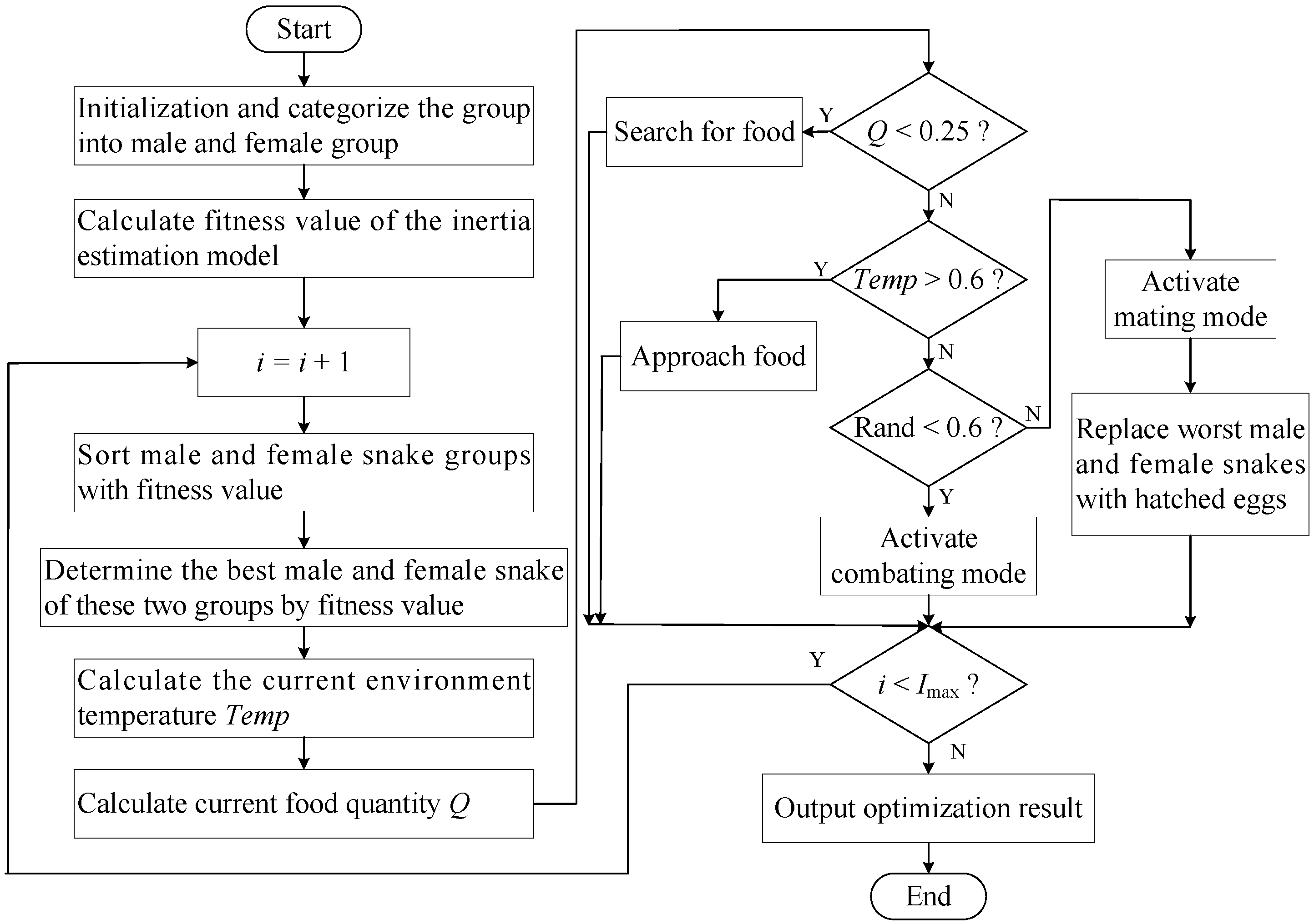
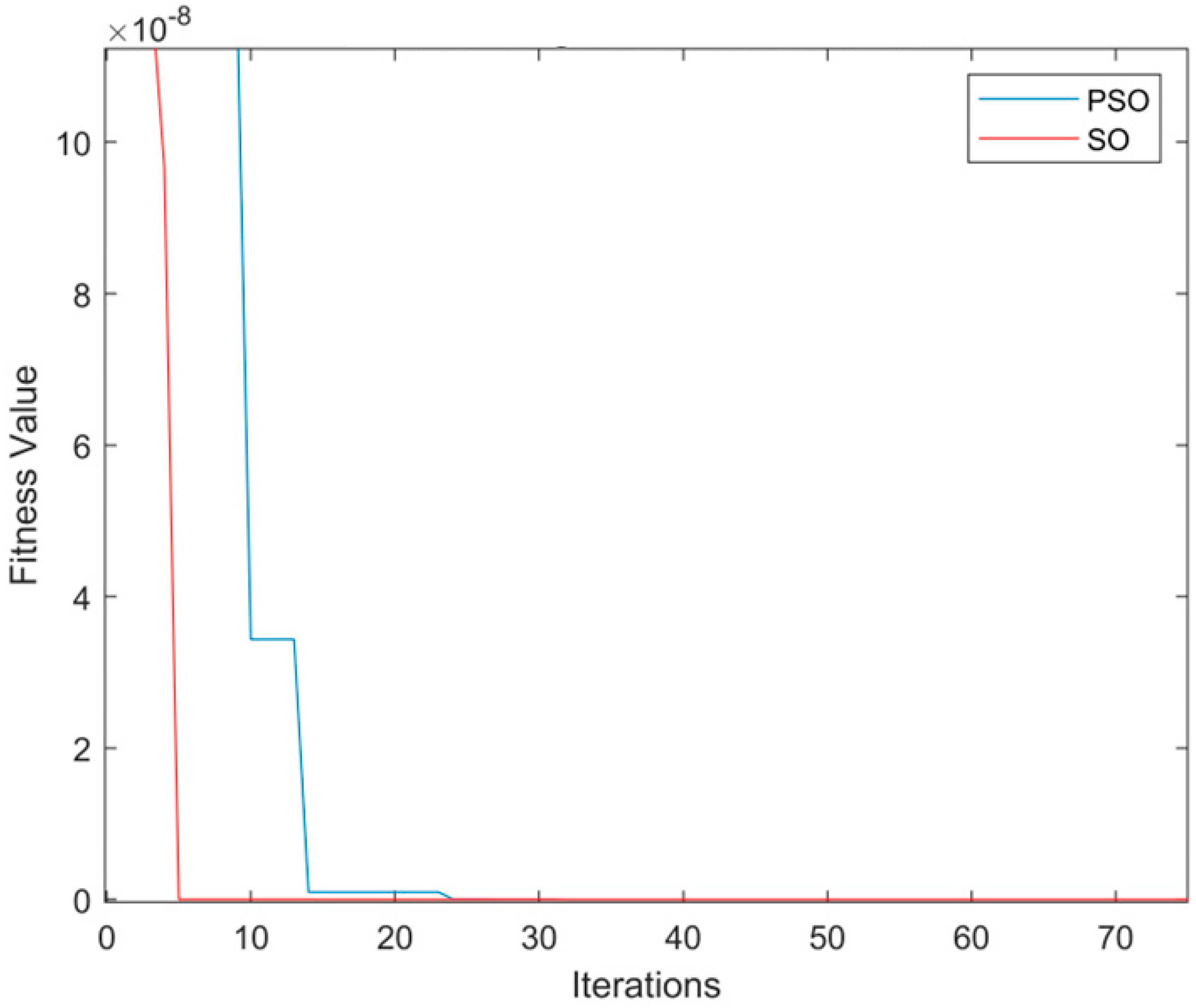
3. Snake Optimization Algorithm-Based Inertia Estimation Method
3.1. Snake Optimization Algorithm
3.1.1. Basics of SO Algorithm
3.1.2. Theoretical Foundation of SO Algorithm
3.2. Application of SO Algorithm in Inertia Estimation
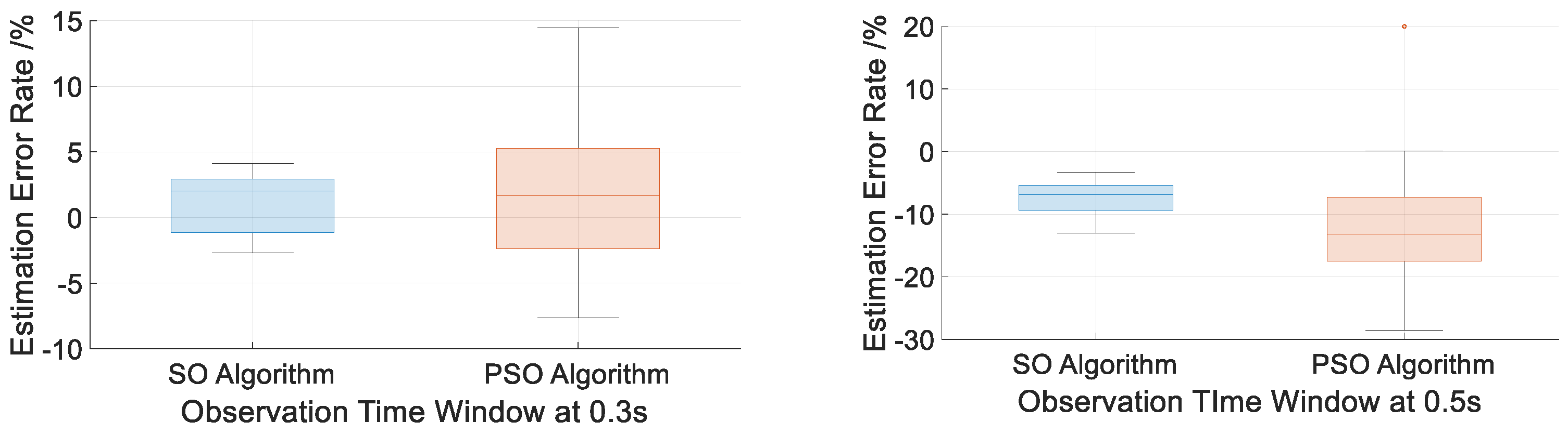
4. Case Study
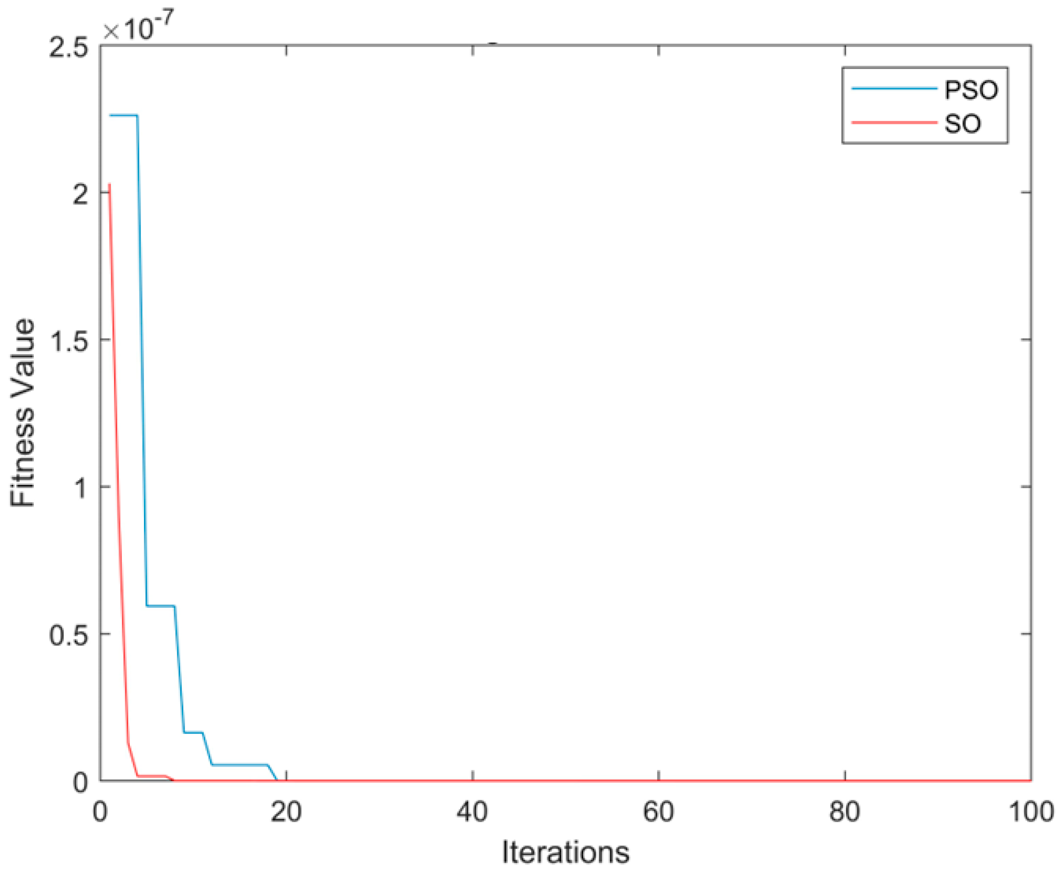
4.1. Test System 1: Two Generators Test System
4.2. Test System 2: Three Generators and Nine Buses Test System
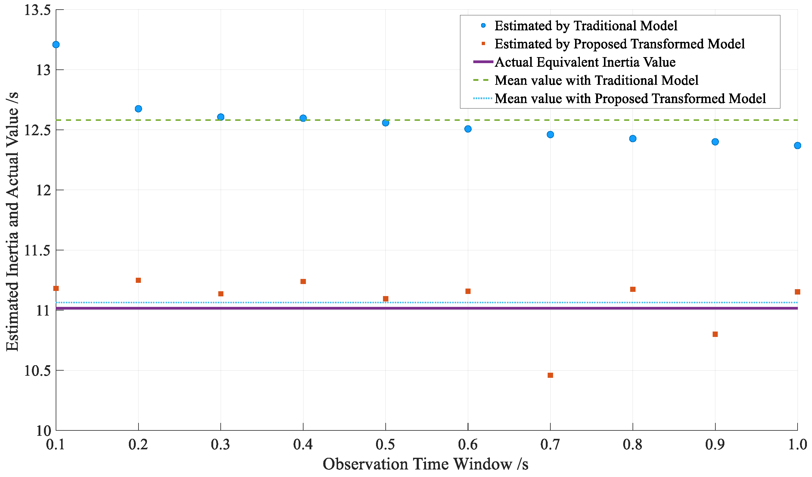
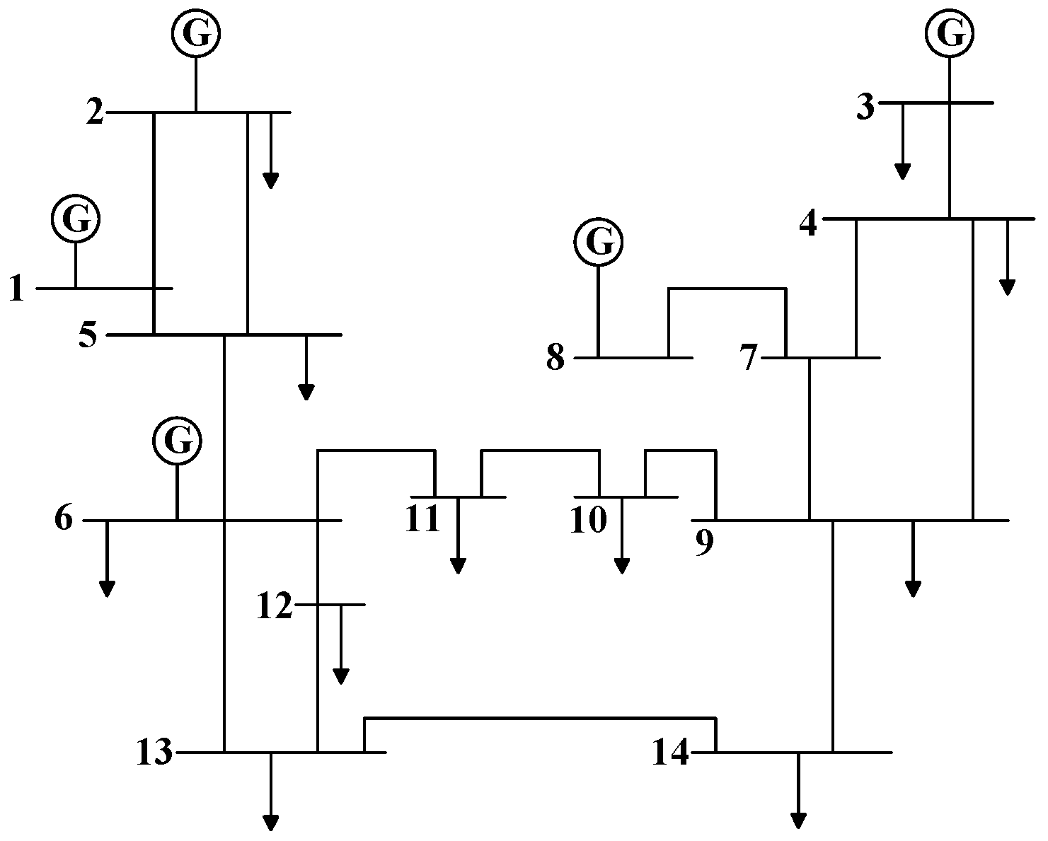
4.3. Test System 3: Five Generators and Fourteen Buses Test System
4.4. Test System 4: Ten Generators and Thirty-Nine Buses Test System
5. Conclusions
Author Contributions
Funding
Data Availability Statement
Conflicts of Interest
References
- Shair, J.; Li, H.; Hu, J.; Xie, X. Power System Stability Issues, Classifications and Research Prospects in the Context of High-Penetration of Renewables and Power Electronics. Renew. Sustain. Energy Rev. 2021, 145, 111111. [Google Scholar] [CrossRef]
- Milano, F.; Dörfler, F.; Hug, G.; Hill, D.J.; Verbič, G. Foundations and Challenges of Low-Inertia Systems. In Proceedings of the 2018 Power Systems Computation Conference (PSCC), Dublin, Ireland, 11–15 June 2018. [Google Scholar]
- National Grid ESO. The Technical Report to the Event of 9 August 2019. Available online: https://www.nationalgrideso.com/document/152346/download (accessed on 1 August 2024).
- Heylen, E.; Teng, F.; Strbac, G. Challenges and Opportunities of Inertia Estimation and Forecasting in Low-Inertia Power Systems. Renew. Sustain. Energy Rev. 2021, 147, 111176. [Google Scholar] [CrossRef]
- Liu, Y.; Sun, M.; Wang, J.; Liao, B.; Wu, J. Inertia Estimation of Nodes and System Based on ARMAX Model. In Proceedings of the 2024 IEEE 2nd International Conference on Power Science and Technology (ICPST), Dali, China, 9–11 May 2024. [Google Scholar]
- Wall, P.; Terzija, V. Simultaneous Estimation of the Time of Disturbance and Inertia in Power Systems. IEEE Trans. Power Deliv. 2014, 29, 2018–2031. [Google Scholar] [CrossRef]
- del Giudice, D.; Grillo, S. Analysis of the Sensitivity of Extended Kalman Filter-Based Inertia Estimation Method to the Assumed Time of Disturbance. Energies 2019, 12, 483. [Google Scholar] [CrossRef]
- Zeng, F.; Zhang, J.; Chen, G.; Wu, Z.; Huang, S.; Liang, Y. Online Estimation of Power System Inertia Constant under Normal Operating Conditions. IEEE Access 2020, 8, 101426–101436. [Google Scholar] [CrossRef]
- Wang, Y.; Yokoyama, A.; Baba, J. A Multifunctional Online Estimation Method for Synchronous Inertia of Power Systems Using Short-Time Phasor Transient Measurement Data with Linear Least Square Method after Disturbance. IEEE Access 2024, 12, 17010–17022. [Google Scholar] [CrossRef]
- Inoue, T.; Taniguchi, H.; Ikeguchi, Y.; Yoshida, K. Estimation of Power System Inertia Constant and Capacity of Spinning-Reserve Support Generators Using Measured Frequency Transients. IEEE Trans. Power Syst. 1997, 12, 136–143. [Google Scholar] [CrossRef]
- Ashton, P.M.; Saunders, C.S.; Taylor, G.A.; Carter, A.M.; Bradley, M.E. Inertia Estimation of the GB Power System Using Synchrophasor Measurements. IEEE Trans. Power Syst. 2015, 30, 701–709. [Google Scholar] [CrossRef]
- Wu, Y.K.; Huang, C.L. Estimation of Power System Inertia- a Case Study in Taiwan. In Proceedings of the 2021 IEEE International Future Energy Electronics Conference (IFEEC), Taipei, China, 16–19 November 2021. [Google Scholar]
- Rodales, D.; Zamora-Mendez, A.; Serna, J.A.D.L.O.; Ramirez, J.M.; Paternina, M.R.A.; Lugnani, L.; Mejia-Ruiz, G.E.; Sanchez-Ocampo, A.; Dotta, D. Model-Free Inertia Estimation in Bulk Power Grids through O-Splines. Int. J. Electr. Power Energy Syst. 2023, 153, 109323. [Google Scholar] [CrossRef]
- Li, D.; Dong, N.; Yao, Y.; Xu, B.; Gao, D.W. Area Inertia Estimation of Power System Containing Wind Power Considering Dispersion of Frequency Response Based on Measured Area Frequency. IET Gener. Transm. Dis. 2022, 16, 4640–4651. [Google Scholar] [CrossRef]
- Cai, G.; Wang, B.; Yang, D.; Sun, Z.; Wang, L. Inertia Estimation Based on Observed Electromechanical Oscillation Response for Power Systems. IEEE Trans. Power Syst. 2019, 34, 4291–4299. [Google Scholar] [CrossRef]
- Panda, R.K.; Mohapatra, A.; Srivastava, S.C. Online Estimation of System Inertia in a Power Network Utilizing Synchrophasor Measurements. IEEE Trans. Power Syst. 2020, 35, 3122–3132. [Google Scholar] [CrossRef]
- Lugnani, L.; Dotta, D.; Lackner, C.; Chow, J. ARMAX-Based Method for Inertial Constant Estimation of Generation Units Using Synchrophasors. Electr. Power Syst. Res. 2020, 180, 106097. [Google Scholar] [CrossRef]
- Kontis, E.O.; Pasiopoulou, I.D.; Kirykos, D.A.; Papadopoulos, T.A.; Papagiannis, G.K. Estimation of Power System Inertia: A Comparative Assessment of Measurement-Based Techniques. Electr. Power Syst. Res. 2021, 196, 107250. [Google Scholar] [CrossRef]
- Azizipanah-Abarghooee, R.; Malekpour, M.; Paolone, M.; Terzija, V. A New Approach to the Online Estimation of the Loss of Generation Size in Power Systems. IEEE Trans. Power Syst. 2019, 34, 2103–2113. [Google Scholar] [CrossRef]
- Wilson, D.; Yu, J.; Al-Ashwal, N.; Heimisson, B.; Terzija, V. Measuring Effective Area Inertia to Determine Fast-Acting Frequency Response Requirements. Int. J. Electr. Power Energy Syst. 2019, 113, 1–8. [Google Scholar] [CrossRef]
- Wang, Y.; Yokoyama, A. An Online Estimation Method of Power System Inertia Using Phasor Measurement Unit Measurements after a Disturbance Considering Damping Effect. In Proceedings of the 2021 IEEE PES Innovative Smart Grid Technologies—Asia (ISGT Asia), Brisbane, Australia, 5–8 December 2021. [Google Scholar]
- Zografos, D.; Ghandhari, M. Power System Inertia Estimation by Approaching Load Power Change after A Disturbance. In Proceedings of the 2017 IEEE Power & Energy Society General Meeting, Chicago, IL, USA, 16–20 July 2017. [Google Scholar]
- Zografos, D.; Ghandhari, M.; Paridari, K. Estimation of Power System Inertia Using Particle Swarm Optimization. In Proceedings of the 2017 19th International Conference on Intelligent System Application to Power Systems (ISAP), San Antonio, TX, USA, 17–20 September 2017. [Google Scholar]
- Hu, P.; Li, Y.; Yu, Y.; Blaabjerg, F. Inertia Estimation of Renewable-Energy-Dominated Power System. Renew. Sustain. Energy Rev. 2023, 183, 113481. [Google Scholar] [CrossRef]
- Hashim, F.A.; Hussien, A.G. Snake Optimizer: A Novel Meta-Heuristic Optimization Algorithm. Knowl.-Based Syst. 2022, 242, 108320. [Google Scholar] [CrossRef]
- Anderson, P.M.; Mirheydar, M. A Low-Order System Frequency Response Model. IEEE Trans. Power Syst. 1990, 5, 720–729. [Google Scholar] [CrossRef]
- IEEE Task Force on Load Representation for Dynamic Performance. Load Representation for Dynamic Performance Analysis (of Power Systems). IEEE Trans. Power Syst. 1993, 8, 472–482. [Google Scholar] [CrossRef]


| Inertia Estimation Model | Unknown Parameters | Range |
|---|---|---|
| Traditional Model | [0, 10] | |
| Proposed Transformed Model | [0, 10] | |
| [0.95, 1.05] | ||
| [1, 2] | ||
| [1, 2] |
| Observation Time Window | Traditional Model | Proposed Transformed Model |
|---|---|---|
| Result/Error | Result/Error | |
| 0.1 s | 7.2464 s/2.2464 s | 5.1636 s/0.1636 s |
| 0.2 s | 6.9042 s/1.9042 s | 5.0737 s/0.0737 s |
| 0.3 s | 6.8231 s/1.8231 s | 4.9727 s/0.0273 s |
| 0.4 s | 6.7889 s/1.7889 s | 4.5924 s/0.4076 s |
| 0.5 s | 6.7502 s/1.7502 s | 4.9574 s/0.0426 s |
| 0.6 s | 6.7024 s/1.7024 s | 4.7194 s/0.2806 s |
| 0.7 s | 6.6636 s/1.6636 s | 5.0877 s/0.0877 s |
| 0.8 s | 6.6485 s/1.6485 s | 5.2210 s/0.2210 s |
| 0.9 s | 6.6540 s/1.6540 s | 4.8786 s/0.1214 s |
| 1.0 s | 6.6628 s/1.6628 s | 5.1089 s/0.1089 s |
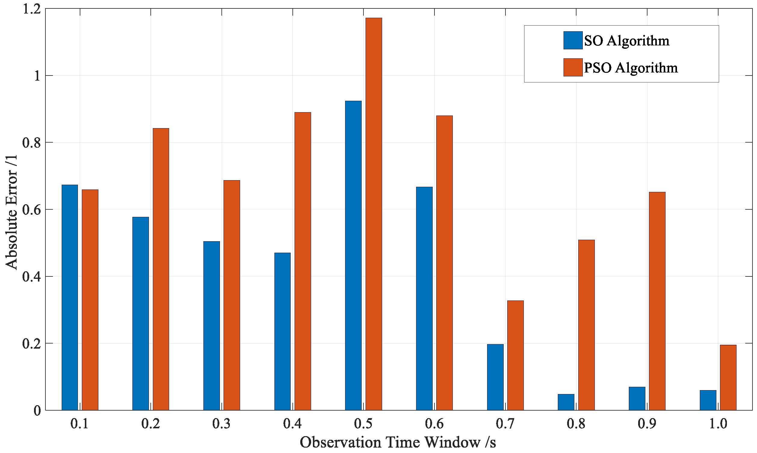
| Observation Time Window | SO Algorithm | PSO Algorithm |
|---|---|---|
| Result/Error | Result/Error | |
| 0.1 s | 11.1811 s/0.1644 s | 11.0044 s/0.0122 s |
| 0.2 s | 11.2491 s/0.2324 s | 10.6033 s/0.4134 s |
| 0.3 s | 11.1360 s/0.1193 s | 10.8402 s/0.1764 s |
| 0.4 s | 11.2394 s/0.2228 s | 10.8879 s/0.1288 s |
| 0.5 s | 11.0946 s/0.0779 s | 10.8111 s/0.2056 s |
| 0.6 s | 11.1578 s/0.1411 s | 10.6317 s/0.3850 s |
| 0.7 s | 10.4590 s/0.5577 s | 10.3673 s/0.6493 s |
| 0.8 s | 11.1742 s/0.1575 s | 10.7420 s/0.2747 s |
| 0.9 s | 10.8005 s/0.2161 s | 10.4266 s/0.5901 s |
| 1.0 s | 11.1524 s/0.1357 s | 10.8906 s/0.1261 s |
| Observation Time Window | Traditional Model | Proposed Transformed Model |
|---|---|---|
| Result/Error | Result/Error | |
| 0.1 s | 95.7974 s/17.5274 s | 90.4395 s/12.1695 s |
| 0.2 s | 91.0843 s/12.8143 s | 81.9380 s/3.6680 s |
| 0.3 s | 90.0319 s/11.7619 s | 80.9137 s/2.6437 s |
| 0.4 s | 90.3709 s/12.1009 s | 77.1445 s/1.1255 s |
| 0.5 s | 91.1961 s/12.9261 s | 69.9666 s/8.3034 s |
| 0.6 s | 92.4855 s/14.2155 s | 71.4888 s/6.7812 s |
| 0.7 s | 93.7382 s/15.4682 s | 70.3299 s/7.9401 s |
| 0.8 s | 95.2051 s/16.9351 s | 72.9294 s/5.3406 s |
| 0.9 s | 96.5379 s/18.2679 s | 71.8028 s/6.4672 s |
| 1.0 s | 97.6417 s/19.3717 s | 67.0750 s/9.1950 s |
Disclaimer/Publisher’s Note: The statements, opinions and data contained in all publications are solely those of the individual author(s) and contributor(s) and not of MDPI and/or the editor(s). MDPI and/or the editor(s) disclaim responsibility for any injury to people or property resulting from any ideas, methods, instructions or products referred to in the content. |
© 2024 by the authors. Licensee MDPI, Basel, Switzerland. This article is an open access article distributed under the terms and conditions of the Creative Commons Attribution (CC BY) license (https://creativecommons.org/licenses/by/4.0/).
Share and Cite
Pang, Y.; Li, F.; Qian, H.; Liu, X.; Yao, Y. A Snake Optimization Algorithm-Based Power System Inertia Estimation Method Considering the Effects of Transient Frequency and Voltage Changes. Energies 2024, 17, 4430. https://doi.org/10.3390/en17174430
Pang Y, Li F, Qian H, Liu X, Yao Y. A Snake Optimization Algorithm-Based Power System Inertia Estimation Method Considering the Effects of Transient Frequency and Voltage Changes. Energies. 2024; 17(17):4430. https://doi.org/10.3390/en17174430
Chicago/Turabian StylePang, Yanzhen, Feng Li, Haiya Qian, Xiaofeng Liu, and Yunting Yao. 2024. "A Snake Optimization Algorithm-Based Power System Inertia Estimation Method Considering the Effects of Transient Frequency and Voltage Changes" Energies 17, no. 17: 4430. https://doi.org/10.3390/en17174430
APA StylePang, Y., Li, F., Qian, H., Liu, X., & Yao, Y. (2024). A Snake Optimization Algorithm-Based Power System Inertia Estimation Method Considering the Effects of Transient Frequency and Voltage Changes. Energies, 17(17), 4430. https://doi.org/10.3390/en17174430