

Resilience Improvement of Microgrid Cluster Systems Based on Two-Stage Robust Optimization


Abstract
1. Introduction
- A DAD model for solving the optimal allocation of ES is proposed, which synergistically optimizes the planning and operation of ES while also considering the uncertainty of damaged lines.
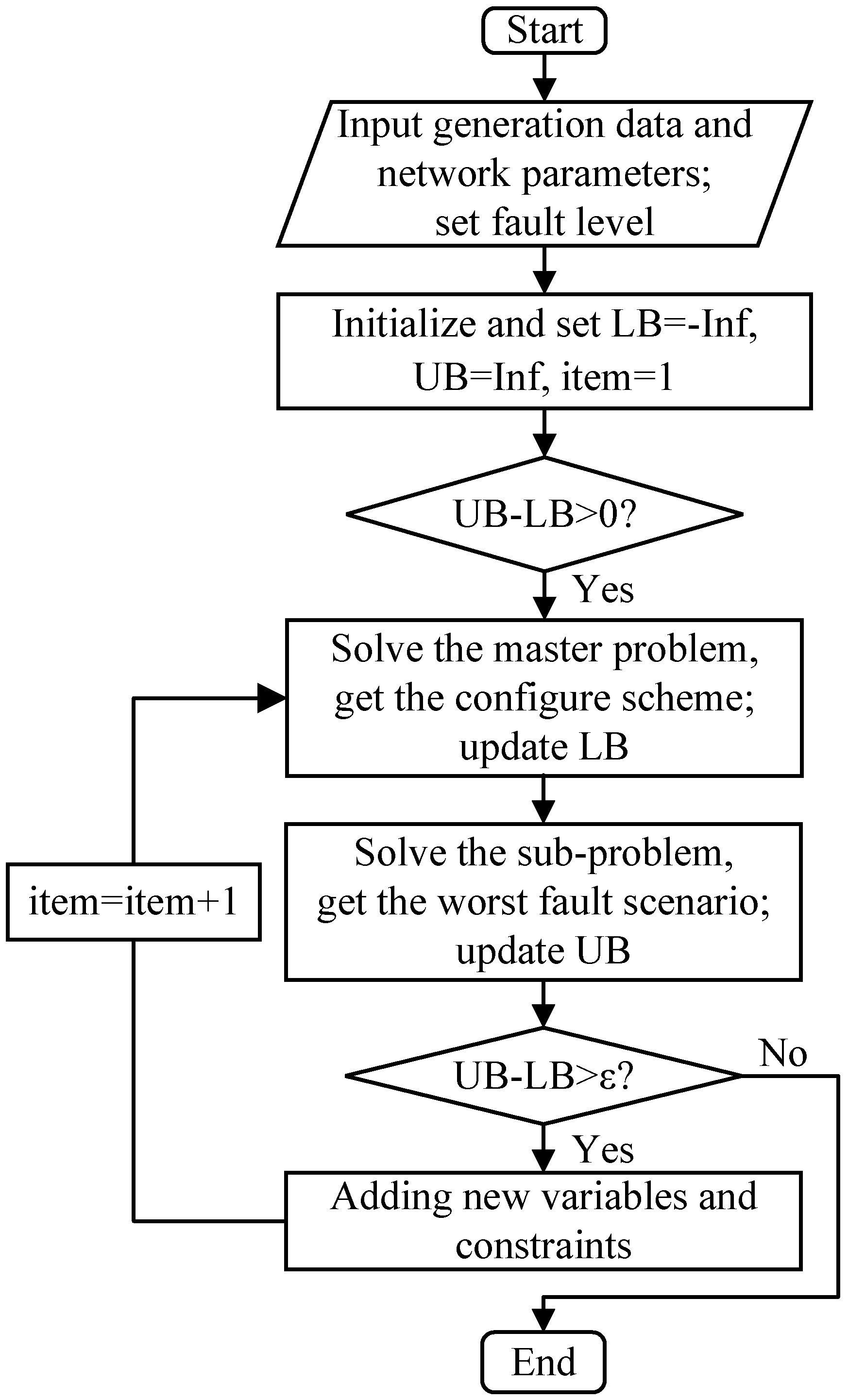
- The column-and-constraint generation (C&CG) algorithm is exploited to solve the problem, with the big-M method for transforming the problem into a mixed integer linear constraint programming problem. The optimal solution can be obtained in a small number of iterations.
2. Formulation of the Problem
2.1. Ocean Power Generation Model
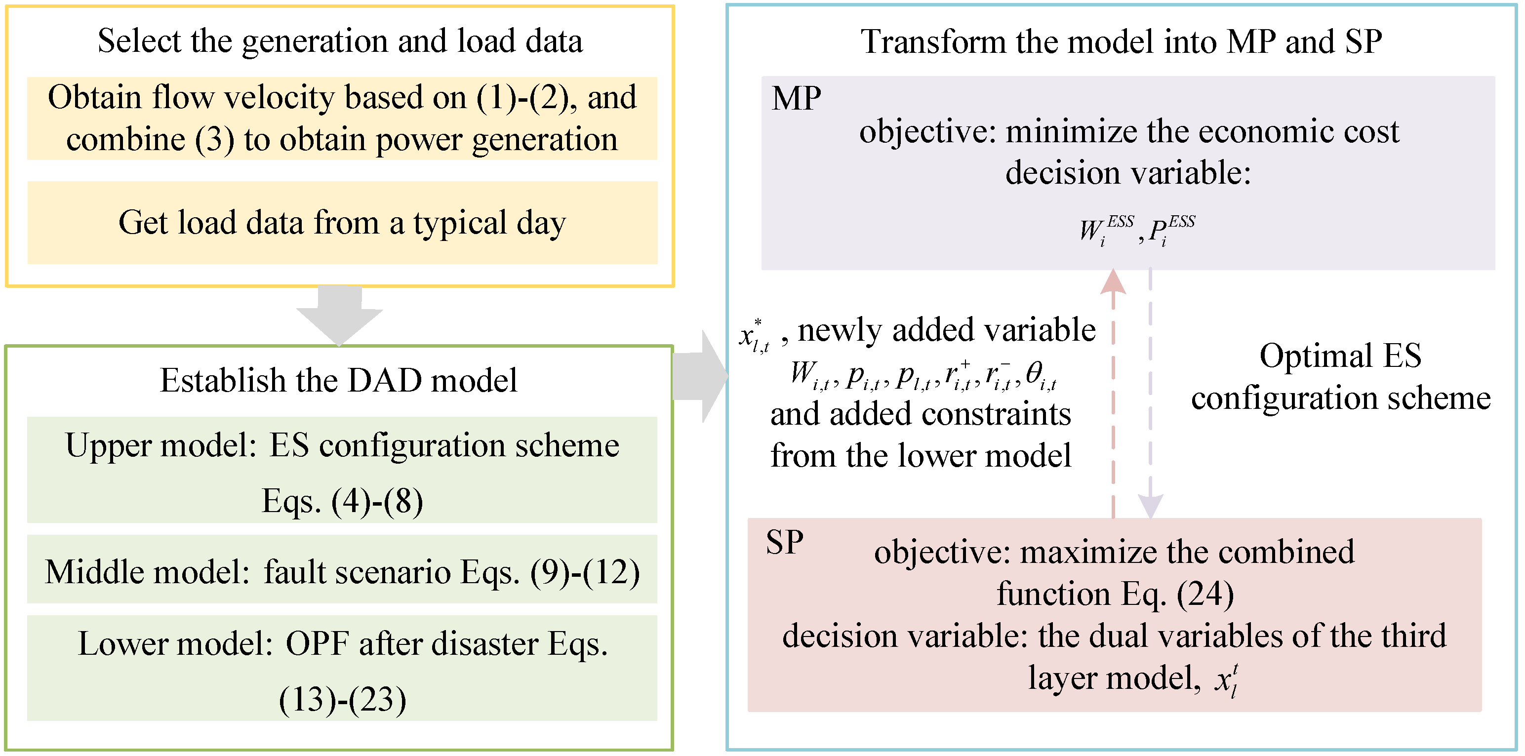
2.2. The DAD Model
3. Solution Method
3.1. The Sub-Problem
3.2. The Master Problem
4. Case Studies
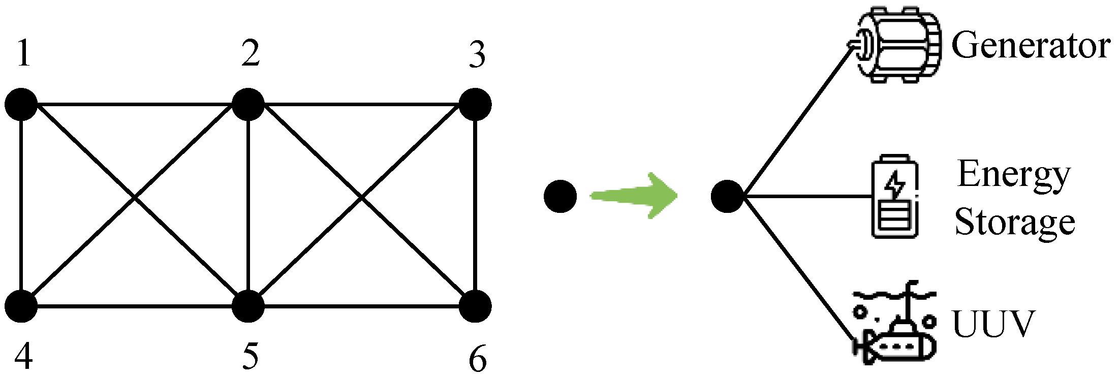
4.1. Six-Bus System
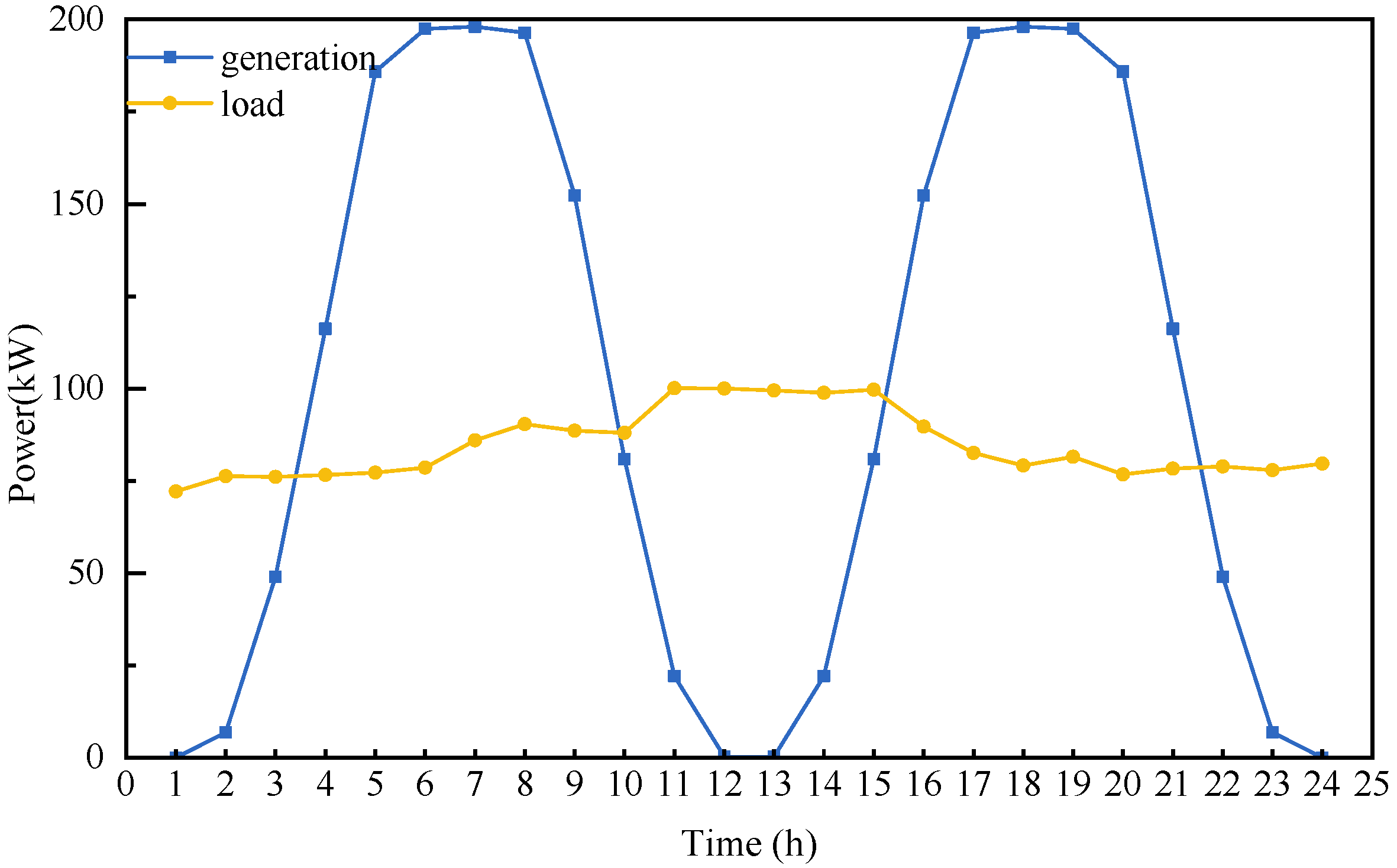
4.1.1. Case Parameters
4.1.2. Configuration Scheme for ES
4.1.3. Comparison before and after ES Configuration
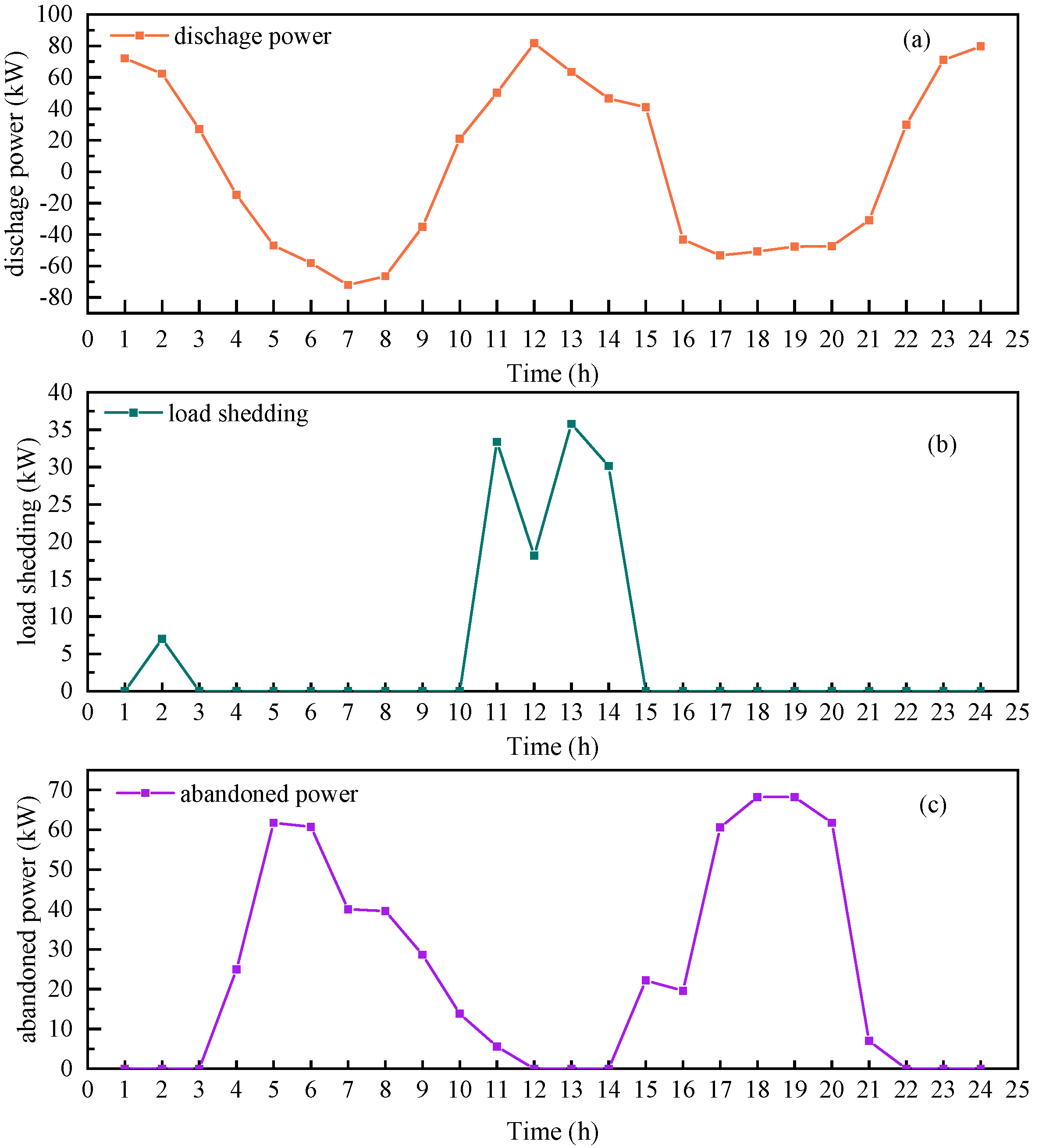
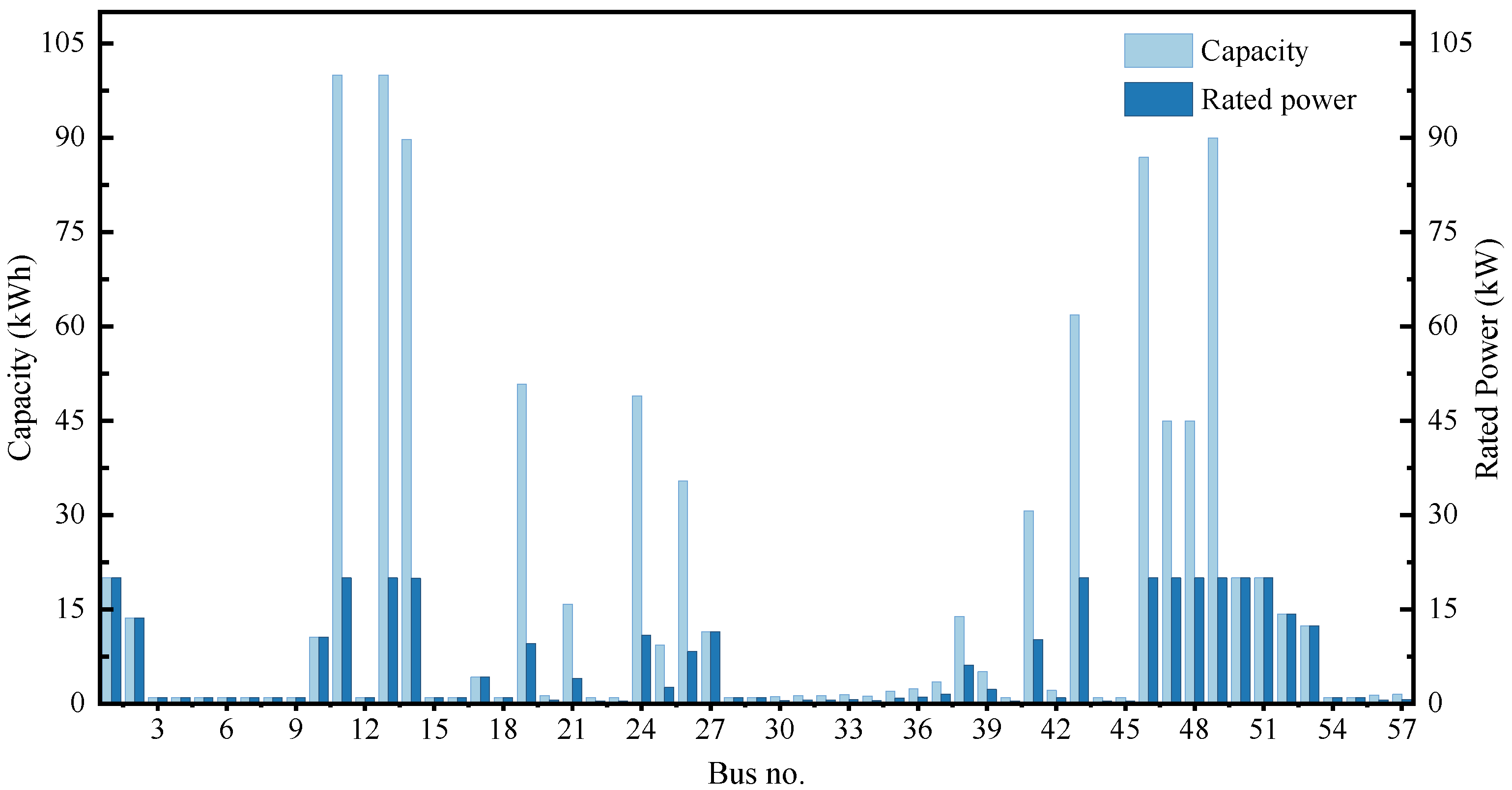
4.2. Fifty-Seven-Bus System
5. Conclusions
Author Contributions
Funding
Data Availability Statement
Conflicts of Interest
Abbreviations
| C&CG | Column-and-Constraint Generation Algorithm |
| DAD | Defender–attacker–defender |
| ES | Energy storage |
| UUV | Unmanned Underwater Vehicle |
Nomenclature
| A. Sets | |
| Set of all buses/transmission lines | |
| T | Set of planning time period |
| B. Parameters | |
| Charging and discharging efficiency of ES | |
| Upper and lower limits of the transmission capacity of line l | |
| a | Rate of inflation |
| b | Discount rate |
| Susceptance of line l | |
| Investment cost per unit capacity of ES | |
| Annual operating cost of unit charging/discharging power for ES | |
| Penalty factor for unit load shed/abandoned power | |
| Power generation and load demand of bus i at time t | |
| k | Upper limit of tripped lines |
| M | Scale factor for the big-M method |
| n | Annual interest rate |
| Total number of buses/lines in the system | |
| Number of generation units located at bus i | |
| Upper and lower limits of rated power for ES configuration | |
| Power output of ocean current power generation units | |
| Period of seawater flow velocity | |
| v | Seawater flow rate |
| Upper and lower limits of ES configuration capacity | |
| y | Lifespan of ES |
| C. Variables | |
| Power angle of bus i at time t | |
| Rated power of ES at bus i | |
| Transmission power of line l at time t | |
| Abandoned power/load shed of bus i at time t | |
| Capacity of ES at bus i | |
| SOC/charging power of ES of bus i at time t | |
| State of line l at time t, with a value of 0 indicating a line fault |
References
- Wang, P.; Chen, L. Economic and Environmental Impacts of Ocean Current Energy Development: A Comparative Analysis. J. Cleaner Prod. 2023, 332, 130106. [Google Scholar]
- Zhou, Z.; Benbouzid, M.; Charpentier, J.F.; Scuiller, F.; Tang, T. A review of energy storage technologies for marine current energy systems. Renew. Sustain. Energy Rev. 2013, 18, 390–400. [Google Scholar] [CrossRef]
- Chen, H.; Tang, T.; Ait-Ahmed, N.; Benbouzid, M.E.H.; Machmoum, M.; Zaim, M.E.H. Attraction, challenge and current status of marine current energy. IEEE Access 2018, 6, 12665–12685. [Google Scholar] [CrossRef]
- Feng, J.C.; Liang, J.; Cai, Y.; Zhang, S.; Xue, J.; Yang, Z. Deep-sea organisms research oriented by deep-sea technologies development. Sci. Bull. 2022, 67, 1802–1816. [Google Scholar] [CrossRef] [PubMed]
- Luo, X.; Wang, J.; Dooner, M.; Clarke, J. Overview of current development in electrical energy storage technologies and the application potential in power system operation. Appl. Energy 2015, 137, 511–536. [Google Scholar] [CrossRef]
- Foteinis, S.; Tsoutsos, T. Strategies to improve sustainability and offset the initial high capital expenditure of wave energy converters (WECs). Renew. Sustain. Energy Rev. 2017, 70, 775–785. [Google Scholar] [CrossRef]
- Nikolaidis, P.; Poullikkas, A. A comparative review of electrical energy storage systems for better sustainability. J. Power Technol. 2017, 97, 220–245. [Google Scholar]
- Cheng, J.; Wang, L.; Pan, T. Optimized Configuration of Distributed Power Generation Based on Multi-Stakeholder and Energy Storage Synergy. IEEE Access 2023, 11, 129773–129787. [Google Scholar] [CrossRef]
- Latio, T.P.B.; Samikannu, R.; Yahya, A.; Karpagam, R.; Kavitha, R.; Deepa, T. Solar Photovoltaic and Battery Storage Systems for Grid-Connected in Urban: A Case study of Juba, South Sudan. In Proceedings of the 2023 IEEE Renewable Energy and Sustainable E-Mobility Conference, Bhopal, India, 17–18 May 2023; pp. 1–7. [Google Scholar]
- Chen, L.; Jiang, Y.; Zheng, S.; Deng, X.; Chen, H.; Islam, M.R. A two-layer optimal configuration approach of energy storage systems for resilience enhancement of active distribution networks. Appl. Energy 2023, 350, 121720. [Google Scholar] [CrossRef]
- Xu, B.; Li, Y.; Wang, Z. Optimal Sizing and Placement of Energy Storage Systems for Marine Renewable Energy Integration. Appl. Energy 2023, 324, 110445. [Google Scholar]
- Chen, H.; Ait-Ahmed, N.; Zaim, E.; Machmoum, M. Marine tidal current systems: State of the art. In Proceedings of the IEEE International Symposium on Industrial Electronics, Bandung, Indonesia, 23–26 September 2012; pp. 1431–1437. [Google Scholar]
- Kuschke, M.; Strunz, K. Modeling of tidal energy conversion systems for smart grid operation. In Proceedings of the IEEE Power and Energy Society General Meeting, Detroit, MI, USA, 24–29 July 2011; pp. 1–3. [Google Scholar]
- Zhang, H.; Ma, S.; Ding, T.; Lin, Y.; Shahidehpour, M. Multi-stage multi-zone defender-attacker-defender model for optimal resilience strategy with distribution line hardening and energy storage system deployment. IEEE Trans. Smart Grid 2020, 12, 1194–1205. [Google Scholar] [CrossRef]
- Hong, S.; Cheng, H.; Zeng, P. N-K constrained composite generation and transmission expansion planning with interval load. IEEE Access 2017, 5, 2779–2789. [Google Scholar] [CrossRef]
- Zeng, B.; Zhao, L. Solving two-stage robust optimization problems using a column-and-constraint generation method. Oper. Res. Lett. 2013, 41, 457–461. [Google Scholar] [CrossRef]
- Geoffrion, A.M. Generalized benders decomposition. J. Optim. Theory Appl. 1972, 10, 237–260. [Google Scholar] [CrossRef]
- Dini, A.; Azarhooshang, A.; Pirouzi, S.; Norouzi, M.; Lehtonen, M. Security-Constrained generation and transmission expansion planning based on optimal bidding in the energy and reserve markets. Electr. Power Syst. Res. 2021, 193, 107017. [Google Scholar] [CrossRef]
- Zimmerman, R.D.; Murillo-Sánchez, C.E.; Thomas, R.J. MATPOWER: Steady-state operations, planning, and analysis tools for power systems research and education. IEEE Trans. Power Syst. 2010, 26, 12–19. [Google Scholar] [CrossRef]
- Anand, R.; Balaji, V. Power flow analysis of simulink IEEE 57 bus test system model using PSAT. Indian J. Sci. Technol. 2015, 8, 1. [Google Scholar] [CrossRef]

| Bus No. | Capacity/kWh | Rated Power/kW |
|---|---|---|
| 1 | 92.2 | 20 |
| 2 | 1 | 0.22 |
| 3 | 100 | 18.10 |
| 4 | 57.44 | 20 |
| 5 | 94.15 | 20 |
| 6 | 61.98 | 13.77 |
| Bus No. | Without ES | With Distributed ES | With Centralized ES | |||
|---|---|---|---|---|---|---|
| Resilience | Abandoned Power Rate | Resilience | Abandoned Power Rate | Resilience | Abandoned Power Rate | |
| 1 | 60.08% | 57.47% | 100% | 27.96% | 60.74% | 42.53% |
| 2 | 67.31% | 52.77% | 100% | 60.08% | 74.59% | 70.69% |
| 3 | 21.52% | 51.42% | 97.43% | 17.24% | 100% | 12.71% |
| 4 | 53.86% | 43.08% | 100% | 31.57% | 100% | 44.36% |
| 5 | 49.81% | 18.15% | 95.10% | 0 | 100% | 18.15% |
| 6 | 53.88% | 57.08% | 100% | 0 | 97.56% | 41.26% |
| Total | 64.14% | 45.93% | 99.16% | 19.72% | 83.39% | 31.27% |
Disclaimer/Publisher’s Note: The statements, opinions and data contained in all publications are solely those of the individual author(s) and contributor(s) and not of MDPI and/or the editor(s). MDPI and/or the editor(s) disclaim responsibility for any injury to people or property resulting from any ideas, methods, instructions or products referred to in the content. |
© 2024 by the authors. Licensee MDPI, Basel, Switzerland. This article is an open access article distributed under the terms and conditions of the Creative Commons Attribution (CC BY) license (https://creativecommons.org/licenses/by/4.0/).
Share and Cite
Ji, S.; Liu, Y.; Wu, S.; Li, X. Resilience Improvement of Microgrid Cluster Systems Based on Two-Stage Robust Optimization. Energies 2024, 17, 4287. https://doi.org/10.3390/en17174287
Ji S, Liu Y, Wu S, Li X. Resilience Improvement of Microgrid Cluster Systems Based on Two-Stage Robust Optimization. Energies. 2024; 17(17):4287. https://doi.org/10.3390/en17174287
Chicago/Turabian StyleJi, Shui, Yun Liu, Shanshan Wu, and Xiao Li. 2024. "Resilience Improvement of Microgrid Cluster Systems Based on Two-Stage Robust Optimization" Energies 17, no. 17: 4287. https://doi.org/10.3390/en17174287
APA StyleJi, S., Liu, Y., Wu, S., & Li, X. (2024). Resilience Improvement of Microgrid Cluster Systems Based on Two-Stage Robust Optimization. Energies, 17(17), 4287. https://doi.org/10.3390/en17174287