Abstract
A modified onboard neuro-fuzzy adaptive (NFA) helicopter turboshaft engine (HTE) automatic control system (ACS) is proposed, which is based on a circuit consisting of a research object, a regulator, an emulator, a compensator, and an observer unit. In this scheme, it is proposed to use the proposed AFNN six-layer hybrid neuro-fuzzy network (NFN) with Sugeno fuzzy inference and a Gaussian membership function for fuzzy variables, which makes it possible to reduce the HTE fuel consumption parameter transient process regulation time by 15.0 times compared with the use of a traditional system automatic control (clear control), 17.5 times compared with the use of a fuzzy ACS (fuzzy control), and 11.25 times compared with the use of a neuro-fuzzy reconfigured ACS based on an ANFIS five-layer hybrid NFN. By applying the Lyapunov method as a criterion, its system stability is proven at any time, with the exception of the initial time, since at the initial time the system is in an equilibrium state. The use of the six-layer ANFF NFN made it possible to reduce the I and II types of error in the HTE fuel consumption controlling task by 1.36…2.06 times compared with the five-layer ANFIS NFN. This work also proposes an AFNN six-layer hybrid NFN training algorithm, which, due to adaptive elements, allows one to change its parameters and settings in real time based on changing conditions or external influences and, as a result, achieve an accuracy of up to 99.98% in the HTE fuel consumption controlling task and reduce losses to 0.2%.
1. Introduction
1.1. Relevance of the Research
Most dynamic systems operate under uncertainty conditions, where there are complex and poorly understood relations between various technological factors, together with the presence of external influences and random interference, as well as nonlinear elements that make the conventional linear adaptive control algorithms difficult to apply [1,2]. In such conditions, the development of effective control strategies becomes a particularly important task. One approach to achieving this task is the hybrid use of neural networks (NNs) [3,4] and fuzzy logic (FL) [5,6]. NNs can train from existing data and identify complex nonlinear relations between the in- and output variables of a system. On the other hand, FL allows us to describe fuzzy or uncertain quantities and relations between them, which makes control models more flexible and adaptive to changing conditions. With the NN and FL hybrid application, the control object and its regulator are described by fuzzy adaptive models. These models can change their structure and parameters during system operation depending on current conditions and control requirements. This approach makes it possible to effectively manage the advanced dynamic systems without requiring precise knowledge of their internal structure or the nature of the influencing external factors [7,8]. The use of hybrid control systems with NNs and FL can lead to significant improvements in the performance and reliability of controlled objects under conditions of environmental uncertainty and variability. Such systems can be successfully used in various fields, including aviation [9,10], industry [11,12], transport [13,14], medicine [15,16], and many others [17,18,19,20].
The relevance of this work lies in addressing the challenges faced by most dynamic systems operating under uncertainty, where complex and poorly understood relationships exist between various technological factors, external influences, and random interference, making conventional linear adaptive control algorithms difficult to apply; the proposed hybrid approach, combining neural networks and fuzzy logic, offers a flexible and adaptive solution for effective management in dynamic environments across various fields.
1.2. State of the Art
Currently, hybrid control integrating NNs and FL is of particular relevance in the gas turbine engine (GTE) controlling context, including HTE. GTEs are complex systems operating under conditions of high dynamics and uncertainty [20,21]. This is where the need arises to develop and apply effective control methods that can adapt to different operating scenarios and ensure high engine performance and reliability. Hybrid control systems, blending the benefits of NNs and FL, provide ample opportunities for fulfilling such tasks [22,23].
For example, in [24], researches employed a fault diagnosis and control system for operations using hybrid multi-mode approaches of the machine learning for monitoring the system health status, using the integration of recurrent feature generation based on NNs and diagnostic modules based on self-organizing maps, including the development of systematic clustering and modeling methodology to create reliable diagnostic modules and check the system efficiency using data from sensors as an example, in relation to the compressor and GTE. A key disadvantage is the limitation of multi-mode and parallel faults, which can pose serious obstacles to the development of reliable diagnostic techniques.
In [25], the authors proposed a model-based learning control method to improve the control quality during the GTE afterburning phase, including offline training and training modules, a power arm angle reference path module, and a built-in nonlinear online inference module, which effectively reduces the total pressure fluctuation on turbine outlet, increases the fan surge margin, and improves thrust linearity. The key disadvantage of this method is its dependence on the accuracy of the model and the possibility of errors due to imperfections in the system model representation.
In [26,27], a modified closed onboard neural network HTE ACS was developed, supplemented with plug-in adaptive control software modules, including a signal adaptation module, a parametric adaptation module, a linear model submodule, and a custom submodule model, differing from current systems, by separating into distinct links for GTE and fuel metering unit (FMU); however, it overlooks the transient processes’ synchronism in the fuel system and the engine itself, which can lead to problems with system overshoot. Overshoot of the developed HTE ACS can cause sudden changes to occur under conditions in control inputs or flight conditions, such as changes in speed, altitude, angle of attack, or during sudden disturbances, such as turbulence of air flows or sudden changes in aerodynamic conditions.
In order to possibly eliminate the overshooting problem of the HTE ACS, an alternative method for its construction was developed in [28], which makes it possible to ensure specified stability indicators by HTE reconfiguring ACS using hybrid NFNs of the ANFIS type with a zero-order Takashi–Sugeno–Kanga training algorithm. This method is adapted to control HTE at flight condition with a minimum control error not exceeding 0.4%. The work also for the first time proposed the use of bell-shaped membership functions of linguistic variables to describe the HTE thermogas-dynamic parameters (TDP), as well as the linguistic expression “about” in a fuzzy knowledge base, which makes it possible to adjust parameter values under uncertainties with an accuracy of up to 99.6% (the maximum control error does not exceed 0.4%) in conditions of changing factors, such as errors, flight conditions, and helicopter operational status.
A key disadvantage [28] that requires improvement is the need for further research and control method development that would ensure system stability and minimal control error in a wide range of operating conditions, including various flight modes and variability in the helicopter operational status.
To eliminate this key drawback, and thus to ensure system stability and minimal control error in various helicopter operating conditions, it is advisable to use an NFA ACS [29], in which disturbing influences are compensated, and the control error is controlled. A neuro-fuzzy model based on the Sugeno model has the potential to adapt to changing conditions and compensate for the disturbance effects. In this case, an emulator representing an HTE model is used to configure the controller, which further increases the system efficiency due to more accurate adjustment of control parameters based on real data. However, to further improve the system, it is necessary to conduct additional research and develop methods that allow more effective HTE supervision under diverse operating conditions and with disturbances various types.
1.3. Main Attributes of the Research
The object of the research is the HTE controls systems.
The subject of the research includes the NFA HTE ACS.
The research aims to develop a NFA HTE ACS to ensure stability and minimal control error under diverse operating conditions based on an adaptive identifier for a neuro-fuzzy ACS under uncertainty conditions.
To achieve this aim, the following tasks are performed:
- Development of an HTE control algorithm, which provides an acceptable control error when fulfilling the restrictions.
- Development of structural and parametric identification algorithms in real time, combining the linear equation identifying coefficients method and interactive adaptation theory technique.
- Development of a hybrid model based on NNs and FL to improve the efficiency of HTE control solving the task under conditions of uncertainty.
- Modification of the Sugeno fuzzy model to improve the complex dynamic objects control efficiency by introducing algorithms for structural and parametric identification in real time.
- Improving the training process of a fuzzy network by applying a modified interactive adaptation method.
- Conducting a computational experiment consisting of HTE fuel consumption parameter transient process modeling during its stepwise change.
- Determination of ACS quality indicators (stability, control accuracy, control speed, resistance to disturbances, minimal overshoot, and time characteristics of transient processes) in one of HTE’s operating modes (for example, in the nominal mode).
- Conducting a comparison of the quality indicators obtained for the developed HTE ACS to demonstrate superiority in control efficiency, stability, and control accuracy in comparison with alternative methods.
The research results make a significant contribution to the development of neuro-fuzzy control systems for complex dynamic objects, such as helicopter turboshaft engines (HTEs), that can operate under changing factors. These findings will interest not only specialists in neuro-fuzzy systems but also developers of HTE control systems and experts involved in controlling complex dynamic objects under uncertainty. In summary, the main contribution of this research is the advancement of adaptive control techniques that enhance system reliability and performance in dynamic environments.
1.4. Structure of the Article
The article consists of an introduction, the main part (sections “Materials and Methods”, “Results”, “Discussion”), conclusions, and references. The section “Materials and Methods” consists of the following paragraphs: “2.1. Research object model”, “2.2. Compensator model”, “2.3. Emulator model”, “2.4. Controller model”, “2.5. Clarifying the emulator model taking into account the controller model”, “2.6. Six-layer NFN AFNN training algorithm”, “2.7. Observer block introduction into an NFA modified closed onboard TE ACS”. In section “2.1. Research object model”, a mathematical model and a structural diagram of a neuro-fuzzy adaptive modified closed system of automatic control of complex dynamic objects are developed. Section 2.2, Section 2.3, Section 2.4, Section 2.5 and Section 2.6 are devoted to the development of the complex dynamic objects neuro-fuzzy adaptive modified closed automatic control system component parts mathematical models. Section “2.6. Six-layer NFN AFNN training algorithm” describes the algorithm for training the neuro-fuzzy network, which is used to implement the developed system. Section “2.7. Observer block introduction into an NFA modified closed onboard TE ACS” develops the observer block mathematical model. The “Results” section describes the results of the HTE thermogas-dynamic parameters modeling transient processes. The “Discussion” section calculates the obtained results quality metrics and describes a comparison with the analogues.
2. Materials and Methods
2.1. Research Object Model
The HTE ACS main task is to ensure optimal regulation of engine operation, including fuel supply regulation depending on the gas-generator rotor r.p.m. nTC achieved at various stages of engine operation, including idle mode [30,31], provided that the control object (HTE) dynamics is presented in the modified nonlinear difference equation form:
in which the variable d(i) is an additional parameter that takes into account dynamic changes in external conditions or other factors that may influence the ACS; i = 0, 1, 2,…, N is the current discrete time; y(i) is the output signal; x(i) = (x1(i)…xk(i)) is the disturbing influences vector; u(i) is the control; and f(•) is some nonlinear function having known orders r, s, q. The disturbance vector x(i) and control u(i) are limited at any time, that is:
The solution to the nonlinear difference Equation (1) is the HTE control algorithm y(i + 1), which provides an acceptable control error e(i + 1) = ynom − y(i + 1) (ynom is the nominal output value), taking into account the control u(i) and the object y(i) current state, as well as disturbances x(i) and d(i), using the following expression:
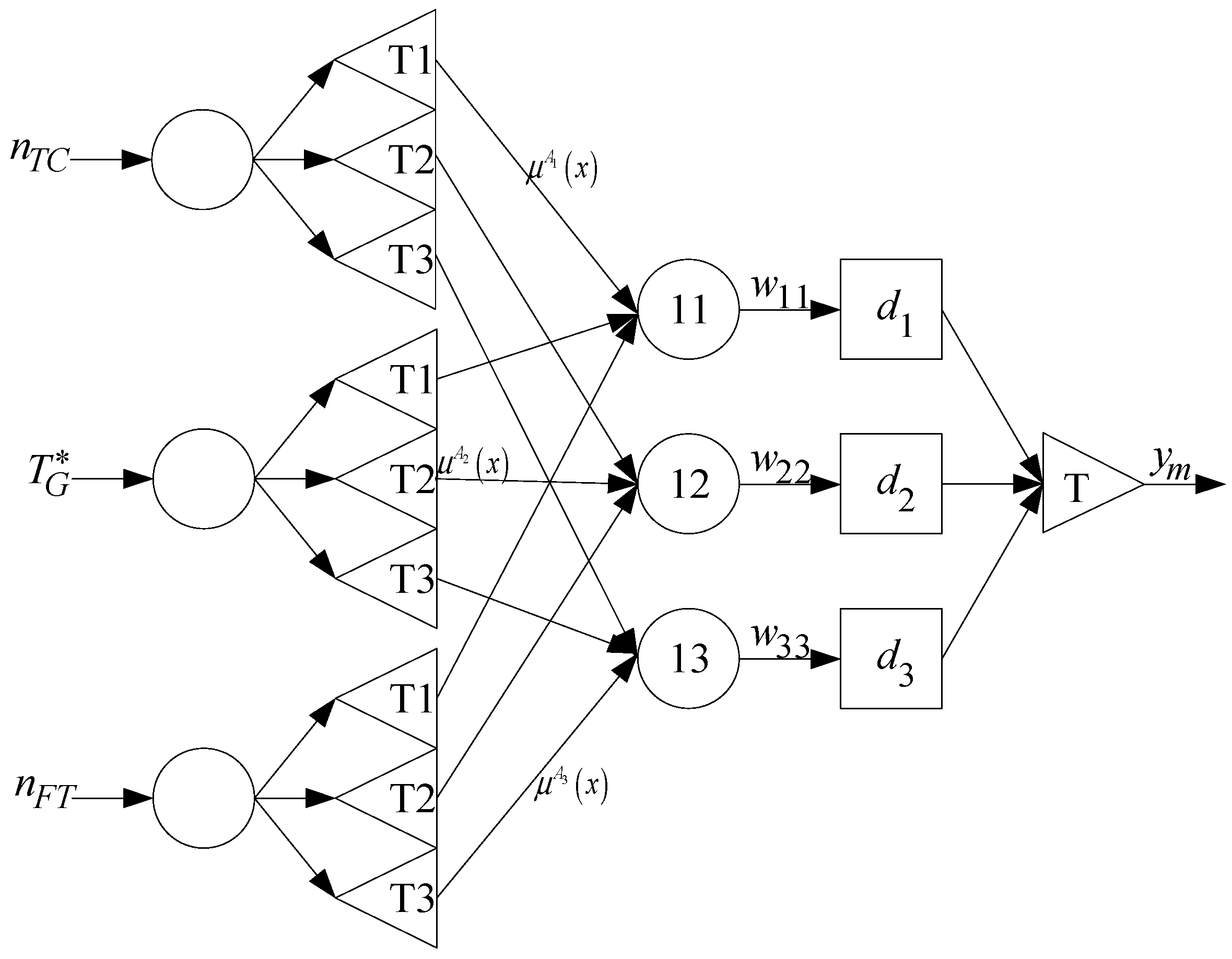
To solve the HTE controlling task, in [28] a hybrid NFN of the ANFIS type (Figure 1) use was proposed, which contains 5 layers: the first layer is the nonlinear object inputs under research (HTE); the second layer is the layer of fuzzy terms, which are used in the HTE fuzzy knowledge base; the third layer is the fuzzy knowledge base (fuzzy rules) conjunction lines; the fourth layer is the output variable dj classes, which is associated with a reference sample known in the fuzzy knowledge base; and the fifth layer is the defuzzification layer, that is, converting the fuzzy output into a crisp number.

Figure 1.
Reconfigured modified closed TE ACS model.
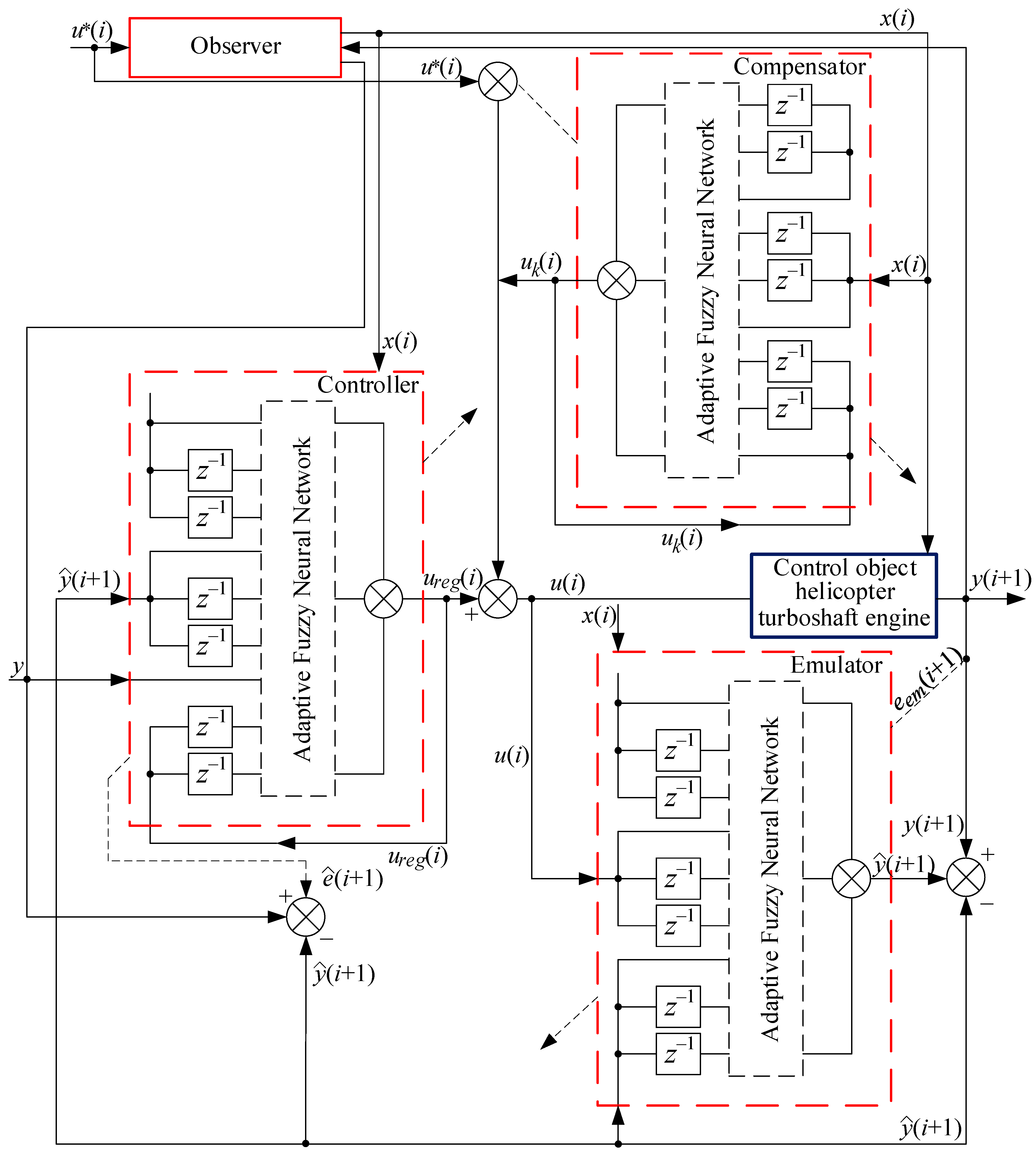
An key disadvantage of the ANFIS is its limited ability to adapt to complex and rapidly changing environmental conditions, which can lead to insufficient control accuracy in some scenarios. To eliminate these shortcomings, it is advisable to use an NFA ACS (Figure 2), proposed in [29], in which the influence of disturbing influences is largely eliminated by a compensator, and the control error e(i + 1) is eliminated by a controller, which is an adjusted emulator of an object model under research (HTE). This allows for more precise control in changing environmental conditions and improves the control system efficiency, especially in the context of dynamic objects such as HTE.
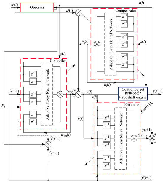
Figure 2.
Structure of an NFA modified closed TE ACS.
In Figure 2, the controller manages input signals for the system based on predefined rules and membership functions, ensuring the desired system behavior in changing conditions. The emulator simulates the dynamics of the controlled object, allowing the system to predict real object behavior and adjust controller actions for optimal performance. The compensator adjusts deviations from the desired system state, using feedback to minimize errors and stabilize system operation. The observer block evaluates the system state in real time, using sensor data and mathematical models to provide accurate information to the controller and other system components.
A neuro-fuzzy control system integrates principles from neural networks and fuzzy logic for effective management of complex dynamic objects. The controller makes decisions based on fuzzy rules that adapt to changes in the external environment. The emulator models object behavior, predicting responses to various influences, allowing the controller to make more accurate decisions. The compensator corrects deviations from the desired state, adjusting system actions to reduce errors. The observer block monitors object state in real time, providing up-to-date data for all system elements, enhancing their interaction and increasing control accuracy. Together, these components provide reliable and adaptive management capable of handling uncertainty and nonlinearity in controlled processes.
To account for the real-time aspect in a neuro-fuzzy control system, it is essential to implement efficient algorithms that process inputs and generate control signals within strict time constraints, ensuring timely responses to dynamic changes in the environment. This can be achieved by optimizing computational resources and employing parallel processing techniques to handle the system’s complex calculations without compromising speed or accuracy [32,33].
The controller, compensator, and emulator contain delay elements z(τ) = x(t − τ), τ = 1, 2,…, which form the input and output variables with a delay. Similar to (1), the compensator is described by a nonlinear difference equation form:
having orders qk and sk, differing in the general case from q and s, while uk(i − 1)…uk(i − qk) are scalar control actions, x(i) is a dimension v input disturbances vector, and ck is a parameters settings vector. The orders qk and sk indicate feedback delay and input signal delay, respectively. The introduction of a noise term (error) ϵk(i) into the compensator Equation (4) is justified by the need to take into account non-idealities and variable environmental conditions. In real-world conditions, measurements may be subject to noise, interference, or other external factors that may cause the compensator to operate inaccurately. In addition, even when using an accurate mathematical model, modeling errors and internal inaccuracies in compensator components, such as imperfections in design or calibration, are inevitable. The noise term introduction allows us to take these factors into account and make the compensator model more realistic, ensuring its better adaptability to real operating conditions.
According to [29], a replacement is introduced in (4):
where m = qk + v · (sk + 1).
Then (4) takes the form:
Based on [29], the Sugeno fuzzy model, represented by rules set, is used as the difference Equation (6) to describe the compensator:
with fuzzy sets , , , and a linear dependence connecting inputs , output uk(i), and noise term (error) ϵk(i).
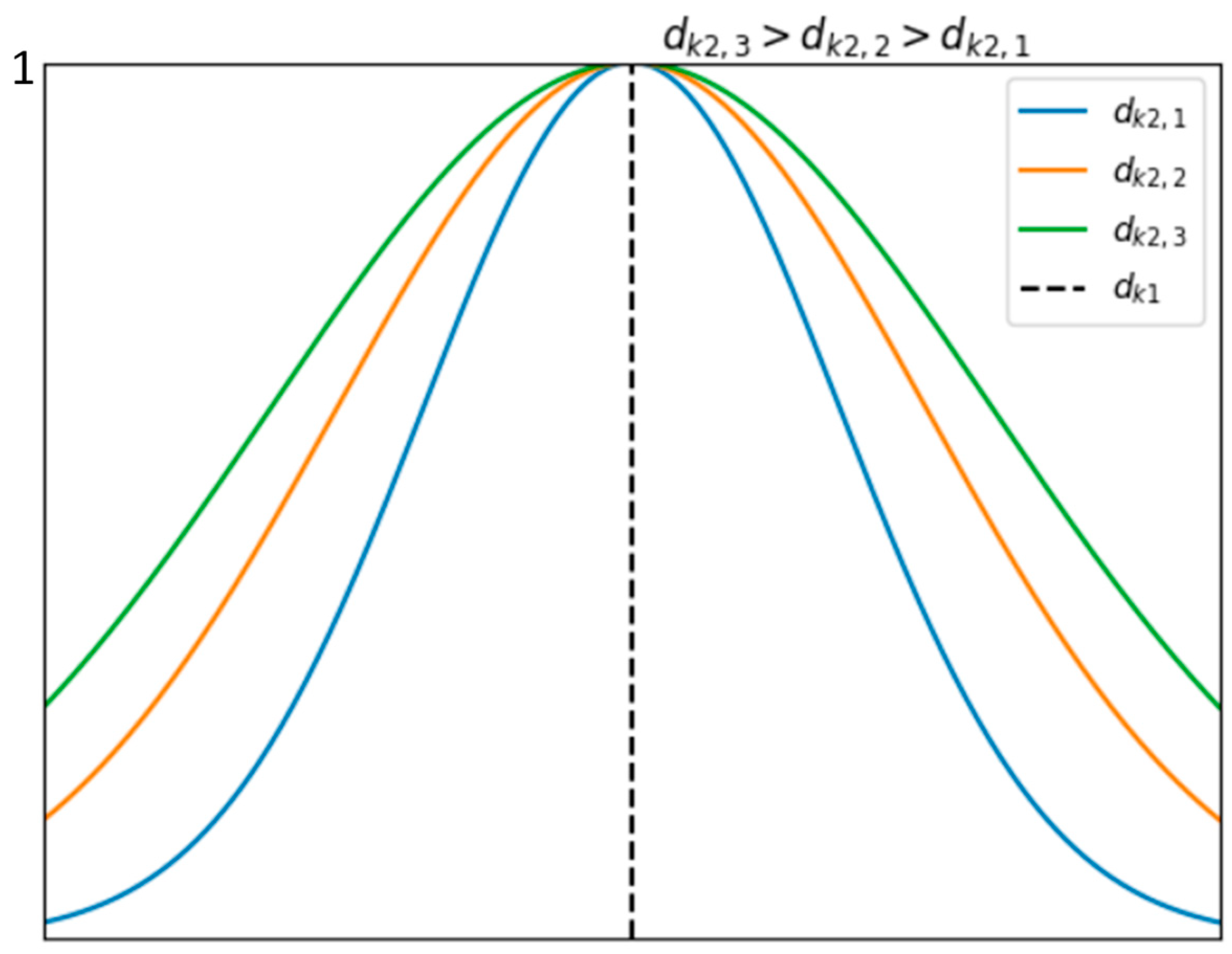
The main characteristic that defines the fuzzy set Xk is its membership function , which, according to [28], is a bell-shaped membership function (Figure 3) of the form:
where dk1 and dk2 are the bell-shaped membership function parameters.
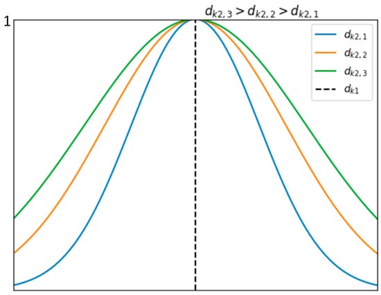
Figure 3.
Bell-shaped membership function general view.
According to [28], the fuzzy variable bell-shaped membership function use is justified in cases where it is necessary to more flexibly control the membership shape and distribution around the central value. Unlike the sigmoid function proposed in [29], which has a more limited range and faster saturation, the bell function allows us to more precisely tune the curve shape and adapt it to the system-specific requirements. This is especially useful in cases where there is a need to account for data uncertainty and varying degrees of fuzziness, or when there are multiple peaks in the distribution.
The choice of the bell-shaped membership function, as opposed to other types such as sigmoid functions, is primarily due to its superior flexibility in modeling fuzzy variables. The bell-shaped function, characterized by its smooth, symmetric curve, offers enhanced control over the shape and distribution around the central value, making it particularly effective in scenarios where precise tuning is required [34]. This function’s broader range and gradual saturation provide better adaptation to varying degrees of data uncertainty and fuzziness compared to sigmoid functions, which have a more constrained range and quicker saturation [35]. Furthermore, the bell-shaped membership function’s ability to accommodate multiple peaks in the distribution is crucial when dealing with complex systems exhibiting diverse operational conditions and varying degrees of uncertainty [36]. This flexibility ensures a more accurate representation of the system’s behavior and improves the overall performance of the neuro-fuzzy control model, aligning it more closely with specific system requirements and contributing to more reliable and adaptable control strategies.
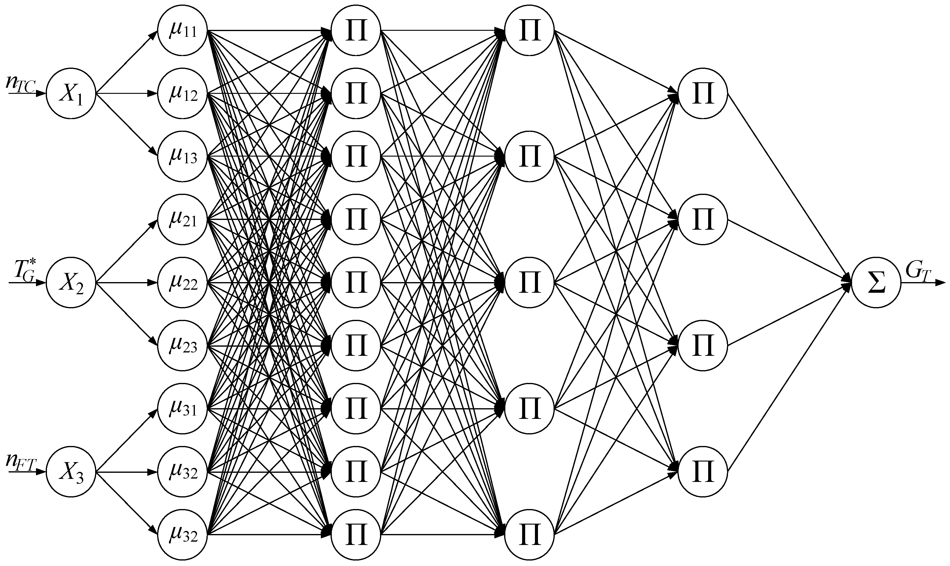
When determining the output uk(i) mechanism according to the fuzzy model (8) when specifying inputs at time i = 1, 2,…, N, membership functions , coefficients , and equation , taking into account [28,29], it is advisable to present it in an AFNN-type (adaptive fuzzy neural network) six-layer NFN form (Figure 4) [37].
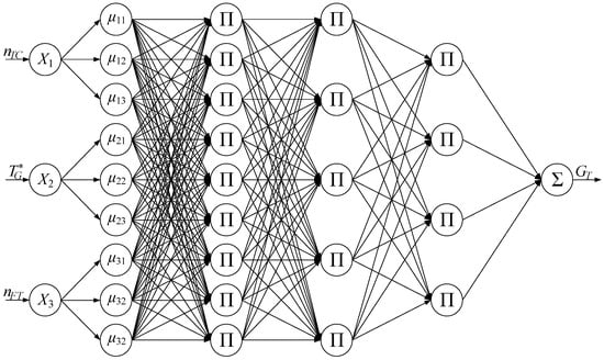
Figure 4.
Structure of the proposed AFNN-type six-layer hybrid NFN.
AFNN, based on the Sugeno model, is more appropriate for the neuro-fuzzy HTE ACS constructing task than ANFIS [28] or TSK models [38], due to its ability to handle uncertainty and nonlinearity in the system using a combination of FL and NNs. The Sugeno model provides a more flexible mechanism for describing fuzzy rules, which allows the system to better adapt to different HTE operating conditions. In addition, an AFNN using the Sugeno model can better adapt to changing conditions and requirements, thanks to a more complex network structure and the ability to train not only membership function parameters, but also neuron weights, which reduces the need to manually tune the system for each specific situation.
The Sugeno-based AFNN model offers significant advantages over traditional models like ANFIS or TSK for HTE neuro-fuzzy control systems. Its ability to handle uncertainty and nonlinearity through a combination of FL and NNs provides a more flexible mechanism for describing fuzzy rules, enabling better adaptation to varying operational conditions. Additionally, the Sugeno-based AFNN can more effectively adjust to changing conditions and requirements due to its complex network structure and the capability to train both membership function parameters and neuron weights, reducing the need for manual system adjustments [39,40].
As mentioned above, AFNN based on the Sugeno model consists of six layers. The first layer (Input Layer) accepts model input data, which are the HTE TDP numerical values, recorded on board the helicopter at flight mode: gas-generator rotor r.p.m. nTC, free turbine rotor speed nFT, and gas temperature in front of the compressor turbine .
In the second layer (Fuzzy Layer), the input data are converted into fuzzy values using membership functions (8) by calculating the membership degrees for θ-th rules.
In the third layer (First neural layer), the truth values of premises are calculated by algebraic multiplication:
The premises truth values calculation is a critical stage that determines the contribution of each premises to the corresponding rule activation. These values are each input variable membership degree’s product for a given rule θ, which reflects the model confidence degree in fulfilling the input data rule given conditions. Thus, high values of indicate a stronger coincidence of the input variables with the rules, which makes it possible to effectively take into account fuzziness and uncertainty in the data and generate correct output recommendations or HTE ACS control signals.
In the fourth–second neural layer, relative normalized values are determined as:
where α is a coefficient that can be adjusted during the network training process or determined based on additional expert information. The α coefficient allows more flexibility in each parcel contribution controlling to the normalized values, which can be useful if some parcels have greater meaning or significance than others.
In the fifth layer (Combining Layer), the outputs from the neural layer are combined using fuzzy methods or aggregation to produce the final model output. The values are multiplied by the output values , calculated according to the equation when setting the values , …, .
where is the k-th rule membership degree for the i-th input data, is the θ-th rule bias parameter, is the weighting coefficient for the j-th input in the θ-th rule, is the j-th input neuron for the k-th rule, and ϵk(i) is the additional error (noise).
Expression (11) is the product of the weights and outputs for each θ-th rule and each k-th input, which allows us to aggregate the contribution of each rule and its weighted output to the NFN final output.
The noise term (error) ϵk(i) is a random variable that represents the difference between the actual output value and its predicted or expected value at the i-th time moment. Mathematically, it is described as a random variable with zero mean and some variance, which characterizes the spread between the actual and predicted values.
In the sixth layer (Output Layer), after multiplying and combining the outputs for all rules, the final NFN output signal is calculated, which is an aggregated representation of output values, reflecting the calculated predictive or control recommendations based on the input data and parameters of the trained network:
2.2. Compensator Model
Based on [29], in the compensator fuzzy formulation, the vector tuning parameters ck are formed from the coefficients involved in the equations , as well as from the parameters , , related to the bell-shaped membership function shape. At the initial stage of setting up the compensator, the available data are used to determine the fuzzy rules number n using the structural identification algorithm ψn, the equations coefficients using the parametric identification algorithm ψb, as well as the parameters , using the backpropagation algorithm. In this case, data , u*(i) are used, for which the next output variable y(i + 1) value is close to the nominal ynom, such that it satisfies the condition [29,41]:
where Jnom is the relative control error nominal value.
Thus, for the compensator model mathematical description, it is advisable to research the structural identification algorithms [37], parametric identification [38], and the backpropagation algorithm [39].
The algorithm for identifying the equation coefficients , performed on the data set , u*(i), based on (7), (9), (10), (12) is represented in the forms:
or in vector form
where is the extended input vector, and is the vector of adjustable coefficients. To determine the initial values of the elements of the vector and the correction matrix of size [29,38,42]:
where φk is a coefficient that is a fairly large number, which is selected experimentally.
For the data set , u*(i), the correction matrix is calculated:
and coefficient vector
where λ is the regularization parameter. The desired value of the vector is equal to .
In the proposed modification, in contrast to [29], a regularization term is added to the coefficient correction process. This helps reduce overfitting and improve estimation robustness. The parameter λ must be carefully selected, since large values of λ can lead to underfitting, and too small ones can lead to insufficient consideration of regularization. The proposed method with regularization is especially useful when working with data prone to noise or with high multicollinearity between features.
The conducted research made it possible to formulate a theorem on the convergence of a modified parametric identification algorithm with regularization.
Theorem 1.
If the correction matrix Hk(i) satisfies the condition of positive definiteness at each i-th step, and there is also a constant μ > 0 such that λ ≤ μ, then the sequence converges to the true values of the coefficients bk, which minimize the model estimate root mean square error.
Proof of Theorem 1.
It is assumed that the difference between the current and next iteration steps is described by expression (18). Using the properties of the adjustment matrix Hk(i) and the regularization conditions , the sequence converges to the true values of the coefficients bk, since each iteration step reduces the model estimation error, taking regulation into account. Analyzing the iteration process dynamics and the adjustment matrix Hk(i) properties, we can establish that the sequence converges to the true values of the coefficients bk, minimizing the model error. □
Thus, the theorem on the modified parametric identification algorithm convergence with regularization confirms that when the adjustment and regularization matrix positive definiteness conditions are met, the sequence of coefficients converges to the true model parameters, which completes the proof of the theorem.
To start the structural identification algorithm ψn operation, according to [29], a fuzzy model with the lowest criterion value is selected:
From the available models, the one with the lowest criterion value is selected. If only one model is available, for example in the first iteration, this step is skipped. The resulting fuzzy model is then trained on the current data by systematically correcting the coefficients using a multi-step least squares method (Equations (17) and (18)) and the membership function parameters , using the backpropagation algorithm [34], which aims to minimize the squared error:
using the gradient method according to the expression
with working step , where hk is the working step parameter.
The chain rule for determining the partial derivative according to [29] has the form:
where is the bell-shaped membership function (Figure 3) parameters’ two-element vector. Each component of the partial derivative (22) is determined according to (8)–(12). In this case, according to (20), it is defined as:
the components of which are determined: according to (20), according to (7) and (10), according to (9), and as the bell-shaped membership function derivative with respect to or :
Since according to (9) , (25) is rewritten as:
Taking into account (24)–(27), (23) is presented as:
or
The resulting expressions (29) and (30) are modified in comparison with similar ones [29] by taking into account the noise term (error) ϵk(i) and the network training tuning coefficient α, as well as the bell-shaped membership function rather than the use of a sigmoid one.
The physical meaning of the derivative is to measure the sensitivity of the error ϵk to changes in the variable in the context of the compensator model. This derivative shows how changing the value, which can be a parameter or input value of the model, affects the error ϵk. If the value is large, this indicates that small changes in can lead to large changes in the model error ϵk, which may be important to optimize model parameters or analyze its sensitivity to certain input data. This can also help in understanding which factors or variables have the greatest impact on the NFA modified closed HTE ACS compensator model (Figure 2) accuracy and stability.
This modification makes it possible to improve the model accuracy and generalization ability, taking into account the data characteristics and the noise level in them, provide more flexible approximation, and allow the model to better adapt to different data types, which in turn contributes to more efficient training and prediction results.
2.3. Emulator Model
The emulator is an HTE simplified dynamic model, which can be described by a mathematical equation. This emulator is a real engine abstraction, taking into account the basic physical and technical characteristics, but not including all the details and complexities inherent in the real device. It is used to analyze the HTE operation and simulate in various modes and conditions, allowing researchers and engineers to test and optimize control systems and engine parameters without involving the large resources and time costs associated with real tests. Helicopter TE emulators can also be used for training and ensuring safety in the helicopter operational operation, allowing engine behavior analysis in various situations and flight conditions. Based on (1), the emulator is described by the equation:
where represents the output signal next value prediction at time i + 1 according to the emulator model, and g(•) is the emulator function that takes into account the current state , disturbance vector x(i), control u(i), an additional parameter g(i), and a tuning parameters vector.
A tuning parameters vector in the context of an emulator means averaging by this vector all components over time or over the entire available data sample. For example, if it represents an emulator model settings vector (such as weights or coefficients), then is a vector whose every component is the corresponding vector component average. Thus, if , then
Based on [29], expression (31) has known orders r, s, q, similar to (1). After formalizing the variable , expression (31) is also represented in the form of a fuzzy Sugeno model:
The analytical expression of a fuzzy emulator, presented in a six-layer AFNN form, similar to (12), has the form:
in which, similarly to (9) and (10), and are calculated as:
The coefficient αem in an emulator model is a tuning parameter or weight that is used to control the contribution of each parameter or characteristic to the model’s calculations. The αem parameter allows us to more flexibly take into account the significance of each element of input data or the influence of model parameters on its output. Thus, the coefficient αem scales or adjusts the significance of in the controller model. Similar to the α coefficient in NNs, the αem parameter is tuned or determined based on expert knowledge or the emulator model training process to achieve optimal model performance or accuracy in modeling and control tasks.
The algorithm for identifying coefficients bem(i) is identical to (14)–(18), that is:
where λem is the regularization parameter, is the modified input vector, and is the adjustable coefficients vector.
For structural identification, as in [29], a similar criterion (19) is used, characterizing the average relative error:
The emulator bell-shaped membership function parameters , are determined by the backpropagation method by minimizing the quadratic discrepancy similarly to (20) as:
using the gradient method according to the expression
with working step , where hem is the working step parameter.
The chain rule for determining the partial derivative according to [29], similar to (22), has the form:
which, after mathematical transformations similar to (24)–(28), is represented as:
or
Parametric and structural identifications stop when a condition similar to (13) is met:
where Jem is the emulator average relative error with an acceptable nominal value of the relative error Jem nom.
2.4. Controller Model
In an NFA modified closed onboard HTE ACS (Figure 2) with a regulator, emulator, and compensator, the regulator is a system part that takes as input the system current state and issues a control action to correct this state in accordance with the desired requirements or control aims. The controller uses fuzzy rules and a knowledge base to make control decisions based on current historical data and input variables.
To construct a controller model according to [29], it is assumed that the HTE described by (1) is reversible, that is, there is a controller model function fp(•) of the form:
in which the values i − r + 1, i − s + 1, i − q + 1 indicate specific points in time in the past (relative to the i-th point in time), which are taken into account when determining the variables that the controller model ureg(i) influence. These values are used to evaluate the system state and input variables in the past in order to make a decision on the necessary control action ureg(i) at the current i-th time. The variable ynom represents the system state nominal value y, which is likely used in the controller model to compare with the system current state and calculate the corrective control action.
After formalizing the variable expression (46) is also represented as a fuzzy Sugeno model of the form:
The fuzzy controller analytical expression is similar to (12), taking into account [29], and has the form:
which is a control actions weighted average from all controller components multiplied by its weight and then divided by the all-weights sum . This makes it possible to take into account the contribution of each component in the overall control action formation. The coefficient αreg is multiplied by this weighted average result, which serves as an adjustment or the controller output control action ureg(i) scaling. In (48), similarly to (9) and (10), and are calculated as:
where is a modified input vector.
According to [29], inverse controller model structure and parameters identification is carried out in two stages. At the first stage, we use the emulator model and a one-dimensional search algorithm at the points and, accordingly, the regulatory influences , at which the emulator error satisfies the constraints , .
At the second stage, structural identification and linear equations coefficients identification and the bell-shaped membership functions parameters are carried out. The coefficients vector is calculated using the recurrent least squares method identical to (14)–(18), that is:
where λreg is the regularization parameter, is the vector adjustable coefficients, and Hreg(0) = γ · I, .
For structural identification, as in [29], a similar criterion (19) is used, characterizing the average relative error:
Structural and parametric identification is completed when a condition similar to (13) is met:
where Jreg is the emulator average relative error with the permissible nominal value of the relative error Jreg nom.
The emulator bell-shaped membership function parameters , are determined by the backpropagation method by minimizing the quadratic discrepancy similarly to (20) as:
using the gradient method according to the expression
with working step , where hreg is the working step parameter.
The chain rule for determining the partial derivative according to [29], similar to (22), has the form:
which, after mathematical transformations similar to (24)–(28), is represented as:
or
2.5. Clarifying the Emulator Model Taking into Account the Controller Model
Taking uk constant, and taking into account that ureg = xem1, i.e., dureg = d(uk + ureg) = dxem1 according to [29], the object analytical Jacobian expression is defined , which is the sum of derivatives of the products of two functions βθ and :
Based on [29] in accordance with the chain rule, the first term total derivative has the form:
where
Taking into account (62), expression (61) takes the form:
The advantage of (63) over [29], where a similar expression is represented as , consists in its ability to take into account multidimensional interactions and nonlinear effects between variables through complex weighting coefficients and derivatives, which makes it possible to more accurately model dependencies in a multidimensional NFA modified closed HTE ACS (Figure 2).
2.6. Six-Layer NFN AFNN Training Algorithm
At the training initial stage, a parameter based on a six-layer NFN AFNN, xk(i) is accepted as the k-th input parameter for the i-th sample in the training set. The fuzzy transformation in the fuzzy layer uses the membership functions to transform xk(i) into the fuzzy value , that is, .
For each θ-th rule and each premise k, the premises truth degrees are calculated as:
Next, for each rule of the θ-th rule and each premise k, the relative normalized value is calculated, taking into account the parameter α, as:
The next training step is to define a loss function L that measures the difference between the actual output y(i) and the model predicted output ŷ(i):
where ϑ is the coefficient that regulates the influence of the adaptive multiplier, and t is the current training epoch number, the introduction of which into (66) allows us to adapt the loss function during the training process contribution. By adding the term to (66), in which λ is the regularization coefficient and is the L2-norm of the model parameters θ, it is possible to model the complexity control by penalizing large parameter values. The regularization coefficient λ determines the regularization strength: large values of λ increase the penalty for large parameters, which can help prevent overfitting.
For each θ-th model parameter, its gradient is calculated using the chain rule and gradient descent as:
Using gradients, the model parameters θ are updated using the gradient descent method:
where ηt is the current adaptive training rate at the t-th step. The training rate becomes adaptive by applying algorithms such as Adam or RMSprop [42,43], which automatically adapt the learning rate based on the gradient history.
Thus, adding adaptive elements to the training algorithm for a six-layer NFN AFNN will allow the HTE ACS to change its parameters and settings in real time based on changing conditions or external influences. The proposed algorithm can use feedback data to automatically adjust system parameters to achieve optimal performance even under variable conditions.
2.7. Observer Block Introduction into an NFA Modified Closed Onboard TE ACS
For a modified nonlinear difference system (1), where only the output measurements y(i) are available, and the state x(i) is not available for direct measurement, to estimate the system state x(i) based on the available measurements of y(i) and control actions u(i), the use of an observer block is proposed. It is assumed that the system state x(i) evolves in accordance with the discrete dynamic equation:
where v(i) is a noise or disturbances vector, and the function g describes the changes dynamics in the system state based on the current state x(i), control u(i), and disturbance v(i).
The observer block aim is to estimate a state that is approximately equal to the real state x(i) using available measurements y(i) and control inputs u(i).
One observer method for discrete systems that can have significant advantages over the Extended Kalman Filter (EKF) is the Matching State Observer algorithm—the Innovation Matching Observer algorithm [44]. The state-matching observer algorithm advantage over the extended Kalman filter is its simplicity and the absence of the need to linearize nonlinear measurement functions, making it more efficient and robust for nonlinear systems.
The basic idea of the Matching State Observer method is to use measurements of y(i) to directly determine x(i), minimizing estimation error. This method’s advantage is its simplicity and efficiency, especially in cases where the measurements are directly dependent on the state of the system.
According to the Matching State Observer method, the system state prediction is defined as:
where is the system state current assessment, and A and B are the system or control matrices.
Measurement-based state correction (update) is defined as:
where C is the measurement matrix that the system state relates to measurements y(i), and K(i + 1) is the observer gain matrix, which is chosen to the estimation error minimize, which is defined as:
where P(i + 1) is the state covariance error estimate, and R is the measurement noise covariance matrix.
This observer method directly uses measurements of y(i) to adjust the state estimate , which can be an effective way to estimate state in discrete systems, especially if the measurements have a direct and reliable relation with the system state. It also has a simple implementation and does not require the nonlinear measurement function linearization, which can be an advantage over the extended Kalman filter in certain scenarios.
3. Results
3.1. Input Data Analysis and Pre-Processing
To test the developed NFA modified closed onboard HTE ACS, including a controller, compensator, emulator, and observer unit, implemented in the six-layer NFN AFNN form, a computational experiment was carried out, for which a personal computer with a processor was used, i.e., AMD Ryzen 5 5600, 32 KB L3 cache, Zen 3 architecture, six cores, 12 threads, 3.5 GHz, RAM—32 GB DDR-4.
The data used to train the neural network include the HTE thermodynamic characteristics collected during flights, such as gas-generator rotor r.p.m. nTC, free turbine rotor speed nFT, and gas temperature in front of the compressor turbine . The developed NFA modified closed onboard HTE ACS initial data were obtained from experimental research conducted on the TV3-117 engine (Table 1) [26,27,45,46,47].

Table 1.
Initial data fragment for the developed NFA modified closed onboard TE ACS.
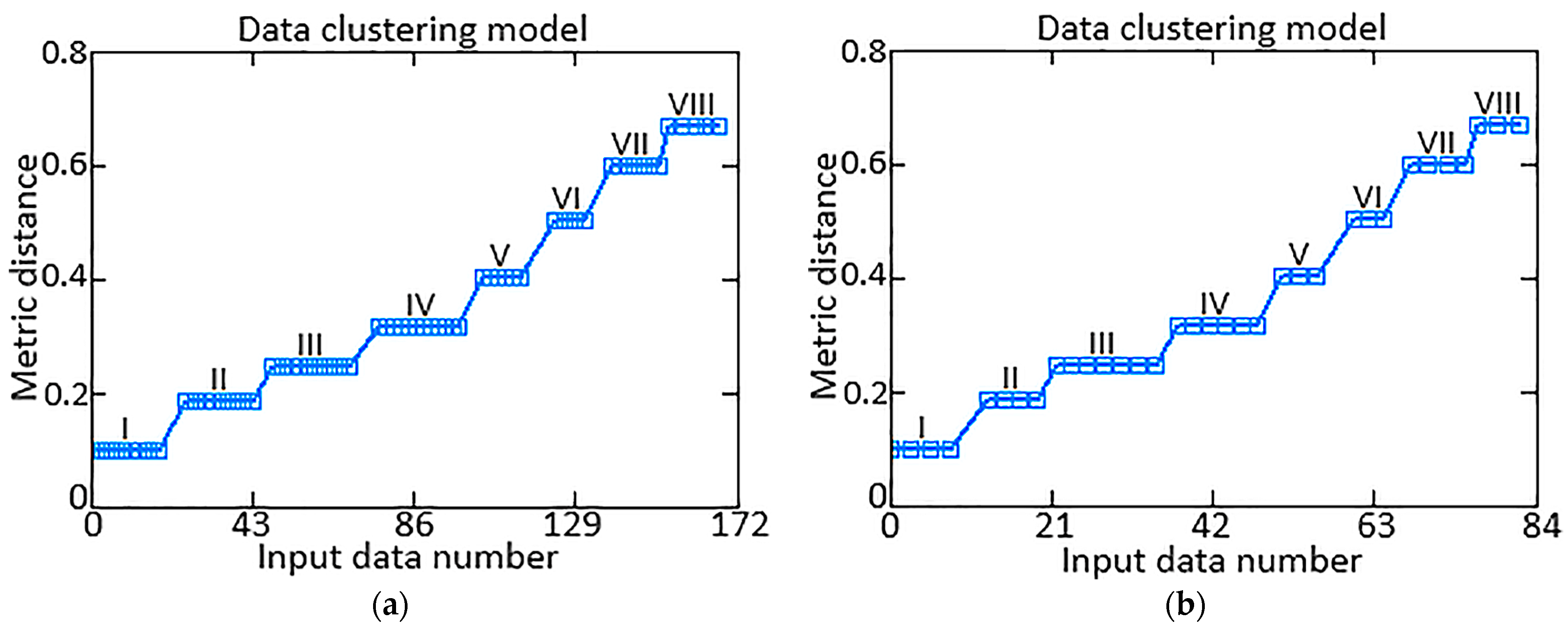
The input data (the training set) pre-processing is given in [26,27,45,46,47]. As part of the input data preliminary processing, it was proven that the training set is homogeneous according to the Fisher–Pearson [48] and Fisher–Snedecor [49] criteria, whose values were 3.588 and 1.28, respectively. The obtained values of these statistical criteria are less than their critical values (22.362 and 3.44, respectively), with 13 free powers and a 0.01 significance level. According to [26,27,45,46,47], a control sample (67%) and a test sample (33%) were separated from the training sample (Table 2), and this representativeness was confirmed by cluster analysis [50,51] using the k-means method, during which the input data values were divided into eight classes and the metric distance between them was calculated as , in which μj are the initial centroids and is the Euclidean distance between xi and μj (Figure 5). In this case, the μj values are recalculated as , which is the number of objects in the j-th cluster. Calculations of Ci and μj continued until changes in the cluster distribution became negligible.

Table 2.
Results of forming training, control, and test samples (author’s research).
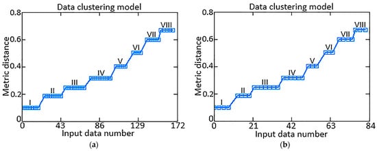
Figure 5.
Cluster analysis results: (a) original experimental dataset (I…VIII–classes); (b) training dataset.
Similar research was conducted, during which the following were separated from the training sample (Table 2) and identified: a control sample (60%) and a test sample (40%); a control sample (50%) and a test sample (50%); a control sample (70%) and a test sample (30%). The obtained metric distance values with such combinations are 1.75…3.38 times greater than with the control sample (67%) and a test sample (33%). This indicates the optimal choice of control and test sample size.
Thus, the training sample elements’ preprocessing results made it possible to form the optimal training, control, and test sample sizes (Table 2).
3.2. The Six-Layer NFN AFNN Training Results
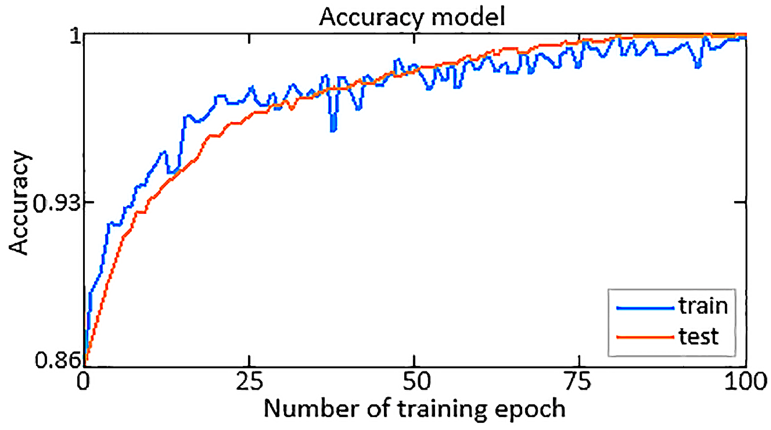
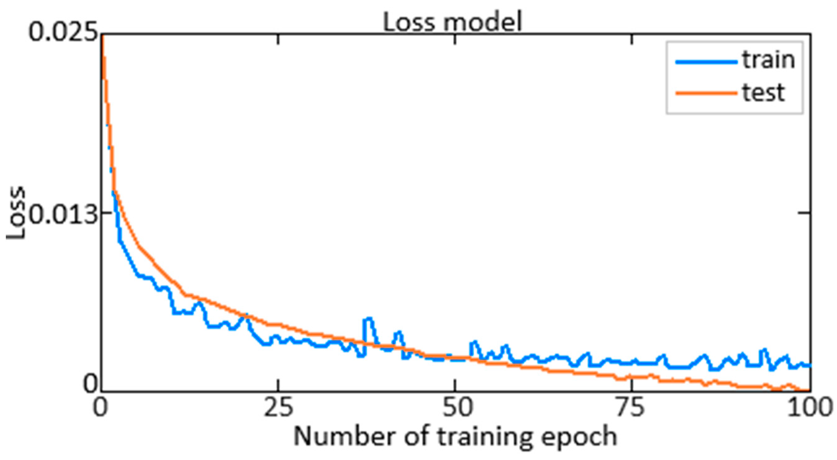
In the NFN AFNN training process with the proposed algorithm (64)–(68), the values of the accuracy (Accuracy) (Figure 6) and loss (Loss) (Figure 7) functions were estimated for the training and validation samples; the blue curve indicates training results on the training set, and the orange curve indicates validation results on the control set.
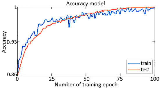
Figure 6.
Diagram of changes in the neural network accuracy function with 1000 iterations.
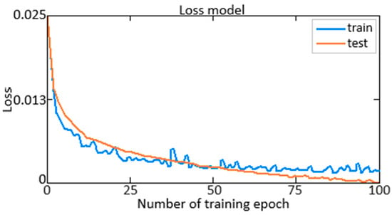
Figure 7.
Diagram of changes in the neural network loss with 1000 iterations.
The accuracy metric reflects the model effectiveness in determining the neuro-fuzzy HTE ACS parameters, showing the percentage of correctly calculated parameters. In turn, the loss function demonstrates the degree to which the model’s predictions deviate from the actual values, which helps optimize the training process by reducing this loss. By analyzing the resulting diagrams of the accuracy (Accuracy) (Figure 6) and loss (Loss) (Figure 7) functions during the training process, conclusions are drawn about how effectively the model is trained, and measures are taken to improve its performance.
According to Figure 6, almost maximum accuracy has been achieved, and according to Figure 7, the loss value does not exceed 0.025, which indicates the model’s high training efficiency on available data and its ability to accurately generalize to new data.
It is worth noting that for a bell-shaped membership function with 60 iterations, the value of the accuracy metric reaches 0.9998 (99.98%), and the value of the loss function does not exceed 0.0002 (0.2%), which indicates the high efficiency and accuracy of the AFNN network when using the bell-shaped function accessories. The results obtained indicate the successful training of the neuro-fuzzy AFNN network, with good convergence and minimal error, which emphasizes the importance of correct membership function choice in the design process of a neuro-fuzzy HTE ACS. At the same time, the loss values in both samples do not exceed 0.025 (or 2.5%), which indicates a low level of error in determining the neuro-fuzzy HTE ACS parameters. Such results indicate the successful training of the AFNN network with the proposed algorithm and its ability to provide the neuro-fuzzy HTE ACS accurate parameters with a high degree of confidence.
Determining confidence in the context of machine learning and neural network models typically involves assessing likelihood or the model’s confidence in its predictions. Depending on the type of model (e.g., classification or regression), the confidence degree can be expressed differently [52]. This work uses a method for assessing the AFNN network’s confidence which consists of using maximum probability. For classification problems, a softmax function is often used to determine the membership probabilities in each class. After model training, having received the prediction for input data x, we can obtain the probability belonging to the k-th class using softmax:
where is the model outputs vector before applying softmax for input x, is the vector k-th element, and K is the class number.
Figure 8 shows a diagram of the maximum probability (Max Probability Estimation) for the AFNN network “degree of confidence”, which shows how the AFNN network confidence in obtaining the neuro-fuzzy HTE ACS parameters is distributed: (a) is the nTC parameter, (b) is the nFT parameter, and (c) is the parameter.

Figure 8.
Maximum probability estimation diagram for “degree of confidence”: (a) is the nTC parameter, (b) is the nFT parameter, and (c) is the parameter.
Table 3 presents the comparative analysis results of the accuracy metric and the loss function calculations when using various membership functions in the AFNN network training process using the proposed algorithm (64)–(68).

Table 3.
The different membership functions comparison results.
In the process of training the NFN AFNN, similarly to [28,29], the bell-shaped membership function (Table 4) parameters were updated using an adaptive training rate according to the expressions:
where ηt is the current adaptive training rate at the t-th step.

Table 4.
The bell-shaped membership function parameters values before and after training of AFNN neural fuzzy network (author’s development, based on [28]).
The quality of the bell-shaped function parameters calculating and according to (74) using the adaptive training rate in comparison with the expressions , , applied in [28], was estimated by the values of RMSE (square root of root mean square error), MAE (mean absolute error), and MAPE (average absolute percentage error):
where n is the number of obtained values and , and are actual values of i-th parameters and , and and are the calculated NFN (AFNN in this work, ANFIS in [28])values of i-th parameters and .
Table 5 shows the calculated RMSE, MAE, and MAPE value results for the bell-shaped membership function parameters and . Table 4 shows that for the RMSE value is 0.0524, MAE is 0.0537, and MAPE is 5.0011% when applying (74). At the same time, the RMSE value is 0.0765, MAE is 0.0816, and MAPE is 7.6516% when applying the expressions from [28], , . Similarly, for RMSE is 0.0521, MAE is 0.0536, and MAPE is 5.0008%, and when using expressions from [28], RMSE is 0.0761, MAE is 0.0815, and MAPE is 7.6512%. Thus, the results obtained indicate a decrease in the RMSE, MAE, and MAPE values for the bell-shaped membership function parameters and by 1.46, 1.52, and 1.53, respectively, when applying (74), adaptive speed training, compared with [28].

Table 5.
Values of statistical criteria RMSE, MAE, and MAPE.
Thus, the work experimentally confirmed the feasibility of an adaptive training rate for introducing the NFN AFNN.
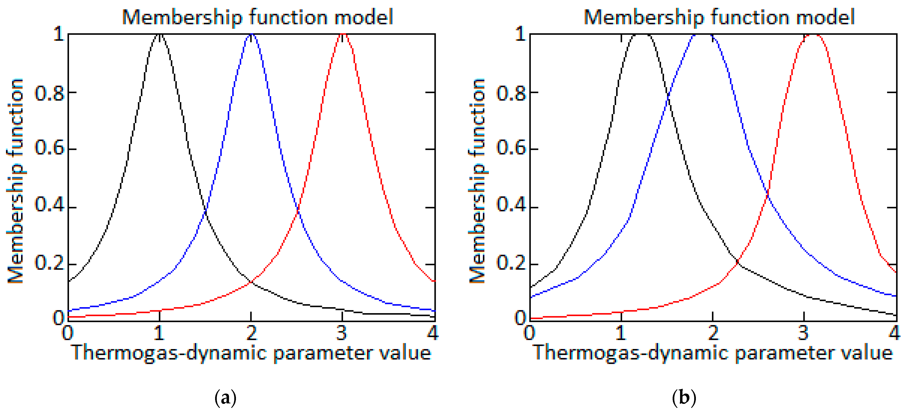
The obtained results of bell-shaped function parameters and made it possible to graphically represent the bell-shaped membership function appearance. Figure 9a shows the bell-shaped membership function appearance before training the AFNN NFN using the initial parameters and , and Figure 9b shows the same after training the NFN AFNN with refined parameters and . The refinement of parameters and of the bell-shaped membership function is justified by “fine-tuning” the fuzzy model of the research object, an NFA modified closed onboard HTE ACS. After parameter optimization, the bell-shaped membership function underwent changes, resulting in a more accurate fit to system data. These changes improved control quality by adapting the function to the controlled object (HTE) specifics.
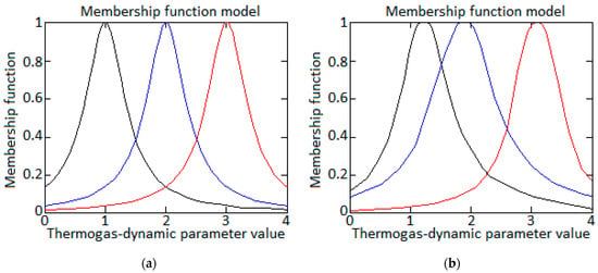
Figure 9.
Bell-shaped membership function: (a) before training the NFN AFNN, (b) after training the NFN AFNN [28,52].
3.3. Computational Experiment Results
During the next phase of the computational test, the neuro-fuzzy HTE ACS parameters, which are based on a six-layer neuro-fuzzy AFNN network, were directly determined. As a result of modeling changes in the HTE thermogas-dynamic characteristics according to the training sample data (Table 1) at various moments of model time (from 0 to 5 s), the conclusions are shown in Figure 10, where (a) means the change in nTC, (b) means the change in , and (c) means nFT. The orange curve represents experimental data on TDP recorded on board a helicopter, while the blue curve shows the model values of these parameters after correction using a reconfigured helicopter TE ACS [28], and the black curve shows the model values of these parameters after correction using the proposed neuro-fuzzy HTE ACS (Figure 2).

Figure 10.
Results of modeling changes in the TE thermogas-dynamic characteristics in the time interval from 0 to 5 s: (a) parameter nTC change, (b) parameter change, (c) parameter nFT change.
To confirm the obtained curves’ adequacy as a result of modeling, the study used the determination coefficient R2 as a statistical criterion for comparing the curves. This criterion evaluates the degree of agreement between model (blue curve and black curve) and experimental data (orange curve); a value close to 1 indicates a good fit of model data.
The percentage deviation from the experimental curve can be calculated as the ratio of the difference between the model curve values and the experimental curve to the experimental curve value, multiplied by 100%, according to the expression:
where xi is the i-th point on the model curves (blue curve and black curve), and is the i-th point on the experimental curve (orange curve).
To calculate the determination coefficient R2, 50 points were taken on the model and experimental curves with a uniform step of 0.1 s. The determination coefficient for the blue curve obtained using a reconfigured HTE ACS [28] was 0.916, and for the black curve obtained using the proposed neuro-fuzzy HTE ACS (Figure 2)—0.982. Thus, the value of the determination coefficient for the proposed neuro-fuzzy HTE ACS (Figure 2) is 1.07 times higher than the value of the determination coefficient for the reconfigured HTE ACS [28], which indicates better adequacy and accuracy of the proposed HTE ACS.
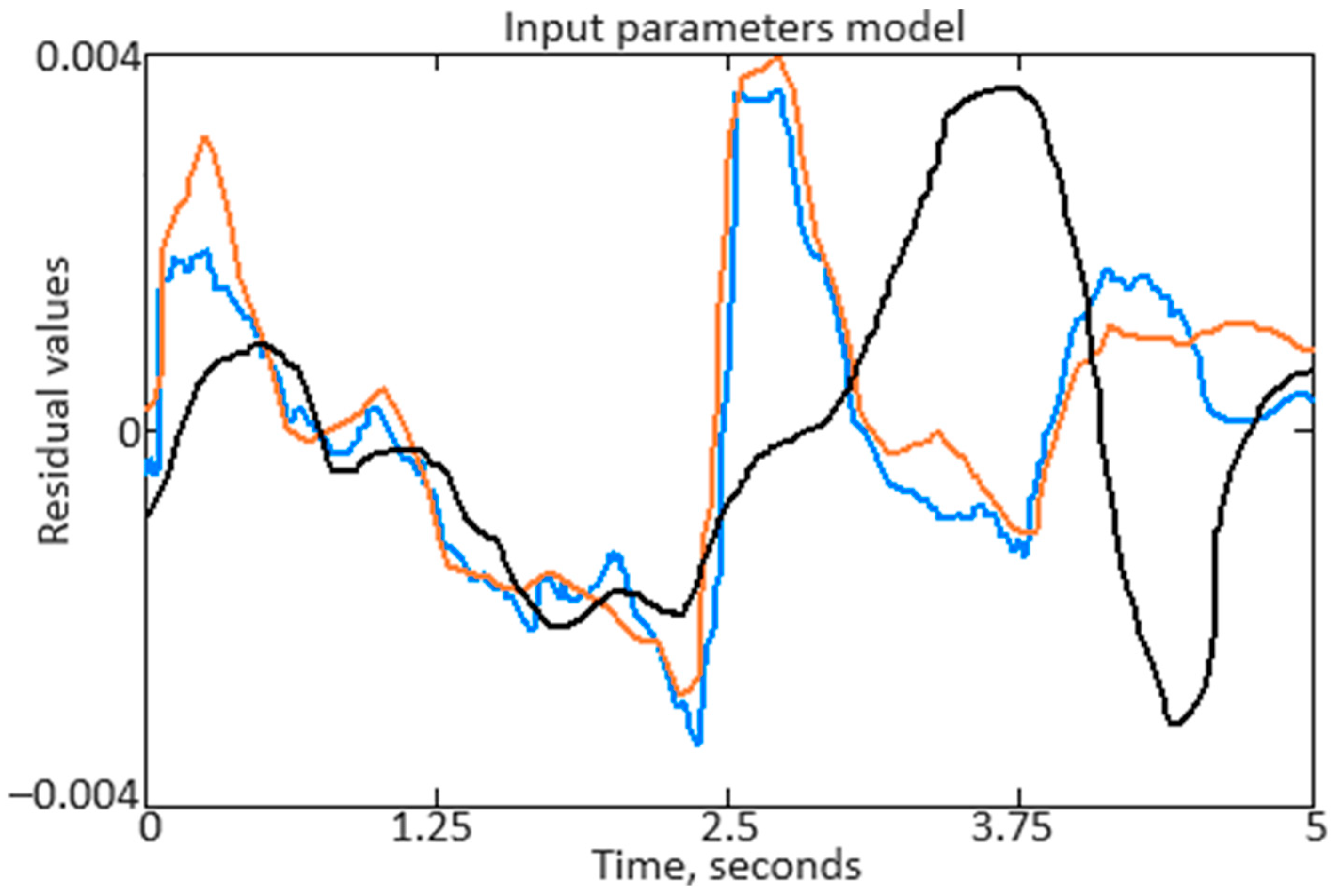
The change in residuals after regulation ε(t) = x1(t) + x2(t) + x3(t) − y(t) remains within the HTE TDP permissible deviation, not exceeding 0.004. These parameter dynamics, shown in Figure 11 after regulating ε(t), demonstrate the control stability, where the ε(t) value tends to zero.
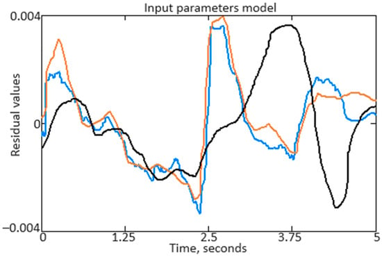
Figure 11.
Results of calculating residuals after regulation: orange curve—according to the nTC parameter, blue curve—according to the parameter, black curve—according to the nFT parameter [28].
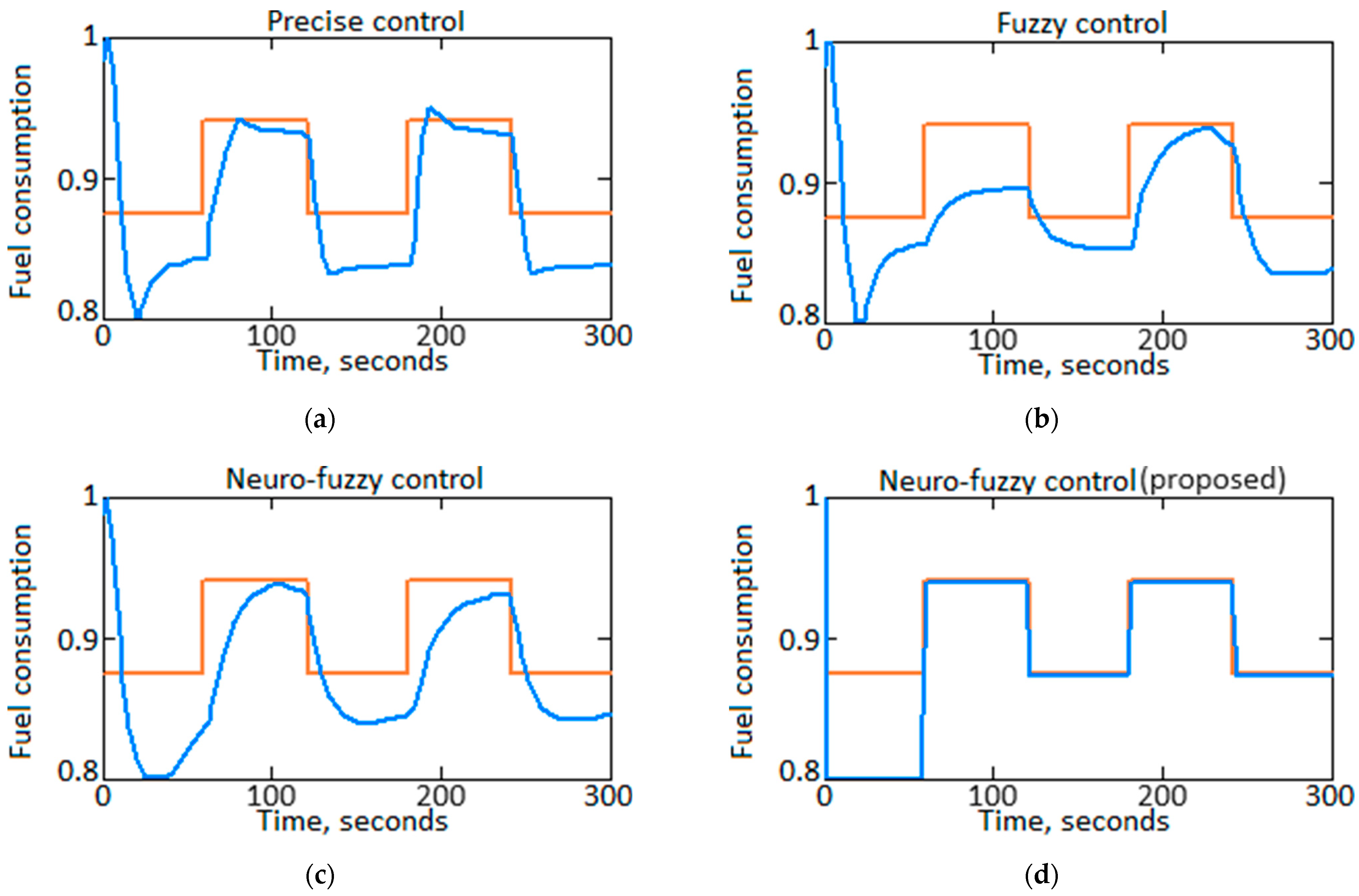
At the computational experiment’s next stage, the fuel consumption parameter GT was determined (in absolute units) for various control types (Figure 12, where the blue curve shows the reference value of fuel consumption GT (step action) and the orange curve shows the fuel consumption GT real value), while, similarly to [28], it was assumed that the fuel consumption parameter GT reference signal has a rectangular pulse form, that is, a step change in the required fuel consumption GT.
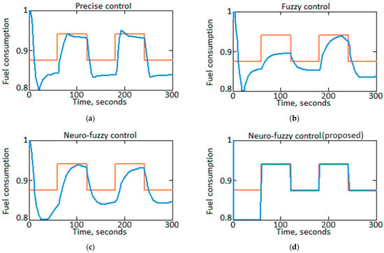
Figure 12.
The fuel consumption parameter GT (in absolute units) calculation results for the HTE TDPgiven values: (a) for precise control (traditional ACS), (b) for fuzzy control, (c) for neuro-fuzzy control using a reconfigured ACS) [28], (d) for neuro-fuzzy control using the proposed helicopter turboshaft engine neuro-fuzzy ACS.
From the presented transient control process analysis diagram (Figure 12), it is clear that the control quality (measured by the duration of the transient process and the maximum deviation of the controlled value) when using traditional (Figure 12a), fuzzy (Figure 12b), and neuro-fuzzy (Figure 12c) control types are approximately the same. At the same time, when using neuro-fuzzy control using the proposed neuro-fuzzy HTE ACS (Figure 12d), the transient process duration and the controlled value GT maximum deviation are reduced by an average of 15…20% compared with the above-presented control types. The role of a compensator in neuro-fuzzy control lies in its ability to effectively compensate for uncertainties and disturbances in the ACS. The compensator predicts and corrects the influence of external factors, which allows the system to respond faster and more accurately to changing conditions, which ultimately led to an improvement in the control quality, with a reduction in the duration of the transient process and a reduction in the controlled value GT by 15…20% maximum deviation.
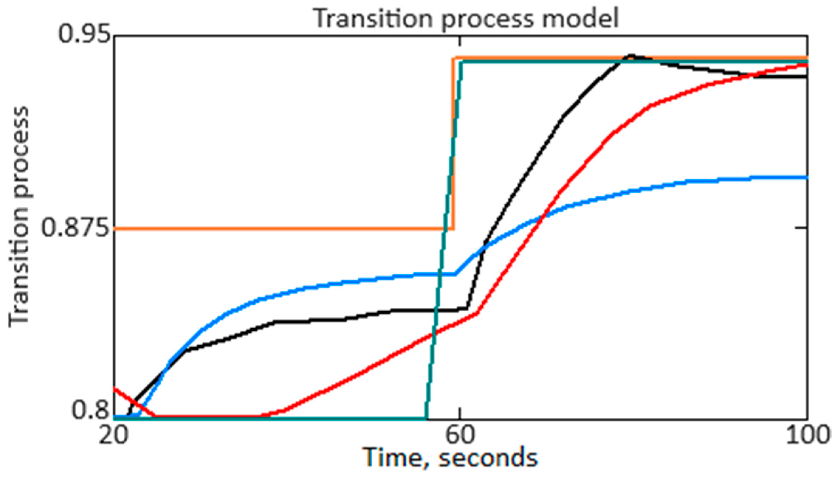
At the computational experiment’s next stage, detailed research on the fuel consumption GT parameter transition process section is carried out—from 20 to 100 s (Figure 12), where the orange curve is the fuel consumption GT real value, the black curve shows the transition process for precise control (traditional ACS), the blue curve shows the transition process for fuzzy control, the red curve shows the transition process for neuro-fuzzy control using a reconfigured ACS [28], and the green curve shows the transition process for neuro-fuzzy control using the proposed neuro-fuzzy HTE ACS.
To achieve the ACS stable operation, as well as to fulfill the transient processes’ specified quality indicators, according to [28,53,54,55], the synthesized system parameters’ quantities under consideration of dependence are studied:
where q1,…, qi are the quality indicators of the transient processes under consideration; {ki}, {τi}, {Ti} are the variable system parameter (gain factors, time constants, etc.) sets; f1(•), …, fi(•) are the functions expressing the system quality indicators’ dependence on the synthesized controllers parameters.
If we take overshoot and subsystem regulation time as the main indicators of system quality, then the system of Equation (79) takes the form:
where σ1,…, σi is the overshoot, and treg1,…, treg_i is the subsystems transient processes regulation time.
To determine the subsystems transient processes regulation time according to the transient process diagram (Figure 13), at the initial stage the establishment moment is determined, which indicates the time moment when the output quantity (controlled quantity) approximately stabilizes in the vicinity of the steady-state value. Next is the first point on the diagram (t1), at which the controlled value enters the vicinity of the steady value and remains in this vicinity further. Next is the last point on the diagram (t2), at which the controlled value leaves the steady value’s vicinity and no longer returns to this vicinity. The regulation time treg is defined as the difference between t2 and t1, that is:
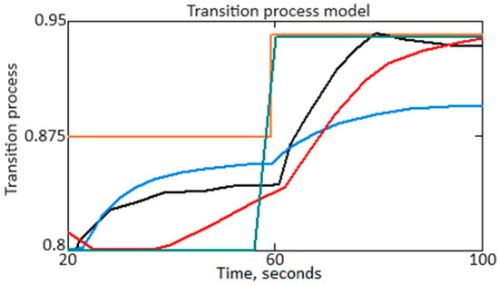
Figure 13.
Diagram of the fuel consumption parameter GT transition process (in absolute units) for the HTE TDP with given values [28].
Table 6 presents the transient process control time calculation results. As can be seen from Table 6, use of the proposed neuro-fuzzy helicopter TE ACS (Figure 2) made it possible to reduce the fuel consumption parameter GT transient process time by 15.0 times compared with the traditional ACS (precise control) use, by 17.5 times compared with the fuzzy ACS (fuzzy control) use, and 11.25 times compared with the neuro-fuzzy reconfigured ACS [28] use.

Table 6.
The transient process control time calculation results.
The role of the compensator, controller, and emulator in reducing transient control time is to effectively control the system while compensating for disturbances, adapting to changing conditions, and accurately emulating the desired behavior. The compensator in the proposed neuro-fuzzy HTE ACS (Figure 2) allows us to quickly adjust actions to minimize the external factors’ impact, and the controller is able to adapt to changes, providing stable and accurate control. The emulator provides modeling of the system-required behavior, and together these can significantly reduce the time to achieve a transient process steady state compared to traditional control methods.
At the computational experiment’s next stage, using the transition process diagram (Figure 13), the following quality indicators for ACS were determined:
- Overshoot (overload) is the controlled value (fuel consumption parameter GT) maximum excess relative to its steady value during the transition to a new state, determined according to the expression:where GTmax is the controlled variable (fuel consumption parameter GT) maximum value during the transition process, and GTst is the steady-state value (target value).
- The steady-state value (stationary deviation) is defined as the difference between the controlled variable (the target value of the fuel consumption parameter GT) steady-state value and its value after the transient process completion. This indicator allows us to evaluate the system deviation degree from the desired state after stabilization and is calculated according to the expression:where GT(t) is the controlled variable (fuel consumption parameter GT) value at some point in time t after the transition process completion.
- The transient process time is defined as the time during which the controlled value (fuel consumption parameter GT) reaches a certain percentage deviation from the steady-state value after a regime violation. The time of the transient process is measured from the moment the control action begins to change until the moment when the controlled value (system output) approaches the steady-state value, and is calculated as:where t1 is the point in time when the controlled variable (fuel consumption parameter GT) first reaches or enters a given vicinity (p, %) of the steady-state value GTst, and t2 is the point in time when the controlled variable (fuel consumption parameter GT) returns to the same neighborhood and is close to the steady-state value after the transition.
Table 7 presents the calculated values for overregulation (overload), steady-state value (stationary deviation), and the transition process time for precise control, fuzzy control, neuro-fuzzy control using a reconfigured ACS [28], and neuro-fuzzy control using the proposed neuro-fuzzy HTE ACS.

Table 7.
Control quality indicator calculations results.
Table 7 shows that the use of the proposed neuro-fuzzy helicopter TE ACS (Figure 2) made it possible to achieve an improvement in the fuel consumption parameter GT control quality compared with clear control, fuzzy control, and neuro-fuzzy control using a reconfigured ACS [28], in terms of overshoot indicators (overload), steady-state value (stationary deviation), and transient process time by 1.45…7.77 times. At the same time, the compensator in the proposed neuro-fuzzy HTE ACS (Figure 2) plays a role in taking into account and compensating for disturbances and uncertainties, which helps reduce overshoot and steady-state deviation. The controller provides adaptive control, optimizing parameters in real time and ensuring fast and accurate response to changes. The emulator simulates the system desired behavior, which helps improve control efficiency and achieve better-quality indicators compared to more traditional control methods. These elements together allow the proposed neuro-fuzzy HTE ACS (Figure 2) to achieve significant improvements in overshoot, steady-state deviation, and transient process time compared to other control types.
At the computational experiment’s final stage, the proposed neuro-fuzzy HTE ACS stability is determined (Figure 2) using the transition process diagram (Figure 12, red curve). The use of a stability criterion, such as the Lyapunov method, allows one to assess the dynamic system stability and identify the conditions under which the system remains stable over time. To use the Lyapunov method, according to the transition process (Figure 13) diagram, the Lyapunov function V(x) is determined, where x is the system state vector, which must be positive definite and continuous. Next, the derivative of the Lyapunov function with respect to time for the system is calculated using the system dynamics equation. That is, for a system with a differential equation ,
The system is considered asymptotically stable if derivative (85) is negative definite (or not positive definite) in some region x.
According to Figure 13, the approximated curve corresponding to the fuel consumption parameter GT transient process for the proposed neuro-fuzzy HTE ACS (Figure 2) has the form:
It is known that the Lyapunov function V(t) must be positive definite. Therefore, the work proposes the use of the Lyapunov function V(t) = t2, which is positive for all t ≠ 0. To calculate the time derivative of the Lyapunov function , we use the system dynamic equation (86). The derivative of the Lyapunov function with respect to time is calculated as:
For the chosen Lyapunov function, V(t) = t2 . Then
The system will be asymptotically stable if is negative definite (or not positive definite). To do this, we investigated the behavior of this expression for different t values:
- At t = 0 .
- For large positive t (for example, t > 1.22): the leading term –0.0934 · t4 dominates and .
- At t < 0, the leading term –0.0934 · t4 also dominates and .
Therefore, when analyzing the Lyapunov function derivative, we see that for all t values (except t = 0), the polynomial dominates the leading term, which makes negative definite. Thus, we can conclude that the system is asymptotically stable.
Based on the proposed neuro-fuzzy HTE (Figure 2) stability analysis results, using the Lyapunov method, it was established that the system is asymptotically stable. The derivative of the Lyapunov function with respect to time for a given system is negative definite, with the exception of the moment of time t = 0. At the moment t = 0, the Lyapunov function derivative with respect to time , which means that the system is in an equilibrium state. In this state, if the system is not subject to external disturbances or the initial conditions do not throw it out of equilibrium, then it will remain in this state. It is important to note that indicates a point where the system does not change its state, which is a sign of stability. However, to confirm asymptotic stability, it is necessary that, near this state, be negatively defined, which is confirmed in this case for all values of t except t = 0. Thus, at the slightest deviation from the equilibrium point, the system will return to it, which ensures its stability over time.
4. Discussion
The work carried out a proposed neuro-fuzzy HTE ACS (Figure 2) comparative analysis, the basis of which is a six-layer NFN AFNN, with its closest analogue being the reconfigured neuro-fuzzy HTE ACS, the basis of which is a five-layer neuro-fuzzy ANFIS network [28]. Table 8 shows the main advantages of the proposed neuro-fuzzy HTE ACS (Figure 2) over the reconfigured neuro-fuzzy HTE ACS [28] according to the following quality metrics: NFN type, NFN training algorithm, fuzzy inference type, accuracy, loss, precision, recall, F-score, efficiency coefficient, quality coefficient, correlation coefficient, determination coefficient [38], as well as training speed, resource efficiency use by an NFN, and and robustness.

Table 8.
Comparative analysis results of NFN (AFNN or ANFIS) use in the neuro-fuzzy HTE ACS (author’s research).
The accuracy of the controlled variable (fuel consumption parameter GT) values determined by the test data set is a measure of the NFN (AFNN or ANFIS) output values’ correspondence to the expected GT values based on the provided test data [56,57,58]:
where TP (True Positive) is the true positive results number, TN (True Negative) is the true negative results number, FP (False Positive) is the false positive results number, and FN (False Negative) is the false negative results number (Table 9).

Table 9.
Error matrix [49].
Precision is a classification quality metric that measures the proportion of control variable (fuel consumption GT parameter) values that actually belong to the positive class among all objects that were predicted to be positive. The higher the precision, the fewer false positives the model produces, which means that the model is less likely to misclassify objects of a negative class as positive. High precision is critical, especially when the FP error (false positive) is high-cost. Precision is defined as:
Recall is a metric used to evaluate the classification quality, measuring the proportion of positive class objects that the NFN (AFNN or ANFIS) correctly identified as positive. Recall is defined as:
F-score is a metric used to evaluate test accuracy, which is the harmonic mean between Precision and Recall. F-score is defined as:
The efficiency coefficient evaluates the NFN (AFNN or ANFIS) training efficiency and is defined as the ratio of the change in the loss function at the current iteration to the change in the network parameters at the same iteration:
where E(θk) is the loss function value at the current iteration, E(θk–1) is the loss function value at the previous iteration, and is the rate of change in the NFN (AFNN or ANFIS) parameters at the current iteration.
The quality factor evaluates the NFN (AFNN or ANFIS) parameters’ approximation accuracy and is defined as the ratio of the reduction in the loss function at the current iteration to the total loss function at previous iterations:
where E(θ0) is the loss function initial value.
The correlation coefficient is a statistical measure used to assess the degree of linear relations between actual and calculated using NFN (AFNN or ANFIS) values of the controlled variable (fuel consumption parameter GT):
where is the controlled variable (fuel consumption parameter GT) actual value, is the controlled variable (fuel consumption parameter GT) approximated value for the i-th example, is the controlled variable (parameter fuel consumption GT) actual values’ average value, and is the controlled variable (fuel consumption parameter GT) approximated values’ average value.
The determination coefficient is a statistical measure that estimates the control variable (fuel consumption parameter GT) variance proportion explained or accounted for by a NFN (AFNN or ANFIS) and indicates how well the independent variables nTC, , and nFT model GT. The determination coefficient is calculated as:
To assess the resource efficiency of NFN (AFNN or ANFIS) use, the work uses the Efficiency metric, which takes into account the prediction accuracy and the amount of resources spent on training and/or prediction. One such metric is the relationship between accuracy and resource utilization. Taking into account that Acc1 and Acc2 are the accuracies of the two compared NFNs (AFNN and ANFIS), and that Res1 and Res2 are the resources used (in this work, the network training time parameter is taken with the same memory amount of 32 GB DDR-4), resource efficiency is defined as:
Assessing NFN (AFNN or ANFIS) robustness can be achieved by analyzing its performance on different datasets or under different conditions. One of the approaches to determining robustness in relation to the task being solved is to research the change in the accuracy of the controlled variable (fuel consumption parameter GT) values when varying the input data or parameters. This study uses the traditional method of assessing robustness, which is based on determining the standard deviation of the determination accuracy values of the controlled variable (fuel consumption parameter GT) on various subsamples or data sets. Moreover, the smaller the standard deviation, the more resistant the NFN (AFNN or ANFIS) is to changes in data or conditions. The accuracy of controlled variable (fuel consumption parameter GT) values determining standard deviation is defined as:
where Acci is the NFN (AFNN or ANFIS) accuracy on the i-th data set or with the i-th parameter variation, is the average accuracy value for all observations, and n is the subsample number.
In this work, for each NFN (AFNN or ANFIS), the accuracy is determined on eight different subsamples of 32 values in each training sample with a total size of 256 values. It is assumed that Acc1i and Acc2i are the accuracy values of the first (AFNN) and second (ANFIS) NFN on the i-th subsample, respectively (Table 10). Thus the average accuracy for each neural network is, respectively, = 0.988 and = 0.901, and the average deviation, respectively, is 0.00524 and 0.01148.

Table 10.
Calculating accuracy results indicators when dividing a training sample of 256 elements into eight subsamples of 32 elements each (author’s research).
Response time is the time interval between the arrival of a new input signal and the moment when the neuro-fuzzy network updates its output values and adapts its parameters θ(t) in response to this signal. The response time for the neuro-fuzzy network is calculated as follows:
where Tinput represents the time required for receiving and preprocessing input data; Tfuzzification denotes the time needed to perform fuzzification of the input data; Tinference indicates the time spent on logical inference based on fuzzy rules; Tdefuzzification is the time for defuzzification to obtain a crisp output value; and Tupdate refers to the time for network parameter adaptation, including weight and membership function updates.
Tresponse = Tinput + Tfuzzification + Tinference + Tdefuzzification + Tupdate,
The error reduction rate L(t) during real-time network parameter adaptation is determined by the error function time derivative and is calculated as:
where L(t) is the error function at time t, and represents the time derivative of the error function, indicating how quickly the error changes over time. The negative sign before the derivative indicates a decrease in error. A larger magnitude of signifies that the network adapts more quickly and the error decreases more quickly in real time.
Thus, based on the results of a comparative analysis (Table 8), the effectiveness of using the proposed neuro-fuzzy HTE ACS, the basis of which is the six-layer NFN AFNN, has been confirmed, in comparison with the reconfigured HTE ACS, the basis of which is the five-layer NFN ANFIS.
Future research prospects in evaluating the effectiveness of the proposed method in real-time applications lie in enhancing the accuracy of performance metrics and refining adaptation algorithms. This involves investigating advanced techniques for reducing response time, improving error reduction rates, and optimizing computational efficiency. Further studies should also explore the integration of adaptive learning mechanisms to address dynamic conditions and the impact of varying operational environments on system performance. Additionally, examining the scalability of the method for larger and more complex networks could provide insights into its broader applicability and robustness.
Table 11 comparing results for the proposed approach with clear, fuzzy, and neuro-fuzzy control according to the quality metrics used in the article. As can be seen from Table 11, the use of the proposed approach is advisable according to the studied quality metrics (accuracy, loss, precision, recall, F-score) in comparison with precise control, fuzzy control, and neuro-fuzzy reconfigured ACS [28].

Table 11.
Comparative analysis results (author’s research).
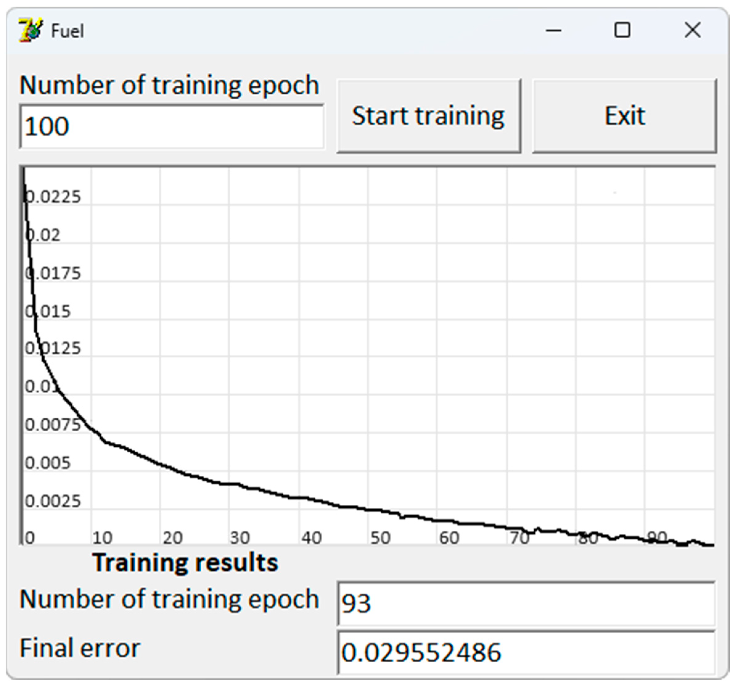
The proposed neuro-fuzzy HTE ACS in the form of a six-layer NFN AFNN is implemented in software in the Borland Delphi 7 environment and tested using the example of GT fuel consumption control according to the following input variables: nTC, , nFT. The output variable was the fuel consumption value GT, which was calculated as:
Figure 14 shows the AFNN NFN training diagram for testing the GT fuel consumption control model. Analysis of the simulation results allows us to conclude that the model has a sufficient accuracy degree: at epoch 93, the fuel consumption GT output value error became less than acceptable.
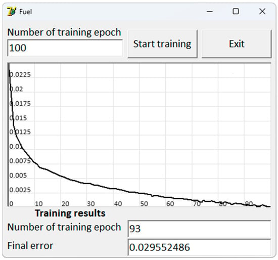
Figure 14.
Fuel consumption control model test results: OX axis represents the number of training epochs, and the OY axis represents the training error.
At the final stage of discussing the obtained results, assessment and analysis of the errors of types I and II, which are important in statistics when making statistical decisions, are carried out. The errors of type I occur when we reject a true null hypothesis. This means that a false assumption is made about the difference between the actual and model values of the controlled variable (fuel consumption parameter GT), when in fact there is no difference. The error of type I is associated with the significance level α, which defines the critical region for the test and represents the maximum acceptable probability of rejecting a true null hypothesis. The errors I type is calculated as:
When determining the controlled variable (fuel consumption parameter GT) values, the test results must show with high confidence a statistically significant difference between the actual and model values of the controlled variable (fuel consumption parameter GT); the significance level α = 0.01 was adopted in this work. This means that if the null hypothesis is true, then the probability of rejecting it (committing the error of type I) is only 1%.
Null hypothesis H0: there is no difference between the actual and the fuel consumption parameter GT model values, that is, the GT actual value is equal to the GT model value.
The error of type II occurs when we do not reject a false null hypothesis. This means that we do not detect the presence of an effect or difference when it actually exists. Type II error is related to the power of the test (1 − β), where the power of the test is the probability of correctly rejecting a false null hypothesis (or detecting an effect if one exists). Equation for the error of type II:
where the test “power” concept is defined as the probability of rejecting the null hypothesis when it is in fact false.
Table 12 shows the errors of types I and II in determining the controlled quantity (fuel consumption parameter GT) values using the proposed neuro-fuzzy HTE ACS, the basis of which is a six-layer NFN AFNN, as well as a reconfigured HTE ACS, the basis of which is a five-layer NFN ANFIS [28].

Table 12.
The type I and II calculation errors.
Thus, the use of the ANFF six-layer NFN made it possible to reduce the errors of type I by 2.06 times and the errors of type II by 1.36 times compared with the ANFIS five-layer NFN [28] as part of the neuro-fuzzy HTE ACS.
5. Conclusions
The scientific novelty of the obtained results lies in the development of the helicopter TE modified onboard neuro-fuzzy adaptive ACS, featuring a framework consisting of the research object, regulator, emulator, compensator, and observer block. Each component of this framework utilizes the proposed six-layer hybrid neuro-fuzzy network of the AFNN type, with Sugeno fuzzy inference and bell-shaped membership functions for fuzzy variables.
The NFA closed onboard TE ACS has been improved, which, by introducing an observer unit, taking into account dynamic changes in external conditions, and additional errors (noise), allows us to fulfill the task of controlling the TE fuel consumption.
In contrast to the well-known neuro-fuzzy TE ACS, which is based on an ANFIS five-layer hybrid NFN, it is proposed to use an AFNN six-layer hybrid NFN with Sugeno fuzzy inference and a fuzzy-variables bell-shaped membership function, which made it possible to reduce the HTE fuel consumption parameter transient process regulation time by 15.0 times compared with the use of a traditional ACS (precise control), by 17.5 times compared with the use of a fuzzy ACS (fuzzy control), and by 11.25 times compared with the use of neural fuzzy reconfigured ACS based on an ANFIS five-layer hybrid NFN.
The AFNN six-layer hybrid NFN training algorithm has been further developed, which, due to adaptive elements, allows us to change its parameters and settings in real time based on changing conditions or external influences and, as a result, achieve an accuracy of up to 99.98% in the TE fuel consumption controlling task and reduce losses to 0.2%.
It has been experimentally proven that the use of adaptive elements in the AFNN six-layer hybrid NFN proposed training algorithm has made it possible to reduce the mean square error square root values, the mean absolute error values, and the mean absolute percentage error values in determining the fuzzy-variables bell-shaped membership function parameters by 1.46…1.53 times compared with the use of an ANFIS five-layer hybrid NFN.
It has been experimentally proven that the use of the developed neuro-fuzzy TE ACS has made it possible to achieve an improvement in the fuel consumption parameter control quality in comparison with the precise control, fuzzy control, neuro-fuzzy control using a reconfigured ACS based on an ANFIS five-layer hybrid NFN, in terms of overshoot (overload), steady-state value (stationary deviation), and transition process time by 1.45…7.77 times.
The use of the ANFF six-layer NFN made it possible to reduce the I and II types of error in the TE fuel consumption controlling task by 1.36…2.06 times compared with the ANFIS five-layer NFN.
Author Contributions
Conceptualization, S.V., R.Y. and V.V.; methodology, S.V.; software, V.V.; validation, R.Y., M.B. and V.V.; formal analysis, S.V.; investigation, M.B.; resources, S.V., R.Y. and V.V.; data curation, M.B.; writing—original draft preparation, S.V., R.Y. and V.V.; writing—review and editing, S.V., R.Y. and V.V.; visualization, M.B.; supervision, S.V.; project administration, R.Y.; funding acquisition, M.B. All authors have read and agreed to the published version of the manuscript.
Funding
This research received no external funding.
Data Availability Statement
Data is contained within the article.
Acknowledgments
This research was supported by the Ministry of Internal Affairs of Ukraine “Theoretical and applied aspects of the development of the aviation sphere” under Project No. 0123U104884.
Conflicts of Interest
The authors declare no conflicts of interest.
Nomenclature
| d(i) is the additional parameter |
| y(i) is the output signal |
| u(i) is the control |
| f(•) is some nonlinear function having known orders r, s, q |
| e(i) is the control error |
| Xk is the the fuzzy set |
| μ is the membership function |
| θ is the rules number |
| α is the coefficient adjustable during network training or determined by expert input |
| J is the relative control error value |
| Jnom is the relative control error nominal value |
| φk is the coefficient that is a fairly large number |
| λ is the regularization parameter |
| g(•) is the emulator function |
| Jreg is the emulator average relative error |
| ϑ is the coefficient that regulates the influence of the adaptive multiplier |
| ηt is the current adaptive training rate |
| v(i) is a noise or disturbances vector |
| is the system state current assessment |
| A and B are the system or control matrices |
| C is the measurement matrix |
| K(i) is the observer gain matrix |
| P(i) is the state covariance error estimate |
| R is the measurement noise covariance matrix |
| μj are the initial centroids |
| is the model outputs vector before applying softmax for input x |
| is the vector k-th element |
| K is the classes number |
| q1,…, qi are the transient processes under consideration quality indicators |
| {ki}, {τi}, {Ti} are the variable system parameters (gain factors, time constants, etc.) sets |
| f1(•), …, fi(•) are the functions expressing the system quality indicators dependence on the synthesized controllers parameters |
| σ1,…, σi is the overshoot |
| treg1,…, treg_i is the subsystems transient processes regulation time |
| GT is the fuel consumption parameter |
| E(θk) is the loss function value at the current iteration |
| E(θ0) is the loss function initial value |
| Acci is the NFN (AFNN or ANFIS) accuracy on the i-th data set or with the i-th parameters variation |
| is the average accuracy value for all observations |
| n is the subsamples number. |
References
- Mao, X.; Xiang, Y. An efficient nonlinear adaptive filter algorithm based on the rectified linear unit. Digit. Signal Process. 2024, 146, 104373. [Google Scholar] [CrossRef]
- Jiang, Y.; Liu, L.; Feng, G. Fully distributed adaptive control for output consensus of uncertain discrete-time linear multi-agent systems. Automatica 2024, 162, 111531. [Google Scholar] [CrossRef]
- Liu, J. Gas path fault diagnosis of aircraft engine using HELM and transfer learning. Eng. Appl. Artif. Intell. 2022, 114, 105149. [Google Scholar] [CrossRef]
- Xu, M.; Wang, J.; Liu, J.; Li, M.; Geng, J.; Wu, Y.; Song, Z. An improved hybrid modeling method based on extreme learning machine for gas turbine engine. Aerosp. Sci. Technol. 2020, 107, 106333. [Google Scholar] [CrossRef]
- Montazeri-Gh, M.; Yazdani, S. Application of interval type-2 fuzzy logic systems to gas turbine fault diagnosis. Appl. Soft Comput. 2020, 96, 106703. [Google Scholar] [CrossRef]
- Sarwar, U.; Muhammad, M.; Mokhtar, A.A.; Khan, R.; Behrani, P.; Kaka, S. Hybrid intelligence for enhanced fault detection and diagnosis for industrial gas turbine engine. Results Eng. 2024, 21, 101841. [Google Scholar] [CrossRef]
- Yazdani, S.; Montazeri-Gh, M. A novel gas turbine fault detection and identification strategy based on hybrid dimensionality reduction and uncertain rule-based fuzzy logic. Comput. Ind. 2020, 115, 103131. [Google Scholar] [CrossRef]
- Djeddi, C.; Hafaifa, A.; Iratni, A.; Hadroug, N.; Chen, X. Robust diagnosis with high protection to gas turbine failures identification based on a fuzzy neuro inference monitoring approach. J. Manuf. Syst. 2021, 59, 190–213. [Google Scholar] [CrossRef]
- Gu, Z.; Li, Q.; Pang, S.; Zhou, W.; Wu, J.; Zhang, C. Turbo-shaft engine adaptive neural network control based on nonlinear state space equation. Chin. J. Aeronaut. 2024, 37, 493–507. [Google Scholar] [CrossRef]
- Baranovskyi, D.; Myamlin, S.; Kebal, I. Increasing the Carrying Capacity of the Solid-Body Rail Freight Car. Adv. Sci. Technol. Res. J. 2022, 16, 219–225. [Google Scholar] [CrossRef]
- Tereikovskyi, I.; Hu, Z.; Chernyshev, D.; Tereikovska, L.; Korystin, O.; Tereikovskyi, O. The Method of Semantic Image Segmentation Using Neural Networks. Int. J. Image Graph. Signal Process. 2022, 14, 1–14. [Google Scholar] [CrossRef]
- Vladov, S.; Yakovliev, R.; Hubachov, O.; Rud, J.; Stushchanskyi, Y. Neural Network Modeling of Helicopters Turboshaft Engines at Flight Modes Using an Approach Based on “Black Box” Models. CEUR Workshop Proc. 2024, 3624, 116–135. [Google Scholar]
- Baranovskyi, D.; Myamlin, S. The criterion of development of processes of the self organization of subsystems of the second level in tribosystems of diesel engine. Sci. Rep. 2023, 13, 5736. [Google Scholar] [CrossRef]
- Baranovskyi, D.; Bulakh, M.; Michajłyszyn, A.; Myamlin, S.; Muradian, L. Determination of the Risk of Failures of Locomotive Diesel Engines in Maintenance. Energies 2023, 16, 4995. [Google Scholar] [CrossRef]
- Baranovskyi, D.; Myamlin, S.; Podosonov, D.; Muradian, L. Determination of the filler concentration of the composite material to reduce the wear of the central bowl of the rail truck bolster. Ain Shams Eng. J. 2023, 12, 102232. [Google Scholar] [CrossRef]
- Baranovskyi, D.; Bulakh, M.; Myamlin, S.; Kebal, I. New Design of the Hatch Cover to Increase the Carrying Capacity of the Gondola Car. Adv. Sci. Technol. Res. J. 2022, 16, 186–191. [Google Scholar] [CrossRef]
- Rusyn, B.; Lutsyk, O.; Kosarevych, R.; Maksymyuk, T.; Gazda, J. Features extraction from multi-spectral remote sensing images based on multi-threshold binarization. Sci. Rep. 2023, 13, 19655. [Google Scholar] [CrossRef] [PubMed]
- Kosarevych, R.; Lutsyk, O.; Rusyn, B. Detection of pixels corrupted by impulse noise using random point patterns, The Visual Computer. Int. J. Comput. Graph. 2022, 38, 3719–3730. [Google Scholar] [CrossRef]
- Bulakh, M.; Klich, L.; Baranovska, O.; Baida, A.; Myamlin, S. Reducing Traction Energy Consumption with a Decrease in the Weight of an All-Metal Gondola Car. Energies 2023, 16, 6733. [Google Scholar] [CrossRef]
- Salilew, W.M.; Abdul Karim, Z.A.; Lemma, T.A. Investigation of fault detection and isolation accuracy of different Machine learning techniques with different data processing methods for gas turbine. Alex. Eng. J. 2022, 61, 12635–12651. [Google Scholar] [CrossRef]
- Hashmi, M.B.; Mansouri, M.; Assadi, M. Dynamic performance and control strategies of micro gas turbines: State-of-the-art review, methods, and technologies. Energy Convers. Manag. X 2023, 18, 100376. [Google Scholar] [CrossRef]
- Kilic, U.; Villareal-Valderrama, F.; Ayar, M.; Ekici, S.; Amezquita-Brooks, L.; Hikmet Karakoc, T. Deep learning-based forecasting modeling of micro gas turbine performance projection: An experimental approach. Eng. Appl. Artif. Intell. 2024, 130, 107769. [Google Scholar] [CrossRef]
- Chen, Q.; Sheng, H.; Liu, T. Fuzzy logic-based adaptive tracking weight-tuned direct performance predictive control method of aero-engine. Aerosp. Sci. Technol. 2023, 140, 108494. [Google Scholar] [CrossRef]
- Baranovskyi, D.; Myamlin, S.; Bulakh, M.; Podosonov, D.; Muradian, L. Determination of the Filler Concentration of the Composite Tape. Appl. Sci. 2022, 12, 11044. [Google Scholar] [CrossRef]
- Feng, H.; Liu, B.; Xu, M.; Li, M.; Song, Z. Model-based deduction learning control: A novel method for optimizing gas turbine engine afterburner transient. Energy 2024, 292, 130512. [Google Scholar] [CrossRef]
- Vladov, S.; Shmelov, Y.; Yakovliev, R. Helicopters Aircraft Engines Self-Organizing Neural Network Automatic Control System. CEUR Workshop Proc. 2022, 3137, 28–47. [Google Scholar] [CrossRef]
- Vladov, S.; Shmelov, Y.; Yakovliev, R.; Petchenko, M. Neural Network Method for Parametric Adaptation Helicopters Turboshaft Engines On-Board Automatic Control System Parameters. CEUR Workshop Proc. 2023, 3403, 179–195. [Google Scholar]
- Vladov, S.; Shmelov, Y.; Yakovliev, R.; Kozlovskaya, T.; Petchenko, M. Helicopters Turboshaft Engines Intelligent Control Algorithms Synthesis, Taking into Account Required Quality Provision. CEUR Workshop Proc. 2023, 3468, 71–90. [Google Scholar]
- Siddikov, I.X.; Umurzakova, D.M. Synthesis of adaptive neuro-fuzzy control system of nonlinear dynamic objects. Railw. Transp. Top. Issues Innov. 2019, 1–2, 54–73. [Google Scholar]
- Sheng, H.; Chen, Q.; Li, J.; Jiang, W.; Wang, Z.; Liu, Z.; Zhang, T.; Liu, Y. Research on dynamic modeling and performance analysis of helicopter turboshaft engine’s start-up process. Aerosp. Sci. Technol. 2020, 106, 106097. [Google Scholar] [CrossRef]
- Turan, Ö.; Aydın, H. Numerical calculation of energy and exergy flows of a turboshaft engine for power generation and helicopter applications. Energy 2016, 115, 914–923. [Google Scholar] [CrossRef]
- Togni, G.; Nikolaidis, T.; Sampath, D. A combined technique of Kalman filter, artificial neural network and fuzzy logic for gas turbines and signal fault isolation. Chin. J. Aeronaut. 2021, 34, 124–135. [Google Scholar] [CrossRef]
- Pasieka, M.; Grzesik, N.; Kuźma, K. Simulation modeling of fuzzy logic controller for aircraft engines. Int. J. Comput. 2017, 16, 27–33. [Google Scholar] [CrossRef]
- Gao, J.; Heng, F.; Yuan, Y.; Liu, Y. A novel machine learning method for multiaxial fatigue life prediction: Improved adaptive neuro-fuzzy inference system. Int. J. Fatigue 2024, 178, 108007. [Google Scholar] [CrossRef]
- Shihabudheen, K.V.; Pillai, G.N. Recent advances in neuro-fuzzy system: A survey. Knowl.-Based Syst. 2018, 152, 136–162. [Google Scholar] [CrossRef]
- Gudla, S.; Rao, K.N. Reliable Data Delivery Using Fuzzy Reinforcement Learning in Wireless Sensor Networks. Int. J. Comput. Netw. Inf. Secur. 2023, 15, 96–107. [Google Scholar] [CrossRef]
- Chang, Q.; Zhang, Z.; Wei, F.; Wang, J.; Pedrycz, W.; Pal, N.R. Adaptive Nonstationary Fuzzy Neural Network. Knowl.-Based Syst. 2024, 288, 111398. [Google Scholar] [CrossRef]
- Zhang, Y.; Wang, G.; Huang, X.; Ding, W. TSK fuzzy system fusion at sensitivity-ensemble-level for imbalanced data classification. Inf. Fusion 2023, 92, 350–362. [Google Scholar] [CrossRef]
- Vladov, S.; Yakovliev, R.; Hubachov, O.; Rud, J. Neuro-Fuzzy System for Detection Fuel Consumption of Helicopters Turboshaft Engines. CEUR Workshop Proc. 2023, 3628, 628–647. [Google Scholar]
- Marakhimov, A.R.; Khudaybergenov, K.K. Approach to the synthesis of neural network structure during classification. Int. J. Comput. 2020, 19, 20–26. [Google Scholar] [CrossRef]
- Hu, Z.; Buriachok, V.; TajDini, M.; Sokolov, V. Authentication System by Human Brainwaves Using Machine Learning and Artificial Intelligence. Lect. Notes Data Eng. Commun. Technol. 2021, 83, 374–388. [Google Scholar] [CrossRef]
- Liu, J.; Zhao, T.; Cao, J.; Li, P. Interval type-2 fuzzy neural networks with asymmetric MFs based on the twice optimization algorithm for nonlinear system identification. Inf. Sci. 2023, 929, 123–143. [Google Scholar] [CrossRef]
- Xu, D.; Zhang, S.; Zhang, H.; Mandic, D.P. Convergence of the RMSProp deep learning method with penalty for nonconvex optimization. Neural Netw. 2021, 139, 17–23. [Google Scholar] [CrossRef]
- Barrau, A.; Bonnabel, S. Three examples of the stability properties of the invariant extended Kalman filter. IFAC-PapersOnLine 2017, 50, 431–437. [Google Scholar] [CrossRef]
- Vladov, S.; Yakovliev, R.; Bulakh, M.; Vysotska, V. Neural Network Approximation of Helicopter Turboshaft Engine Parameters for Improved Efficiency. Energies 2024, 17, 2233. [Google Scholar] [CrossRef]
- Vladov, S.; Petchenko, M.; Shmelov, Y.; Drozdova, S.; Yakovliev, R. Helicopters Turboshaft Engines Parameters Identification at Flight Modes Using Neural Networks. In Proceedings of the 2022 IEEE 17th International Conference on Computer Sciences and Information Technologies (CSIT), Lviv, Ukraine, 10–12 November 2022. [Google Scholar] [CrossRef]
- Vladov, S.; Scislo, L.; Sokurenko, V.; Muzychuk, O.; Vysotska, V.; Osadchy, S.; Sachenko, A. Neural Network Signals Integration from Thermogas-dynamic Parameters Sensors for Helicopters Turboshaft Engines at Flight Operation Conditions. Sensors 2024, 24, 4246. [Google Scholar] [CrossRef] [PubMed]
- Corotto, F.S. Appendix C—The method attributed to Neyman and Pearson. In Wise Use of Null Hypothesis Tests; Academic Press: Cambridge, MA, USA, 2023; pp. 179–188. [Google Scholar] [CrossRef]
- Motsnyi, F.V. Analysis of Nonparametric and Parametric Criteria for Statistical Hypotheses Testing. Chapter 1. Agreement Criteria of Pearson and Kolmogorov. Stat. Ukr. 2018, 83, 14–24. [Google Scholar] [CrossRef]
- Babichev, S.; Krejci, J.; Bicanek, J.; Lytvynenko, V. Gene expression sequences clustering based on the internal and external clustering quality criteria. In Proceedings of the 2017 12th International Scientific and Technical Conference on Computer Sciences and Information Technologies (CSIT), Lviv, Ukraine, 5–8 September 2017. [Google Scholar] [CrossRef]
- Hu, Z.; Kashyap, E.; Tyshchenko, O.K. GEOCLUS: A Fuzzy-Based Learning Algorithm for Clustering Expression Datasets. Lect. Notes Data Eng. Commun. Technol. 2022, 134, 337–349. [Google Scholar] [CrossRef]
- Centorrino, V.; Bullo, F.; Russo, G. Modeling and contractivity of neural-synaptic networks with Hebbian learning. Automatica 2024, 164, 111636. [Google Scholar] [CrossRef]
- Wang, Y.; Wang, Z. Model free adaptive fault-tolerant tracking control for a class of discrete-time systems. Neurocomputing 2020, 412, 143–151. [Google Scholar] [CrossRef]
- Anfilets, S.; Bezobrazov, S.; Golovko, V.; Sachenko, A.; Komar, M.; Dolny, R.; Kasyanik, V.; Bykovyy, P.; Mikhno, E.; Osolinskyi, O. Deep multilayer neural network for predicting the winner of football matches. Int. J. Comput. 2020, 19, 70–77. [Google Scholar] [CrossRef]
- Andriushchenko, K.; Rudyk, V.; Riabchenko, O.; Kachynska, M.; Marynenko, N.; Shergina, L.; Kovtun, V.; Tepliuk, M.; Zhemba, A.; Kuchai, O. Processes of managing information infrastructure of a digital enterprise in the framework of the «Industry 4.0» concept. East.-Eur. J. Enterp. Technol. 2019, 1, 60–72. [Google Scholar] [CrossRef]
- Vladov, S.; Yakovliev, R.; Vysotska, V.; Nazarkevych, M.; Lytvyn, V. The Method of Restoring Lost Information from Sensors Based on Auto-Associative Neural Networks. Appl. Syst. Innov. 2024, 7, 53. [Google Scholar] [CrossRef]
- Vladov, S.; Yakovliev, R.; Hubachov, O.; Rud, J.; Drodova, S.; Perekrest, A. Modified Discrete Neural Network PID Controller for Controlling the Helicopters Turboshaft Engines Free Turbine Speed. In Proceedings of the 2023 IEEE 5th International Conference on Modern Electrical and Energy System (MEES), Kremenchuk, Ukraine, 27–30 September 2023; pp. 797–802. [Google Scholar] [CrossRef]
- Kovtun, V.; Altameem, T.; Al-Maitah, M.; Kempa, W. Simple Statistical Tests Selection Based Parallel Computating Method Ensures the Guaranteed Global Extremum Identification. J. King Saud Univ.–Sci. 2024, 36, 103165. [Google Scholar] [CrossRef]
Disclaimer/Publisher’s Note: The statements, opinions and data contained in all publications are solely those of the individual author(s) and contributor(s) and not of MDPI and/or the editor(s). MDPI and/or the editor(s) disclaim responsibility for any injury to people or property resulting from any ideas, methods, instructions or products referred to in the content. |
© 2024 by the authors. Licensee MDPI, Basel, Switzerland. This article is an open access article distributed under the terms and conditions of the Creative Commons Attribution (CC BY) license (https://creativecommons.org/licenses/by/4.0/).

