Article

A Deep Learning Quantile Regression Photovoltaic Power-Forecasting Method under a Priori Knowledge Injection

1
School of Renewable Energy, North China Electric Power University, Beijing 102206, China
2
School of Automation and Electrical Engineering, Inner Mongolia University of Science and Technology, Baotou 014010, China
3
Inner Mongolia Huadian New Energy Co., Hohhot 010090, China
*
Author to whom correspondence should be addressed.
Energies 2024, 17(16), 4026; https://doi.org/10.3390/en17164026
Submission received: 20 July 2024 / Revised: 4 August 2024 / Accepted: 7 August 2024 / Published: 14 August 2024
(This article belongs to the Section A2: Solar Energy and Photovoltaic Systems)

Abstract

:
Accurate and reliable PV power probabilistic-forecasting results can help grid operators and market participants better understand and cope with PV energy volatility and uncertainty and improve the efficiency of energy dispatch and operation, which plays an important role in application scenarios such as power market trading, risk management, and grid scheduling. In this paper, an innovative deep learning quantile regression ultra-short-term PV power-forecasting method is proposed. This method employs a two-branch deep learning architecture to forecast the conditional quantile of PV power; one branch is a QR-based stacked conventional convolutional neural network (QR_CNN), and the other is a QR-based temporal convolutional network (QR_TCN). The stacked CNN is used to focus on learning short-term local dependencies in PV power sequences, and the TCN is used to learn long-term temporal constraints between multi-feature data. These two branches extract different features from input data with different prior knowledge. By jointly training the two branches, the model is able to learn the probability distribution of PV power and obtain discrete conditional quantile forecasts of PV power in the ultra-short term. Then, based on these conditional quantile forecasts, a kernel density estimation method is used to estimate the PV power probability density function. The proposed method innovatively employs two ways of a priori knowledge injection: constructing a differential sequence of historical power as an input feature to provide more information about the ultrashort-term dynamics of the PV power and, at the same time, dividing it, together with all the other features, into two sets of inputs that contain different a priori features according to the demand of the forecasting task; and the dual-branching model architecture is designed to deeply match the data of the two sets of input features to the corresponding branching model computational mechanisms. The two a priori knowledge injection methods provide more effective features for the model and improve the forecasting performance and understandability of the model. The performance of the proposed model in point forecasting, interval forecasting, and probabilistic forecasting is comprehensively evaluated through the case of a real PV plant. The experimental results show that the proposed model performs well on the task of ultra-short-term PV power probabilistic forecasting and outperforms other state-of-the-art deep learning models in the field combined with QR. The proposed method in this paper can provide technical support for application scenarios such as energy scheduling, market trading, and risk management on the ultra-short-term time scale of the power system.

1. Introduction

1.1. Motivation

Solar photovoltaic (PV) power generation, as one of the important clean energy sources, has been developing rapidly in recent years. The latest data from the International Energy Agency (IEA) show that in 2022, solar photovoltaic (PV) power generation increased by a record 270 terawatt-hours (a 26% increase), and solar PV power generation had the largest absolute growth in power generation among all renewable energy technologies. In 2023, solar PV alone accounted for three-quarters of the world’s renewable energy power generation additions, and over the next five years, renewable energy power-generation capacity additions will continue to increase, with solar PV and wind power accounting for a record 96% [1]. While the rapid and large-scale penetration of PV energy in the power grid, its own fluctuations and uncertainties pose further challenges to the safe and economic dispatch and operation of the grid. Accurate PV power forecasting can be an important technical support to help optimize power system scheduling and operation, enable renewable energy integration and dispatch, support power markets and energy trading, and guide grid planning and investment decisions.
Traditional deterministic PV power forecasts give only a definite forecast value for each point in time, ignoring other aspects of the data distribution, such as different levels of variability and tail behavior, and failing to quantify such uncertainties [2]. In contrast, probabilistic forecasting provides information on the probabilistic distribution of PV power, through which grid operators and market participants can assess forecast uncertainty and make more informed decisions [3]. For example, in terms of energy scheduling and operation optimization, grid operators can rationally arrange and adjust energy supply methods to cope with PV energy fluctuations based on the information of probability distributions; in terms of risk assessment and decision support, for impending higher PV power fluctuations, system operators can take appropriate measures to ensure the stable operation of the power system; in terms of real-time monitoring and anomaly detection, operators can detect possible system anomalies (e.g., module failure, shadow coverage, etc.) based on the expected range of actual power deviation from the predicted probability distribution to avoid system performance degradation or failures; in terms of power market transactions, market participants can formulate power purchasing and selling strategies based on power probability prediction results to maximize profits.
In conclusion, accurate PV power probabilistic forecasting helps to improve the reliability, stability, and economy of the power system and is one of the important technical means in the process of clean energy transition.

1.2. Related Works

PV power probabilistic-forecasting techniques have received increasing attention for quantifying PV power uncertainty. The development of PV power probabilistic-forecasting techniques has gone through several stages, from traditional statistical methods to machine learning (ML) and deep learning (DL)-based methods, and these variations are mainly aimed at improving forecast accuracy, adapting to complex PV power systems and data characteristics, and meeting the growing demand for renewable energy. PV power probabilistic-forecasting methods can be mainly categorized into parametric and non-parametric-based methods. Parametric methods assume that the probability distribution of PV power belongs to some known parametric distribution, such as Gaussian distribution [4], gamma distribution [5], and beta distribution [6,7]. These methods estimate parameters from historical data and then utilize the parameter distributions for probabilistic forecasting. Commonly used methods include maximum likelihood estimation and Bayesian estimation [8]. These methods have the advantage of high computational efficiency, but the assumptions on the power distribution depend heavily on the distribution of the data and may not accurately reflect the true power distribution. Non-parametric methods are insensitive to the distribution of historical data and do not make specific assumptions about the probability distribution of PV power but make probabilistic forecasts by directly modeling the distribution of historical data.
Current research on PV power probabilistic-forecasting techniques focuses on non-parametric methods (e.g., quantile regression (QR) [9] and kernel density estimation (KDE) [10]). These methods usually utilize the QR method to obtain power-forecasting results at different quantiles. These quantiles can represent different probability levels. By estimating the regression coefficients for different quartiles, the power forecast at different probability levels can be obtained. Then, the probability density function (PDF) is estimated by techniques such as KDE and histogram, and finally the probabilistic forecast is calculated based on the probability density function. Compared with parametric methods, non-parametric methods are more flexible and applicable to data with different distribution patterns, and they can provide more comprehensive probability forecasting results, including the predicted values and confidence intervals estimated under different probability levels. Current research has focused on probabilistic-forecasting methods that combine QR with ML. ML methods (e.g., Support Vector Machine Regression (SVR) [11], Random Forest [12], Artificial Neural Networks (ANN) [13], etc.) can solve the nonlinear regression problem better and improve the forecasting performance more significantly compared with statistical methods [14]. Among them, DL methods, as a branch of ML, are able to capture complex nonlinear relationships due to their deep structure and nonlinear activation function and show better feature learning ability than the above traditional ML methods for nonlinear and nonsmooth time series data such as photovoltaic power, and are therefore applied to the research field of probabilistic forecasting of PV power [15]. The DL models with relatively more applications in the field are Recurrent Neural Networks (RNNs), Long Short-Term Memory Networks (LSTMs), Gated Recurrent Units (GRUs), and Convolutional Neural Networks (CNNs) [16]. By integrating the QR method into the DL model, the DL architecture can forecast multiple quantiles at the same time by sharing the underlying representation, realizing multi-task learning, and improving the consistency and efficiency of forecasting. The DL probabilistic-forecasting method based on the QR method provides a probabilistic framework for PV power forecasting and is therefore increasingly used in PV power probabilistic-forecasting application scenarios. A QRLSTM-based day-ahead PV power-forecasting method is proposed in the literature [17]. Firstly, the PV power feature is reconstructed by the K-means clustering algorithm and deep convolutional generative adversarial network (GAN) [18] model, and then this feature and other explanatory variables are used as inputs to the QRLSTM model to obtain the PV power-forecasting results and the prediction intervals at different confidence levels. The experimental results show that the forecasting performance of the proposed method has obvious advantages over the Gaussian Process Regression (GPR) model and the single QRLSTM model, respectively. Literature [19] presents a PV power probabilistic-forecasting method based on a Coupled Input and Forgotten Gate (CIFG) network in combination with QR. Maximum information coefficient (MIC) is used to select the feature variables. QR combined with CIFG is used to forecast the quantile of PV power, and KDE is used to estimate the PDF of the PV output. Comparison with QRLSTM, QRGRU, and QRRNN demonstrates the effectiveness of the model. A hybrid deterministic and probabilistic PV power-forecasting method based on wavelet transform (WT) and deep convolutional neural network (DCNN) is proposed in the literature [20]. WT is used to decompose the original signal into multiple frequency sequences. DCNN is used to extract the nonlinear features and invariant structure of each frequency. Then, the proposed deterministic forecasting method is combined with spine QR to build a probabilistic PV power-forecasting model, which achieves better forecasting results when compared with the ML models support vector machine (SVM) [21] and back-propagation neural network (BPNN). The literature [22] proposes a probabilistic-forecasting method for day-ahead PV power based on improved QR_CNN. A two-stage training strategy is used to train the CNN and QR, respectively, which achieves better forecasting results compared to quantile limit learning machine, QR, and radial basis function neural network. Literature [23] fuses CNN and LSTM as a forecasting model and performs PV power probability interval forecasting using QR and KDE, verifying the reliability of the results.
Temporal Convolutional Networks (TCNs) [24] are a DL model specialized in processing time series data. The main characteristic of TCN is the use of causal convolutions and dilated convolutions combined with residual connections. These characteristics allow TCNs to capture patterns over a long time span while maintaining computational efficiency. As a relatively new DL model, TCN has begun to be applied in the field of deterministic PV power forecasting [25,26,27] and has demonstrated its advantages in improving forecasting accuracy and handling complex data patterns. However, few studies have combined it with QR to perform probabilistic-forecasting tasks.

1.3. The Research Work in This Paper

In the above literature study, it can be seen that the QR-based DL PV power probabilistic-forecasting technique gives better forecasting results than the traditional parametric and ML-based methods. The research mainly focuses on two aspects: in terms of input feature engineering, most of them decompose the PV power data into different sub-sequences or modal components in order to provide the model with information of different time scales or frequency ranges. Alternatively, the input features are selected based on relevance, and the introduction of a priori features combined with forecasting scenarios and multi-input feature combination approaches are rarely seen; in terms of the selection of QR-based DL models, the studies have focused on the application of classical RNN, LSTM, GRU, and CNN, and very few studies have been conducted on the application of combining TCNs and QR to the task of probabilistic PV power forecasting. Inspired by the above studies, this study proposes a novel QR probabilistic-forecasting model based on deep convolutional architecture under a priori knowledge injection from the perspectives of input feature engineering and deep model selection and architecture design and applies it to the task of ultra-short-term probabilistic forecasting of PV power. The specific contributions of this study are as follows:
(1)
Model QR_CNN-TCN is proposed to be applied to the task of ultra-short-term PV power probabilistic forecasting. TCN is innovatively introduced into the field of PV power probabilistic forecasting, and the dilation and causal convolution structure of TCN is utilized to obtain the long-time dependencies among the elements of the input feature sequence.
(2)
Combined with the ultra-short-term PV power-forecasting application scenario, the PV power first-order differential sequence is innovatively introduced as an input feature, and all the input data are divided into two groups of input feature data containing different prior knowledge to provide dual-channel inputs to the model.
(3)
Innovatively integrating domain a priori knowledge into the model architecture design and deeply matching the input feature data with the model-computing mechanism, two-branch DL networks (CNN-TCN) with different convolutional structures are designed to extract finer and diversified feature information at different spatial and temporal scales from the two input channels, respectively.
(4)
The QR method is combined with DL architecture (CNN-TCN) to give full play to the advantages of DL multi-task learning to obtain the power forecasts under different probability levels, and the KDE estimates the PDF of the forecasting results and finally realizes the point forecasting, interval forecasting, and probabilistic forecasting of PV power.
(5)
Comparing with the current state-of-the-art DL model combined with QR, the experimental results show that the point-forecasting accuracy of the proposed method is the highest among all the models, the obtained prediction intervals are the most reasonable, and the comprehensive performance of the obtained probabilistic-forecasting results is also optimal. Meanwhile, the good applicability of the proposed model is verified on three different PV plant datasets.
The rest of the research in this paper is organized as follows: Section 2 provides a detailed description of the basic models and related theories involved in this study. Section 3 provides a detailed introduction to the performance evaluation indexes for point, interval, and probabilistic forecasting used in this paper. Section 4 provides a detailed presentation and analysis of the experiments related to the various forecasting tasks performed in this study. Section 5 summarizes and discusses the overall study in this paper.

2. Methodology

This section first describes the QR method and its rationale for combining it with the DL point-forecasting methods (CNN and TCN) used in this study. Then, a novel DL PV power-forecasting model combining QR methods is proposed and elaborated. Finally, the KDE method and its details of post-processing the discrete multi-quantile forecasting results are presented. The overall research flowchart of the proposed method in this paper is shown in Figure 1.

2.1. Quantile Regression

The QR method, first proposed by Roger Koenker and Gilbert Bassett, is a typical nonparametric probabilistic-forecasting model. The method overcomes the limitation that traditional linear regression models only provide information about the mean and ignore the distribution of the data and is used to estimate the relationship between different quantiles of the dependent variable and the independent variable. By estimating the conditional distributions of different quantiles, QR can reveal richer distributional information about the data, especially when the data do not conform to normal distribution or there are outliers, which is very favorable for PV system data. The mathematical expression of QR is as follows:
Q ( τ | X ) = X β ( τ )
where Q ( τ | X ) is the conditional τ quantile given the explanatory variables X , X is a matrix of explanatory variables, and β ( τ ) is the quantile regression coefficients, which is a vector whose elements are the coefficients for each explanatory variable. For each τ , there is a linear model that predicts the corresponding quantile. The regression coefficient β ( τ ) is obtained by minimizing the quantile loss function L . The mathematical expression for L is given below:
L = t = 1 n ρ τ ( y t x t Τ β )
where ρ τ is the quantile loss function for each observation, defined as
ρ τ ( u ) = u ( τ I ( u < 0 ) )
where u = y t x t Τ β is the residual, and I is an indicator function with a value of 1 when u < 0, and 0 otherwise. Essentially, ρ τ is a weighted absolute value loss with weights determined by τ .

2.2. The 1D CNN and TCN

The 1D CNN has been widely used in the field of time series forecasting. It has the advantages of efficient local feature extraction, high computational efficiency, and parameter sharing. Usually, 1D CNN architectures contain pooling layers and activation functions, which further enhance its performance and application scope. Convolutional operations extract localized time-dependent features from the time series and can effectively capture the short-term dependence of the data, which is ideal for PV power-forecasting tasks on ultra-short-term time scales. The convolution kernel shares parameters at different locations in the time series, which reduces the number of parameters in the model and makes 1D CNNs faster to train compared to recurrent class neural networks. The pooling layer is usually located behind the convolution layer and is used to reduce the spatial dimensionality of the data while retaining the most important features. There are various pooling operations, such as Max Pooling, Average Pooling, Global Max Pooling and Global Average Pooling. The appropriate pooling method can be selected according to the specific application task. Pooling reduces the computational burden while helping to make the feature detector more invariant and improve the generalization ability of the model. Activation functions such as ReLU (Rectified Linear Unit) are used to introduce nonlinearity, which is the key to solving nonlinear problems and allowing the network to learn more complex patterns. The mathematical expression for the feature map of a 1D CNN at each time step in the point-forecasting task [28] is as follows:
Y t = σ ( W t X t + b t )
where Y t is the output feature map when each convolutional kernel is slid by 1 step, W t is the weight matrix of the filter, X t is the input feature map under the field of view of the convolutional kernel, b t is the bias term, and σ is the activation function.
If the 1D CNN is combined with the QR method to perform the forecasting task, i.e., when the loss function of the model is Equation (3), the mathematical expression of the estimated output feature map of the 1D CNN for each time step is
Y ^ t ( τ ) = σ ( W t ( τ ) X t + b t ( τ ) )
That is, for different quantiles, the model has a set of parameters corresponding to them. Assuming that in the point-forecasting task, the output function of the convolution after the pooling layer is f ^ c n n ( x t , Ω ^ c n n ) , where Ω ^ c n n represents all the parameters to be learned by the model and x t represents the input features of the model, the output function can be expressed as f ^ c n n ( x t , Ω ^ c n n ( τ ) ) after combining it with the QR method. With this combination, 1D CNNs can be optimized directly for the forecasting of the different quartiles, thus capturing the short-term localized complex patterns of the time series while providing detailed insight into different parts of the data distribution.
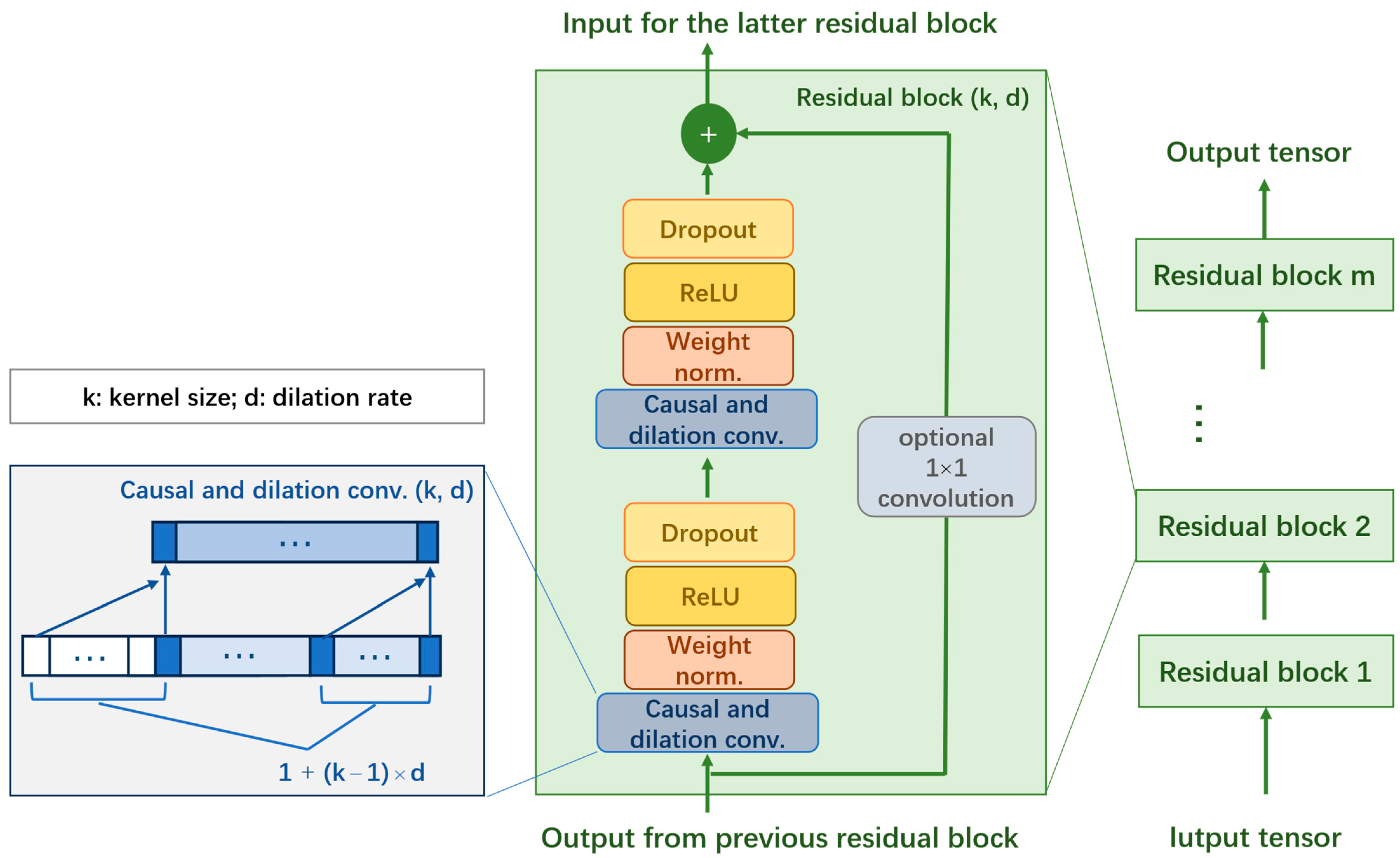
The 1D CNN mainly focuses on local features and has limited ability to capture long-range dependencies and requires multi-layer convolution to expand the receptive field, but it will increase the model complexity and training difficulty. Therefore, this study introduces TCN into the overall model architecture. TCN can be regarded as a variant of 1D CNN, which is specially designed for processing time series data. TCN adds causal convolution, dilation convolution, and residual connection on the basis of 1D CNN. The model structure diagram of TCN is shown in Figure 2.
Causal convolution ensures that the output time step t depends only on the current and previous time steps, preventing future information from leaking into the current forecast. The dilation convolution uses a dilation rate to perform the convolution operation, allowing the network to see a larger time window at each hidden layer, effectively capturing long time dependencies without increasing the number of parameters. The residual connection can be thought of as an “in-network shortcut”, where the inputs of the layer (which are linearly transformed to make the dimensions match) are added to the output to obtain a residual block of outputs. This operation improves training speed and stability while ensuring that historical information is propagated and utilized in the network. The output expression of the single-layer TCN structure is as follows:
y t = ( F d X ) ( x t ) = k = 1 K f k x t ( K k ) d
where X = ( x 1 , x 2 , , x n ) is the input sequence, W = ( w 1 , w 2 , , w K ) is the filter, and F d X represents a convolution operation with an expansion rate of d .
The introduction of these three structures results in superior performance of TCN on the task of capturing long-term dependencies. In this study, the QR method is innovatively combined with the TCN to capture the long-term dependencies between the elements of the PV power sequence at different quantiles, thus indirectly providing different parts of the PV power distribution. Assuming that the final output of the TCN is f ^ t c n ( x t , Ω ^ t c n ) , as in the case of the 1D CNN, its output function can be expressed as f ^ t c n ( x t , Ω ^ t c n ( τ ) ) when combined with QR.

2.3. Proposed QR-Based DL Probabilistic-Forecasting Architecture

In this study, we inject domain a priori knowledge into the DL model and utilize the multilayer processing units (neurons) and nonlinear activation functions of the DL model to build a complex nonlinear mapping. We combine the QR method with the DL architecture and finally form a nonlinear quantile regression model—QR_CNN-TCN. The whole model architecture and forecasting flow is shown in Figure 3.
First, this study innovatively constructs a first-order difference sequence of PV historical power as a new input feature to provide the model with a priori dynamic trends between neighboring elements of historical power.
Then, this study incorporates the a priori knowledge into the model architecture design and matches the input features to the network by utilizing the different feature-extraction mechanisms of the two DL network branches. All the selected features, along with the PV power first-order difference sequences, are recombined into two sets of input feature data, which are used as inputs to the two branch networks, respectively. In this case, the historical power sequence, together with its difference sequence (Input 1 in Figure 3), is used as input to the CNN branch, which consists of two stacked layers of 1D CNNs combined with 1D Max Pooling and 1D Global Max Pooling, respectively. Several other meteorological feature sequences are used as inputs to the TCN branch along with historical power sequences (Input 2 in Figure 3). For the QR-CNN branch in the two-branch DL architecture, the short-term spatio-temporal cross-feature-extraction capability of CNN is utilized to learn the constraints among the elements of the historical power sequences at different quantiles, while for the QR_TCN branch, the long-range spatio-temporal dependencies between the target sequences and the weather variable sequences at different quantiles are learned by utilizing the dilation and causal convolutional structure of TCN.
Finally, the output feature maps of the above two branches are concatenated into one long vector using the concatenation operation, which is used as the input to the last fully connected (FC) layer. The FC layer utilizes the same number of neurons as the number of quantiles to be predicted to output the forecast results of different quantiles. The output of the whole model can be expressed as
Q ^ y t ( τ | x t ) = f ^ c n n _ t c n ( x t , Ω ^ c n n _ t c n ( τ ) )
where Ω ^ c n n _ t c n ( τ ) stands for all the parameters under different quantiles that need to be learned by the proposed model.
In the whole process of DL model learning, combined with the QR method, the DL model builds a complex nonlinear mapping through multiple layers of processing units (neurons) and nonlinear activation function (ReLU); in the process of multi-task learning, the model parameters are shared, which allows the model to transfer knowledge between different tasks, thus improving the efficiency of learning. The quantile loss function varies with the forecasting quantile and is adjusted accordingly to minimize the quantile loss; finally, a nonlinear QR model is formed to obtain interval-forecasting and deterministic-forecasting results.

2.4. Kernel Density Estimation

After forecasting the PV power using the QR-based deep learning model, N discrete PV power quantile forecast values are obtained at each time step, which can be described as q ^ t = [ Q y t ( τ 1 | x t ) , Q y t ( τ 2 | x t ) , , Q y t ( τ N | x t ) ] . τ 1 , τ 2 , , τ N are the values obtained by dividing 0 and 1 between N + 1 equal parts. However, this result does not provide a continuously smoothed power probability density function.
KDE [10], as a non-parametric method, is completely data-driven, does not require strong assumptions about the form of the distribution of the data, and can intuitively output the probabilities, which is an important advantage for complex and irregular PV power data. For the above sample of equally spaced quantile forecasting results, the expression for kernel density estimation is as follows:
f ^ ( x ) = 1 N h i = 1 N K q ^ t , i x h
where K ( ) is the kernel function. h is the bandwidth. The effect of KDE depends heavily on the choice of kernel function and the setting of bandwidth. The kernel function determines the shape of the effect of each data point on the surrounding area, while the bandwidth determines the size of the range of this effect. The correct choice of kernel function and bandwidth is essential to obtain accurate density estimates. PV power data do not usually follow a strict normal distribution due to the underlying physical processes and may contain multiple patterns and outliers. In this study, the Epanechnikov kernel [29] is used as the kernel function of the KDE. Its mathematical expression is
K ( u ) = 3 4 ( 1 u 2 ) I ( u 1 )
where I ( u 1 ) is the indicator function, which is 1 when u 1 , and 0 otherwise. Epanechnikov is a nonparametric method that does not have strict requirements on the distribution of the input data and can effectively model the non-Gaussian nature of the power output data, providing a more accurate representation of the underlying distribution than parametric methods. Its tight support property reduces the effect of outliers and density estimation is more robust [29]. In this study, a cross-validation approach [30] is used to select the bandwidths. Cross-validation allows a data-driven approach to accommodate the complexity of the PV power data, selecting the optimal bandwidths by minimizing the actual prediction error, thus providing more accurate and reliable density estimates.

3. Performance Evaluation Index

3.1. Point-Forecasting Evaluation Index

In order to comprehensively assess the performance of model point forecasting from different perspectives, three commonly used assessment indexes, namely, the mean absolute error (MAE), root mean square error (RMSE), and coefficient of determination ( R 2 ), are used in this study. The corresponding expressions are as follows:
M A E = 1 N t = 1 N p t p ^ t
R M S E = 1 N t = 1 N ( p t p ^ t ) 2
R 2 = 1 t ( p t p ^ t ) 2 t ( p t p ¯ p e r i o d ) 2
where p t is the observed value of PV power, p ^ t is the predicted value, p ¯ p e r i o d is the average of the observations over the entire forecast interval segment, and N is the number of samples on the forecast interval segment. RMSE is concerned with large errors. MAE is more intuitive and easier to interpret, is insensitive to outliers, and provides a relatively robust assessment of performance. R 2 measures the model’s ability to explain the variability in the data, which quantifies the correlation between the model’s predicted values and the actual values, and ranges in value from 0 to 1. Higher values indicate that the model is able to account for a large portion of the variability in the dependent variable, i.e., that the model captures most of the patterns and relationships in the data.

3.2. Interval Forecasting Evaluation Index

An ideal interval-forecasting model should provide both compact and accurate forecasting intervals, and this means that the forecasting intervals should be neither too wide to avoid useless forecasts nor too narrow to miss the true values. The Prediction Interval Coverage Probability (PICP) is a commonly used statistical metric for assessing the quality of prediction intervals and is used to assess the probability that an observation falls within the prediction interval, taking values between 0 and 1. Ideally, the PICP should be close to the coverage probability of the designed interval (e.g., a 95% confidence interval). A prediction interval that is too wide may have a high PICP, but this does not mean that the prediction is meaningful because it does not provide enough precise information. Therefore, the PICP is usually used in conjunction with evaluation metrics that measure the width of the prediction interval to comprehensively assess the performance of the model. The prediction interval normalized averaged width (PINAW) [31] is an evaluation metric used to calculate the average of the width of the prediction intervals for all time points, aiming at obtaining narrower intervals to improve the sharpness of the prediction. However, it does not take into account whether the observations fall within the interval or not, and only measures the average width of the prediction interval across all points, which lacks a measure of the accuracy of the interval. The Winkler score (WS) is a composite metric for evaluating prediction intervals, and is more objective in assessing the overall quality of the prediction intervals [32]. It considers both the width of the interval and the accuracy of the interval and penalizes intervals that fail to contain true values, which makes it a more comprehensive measure. A lower WS means a narrower confidence interval and less penalty for covering observations outside the interval. Therefore, in this study, PICP combined with WS is used to evaluate the interval prediction performance of the model in a comprehensive and objective way. Their mathematical expressions are as follows:
P I C P = 1 N P I i = 1 N P I a i
W S = 1 N P I i = 1 N P I δ i + 2 α ( L i y i ) , y i < L i δ i , L i y i U i δ i + 2 α ( y i U i ) , y i > U i
where N P I represents the number of prediction intervals, and a i is an indicator function. If the observation y i falls within the prediction interval L i , U i , it is 1; otherwise, it is 0. L i is the lower boundary of the prediction interval, and U i is the upper boundary. δ i corresponds to the interval prediction width for each forecast time step. α is the nominal coverage probability (e.g., α = 0.05 for 95% of the prediction intervals).

3.3. Probabilistic-Forecasting Evaluation Index

The Continuous Ranked Probability Score (CRPS) is used to measure the degree of match between the predicted probability distribution and the actual observations. The smaller the value of CRPS, the better the agreement between the forecast and the actual observations, and the more accurate the forecast [33]. Unlike point forecasts, which provide only a single predictive value, probabilistic forecasts provide probability distributions for a range of possible outcomes. CRPS focuses on the bias of the point predictions along with the shape and breadth of the forecast distributions, providing a comprehensive evaluation of the accuracy and reliability of the model. CRPS is calculated based on the Cumulative Distribution Function (CDF), which calculates the score by comparing the CDFs of the predicted values and the observed values, and its mathematical expression is as follows:
C R P S = 1 N test i = 1 N t e s t + [ F ( y ^ i ) H ( y ^ i y i ) ] 2 d y ^ i
where N t e s t represents the number of samples in the test set, F ( y ^ i ) represents the CDF of the predicted values, and H ( y ^ i y i ) is a unit step function that is 0 when the predicted value is less than the observed value, and 1 otherwise.

4. Case Study

4.1. Experimental Input Data

The experimental data used in this study are actual operational data from three different PV power plants located in China. These three plants have different meteorological conditions. The length of the data for each plant is one year (from 1 January 2019 to 1 January 2020). The data are collected at a temporal resolution of 15 min per sample point and all contain 35,040 sample points. The data from all three plants contain seven feature variables: power (MW), total irradiance (w/m2), normal direct irradiance (w/m2), horizontal scattered irradiance (w/m2), temperature (°C), humidity (%), and air pressure (hpa).
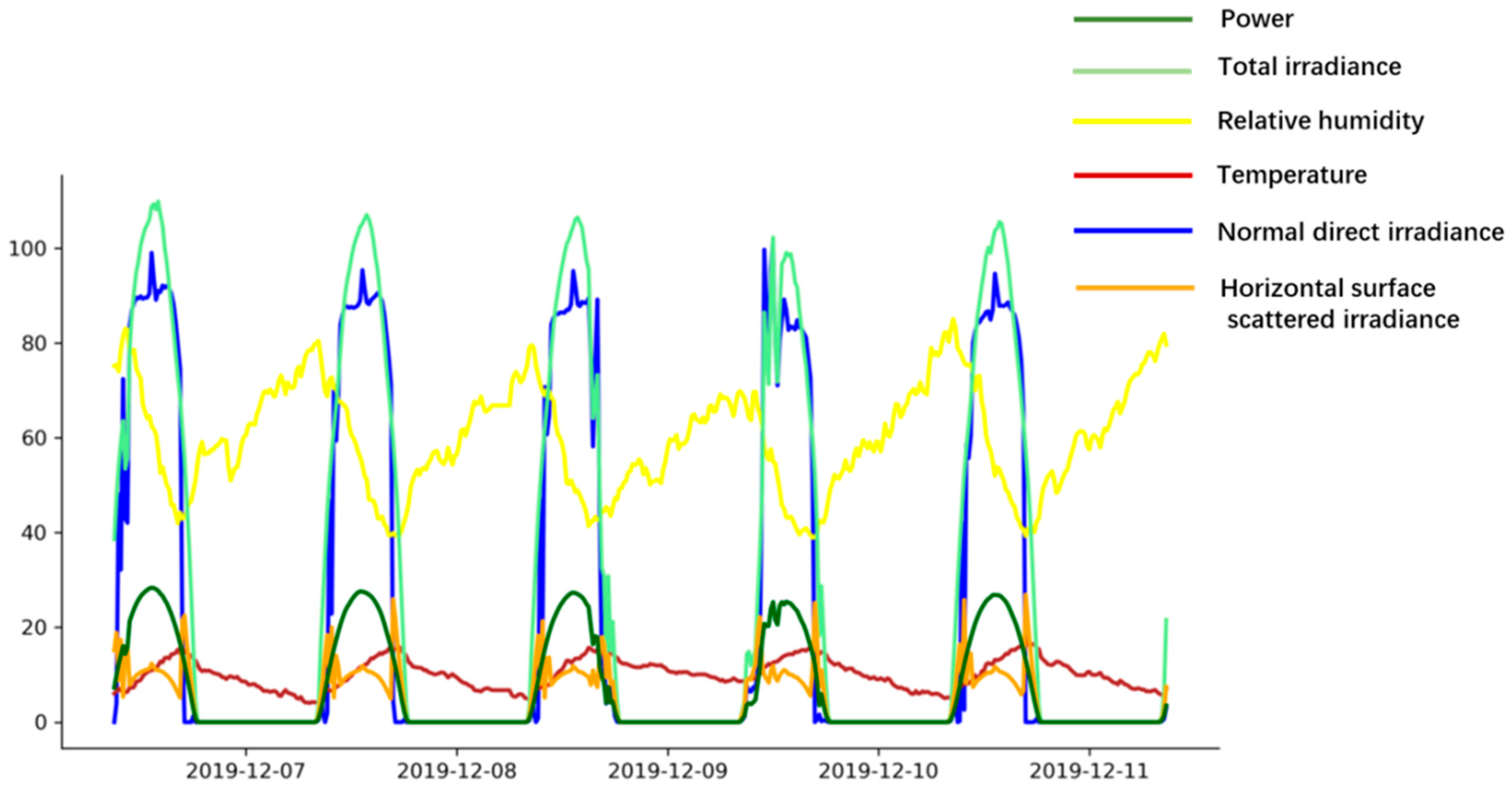
For deep learning models, more features as input are not better. Too many features may lead to data redundancy, which can affect the forecasting performance of the model. Therefore, this study explores the input feature combinations through experimental trial-and-error methods [27] and finally chooses daytime data of six features—total irradiance, normal direct irradiance, horizontal scattered irradiance, humidity, and temperature—as the final input feature data. Detailed statistics of the data from the three PV plants are shown in Table 1. As an example, Figure 4 shows the trends of these variables with respect to power for five consecutive days (all irradiance values are scaled down by a factor of 10 for clarity and intuition) on dataset 1, from which a clear correlation can be seen between the trends of these weather variables with respect to power.
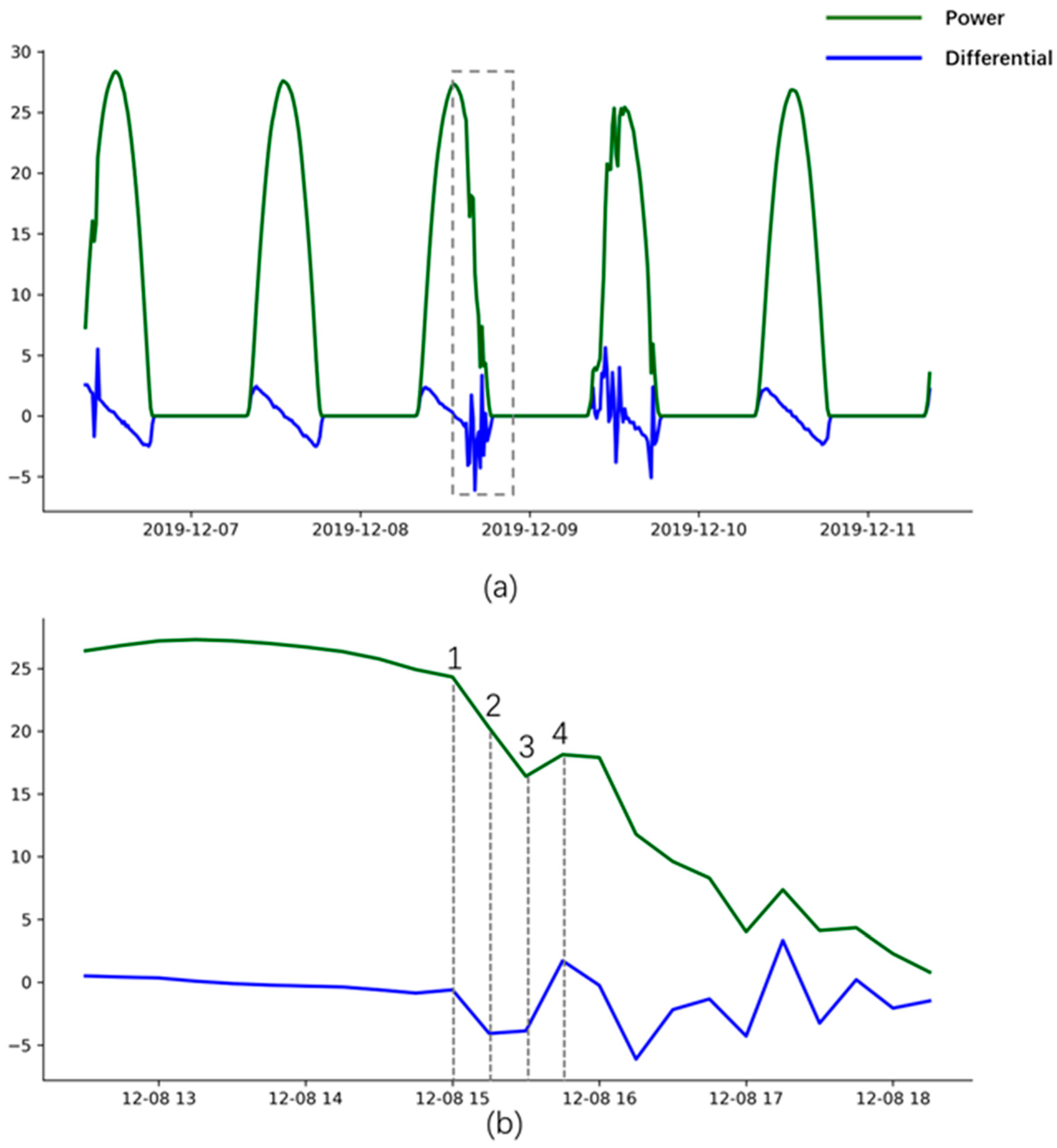
In addition, this study innovatively introduces the first-order difference series of the power as a special auxiliary feature variable of the model (already detailed in Section 2.3). The first-order difference series is the difference between every two neighboring observations in the original time series. For the time series y t , its first-order difference series Δ y t is defined as
Δ y t = y t y t 1
where y t is the observation at time t , and y t - 1 is the observation at time t - 1 . By calculating the difference between neighboring time points, the first-order difference series can reveal short-term fluctuation trends and local changes in the time series. If the values of the first-order difference show significant changes in different time periods, this usually means that there is a fluctuation trend in the original time series. Such fluctuating trends can help us better understand whether there are upward or downward trends in the time series and the magnitude of changes in these trends. Therefore, using the first-order difference series as an input feature to the forecasting model can inject more a priori knowledge about PV power fluctuations into the model. As an example, for dataset 1, Figure 5a gives a trend comparison plot of the PV power series with its first-order difference series for five consecutive days, and Figure 5b is a zoom-in of the dashed box part of Figure 5a for the interval from 12:00 noon to 18:00 p.m. on 8 December. In the figure, it can be seen that the PV power differential sequence contains the dynamic change (fluctuation) features of the power in the adjacent moments before and after. For example, the power basically has no fluctuation before the corresponding moment (15:00) of point 1, and the differential curve is flat. Starting from point 1, the power starts to decrease rapidly, and the difference series shows a downward trend, indicating that the power starts to fluctuate. Although the power decreases from point 1 to point 3, the difference series shows that this fluctuation trend is only maintained until point 2, and the PV power does not fluctuate again from point 2 but maintains this downward trend until point 3, and then the PV power starts to rise from point 3, corresponding to an upward trend in the difference series, which indicates that the power fluctuates upward once again. In conclusion the difference series can reflect the fluctuation trend of PV power in adjacent moments, which helps the model to learn the power ramp.
In summary, we use the historical PV power first-order difference series as the input to the model along with several other weather variables and group the features according to the different mechanisms of network feature extraction (already detailed in Section 2.3). The entire dataset is divided into two major parts: 90% for the training set (of which 20% is used for the validation set) and 10% for the test set [28].

4.2. Experimental Task Setup

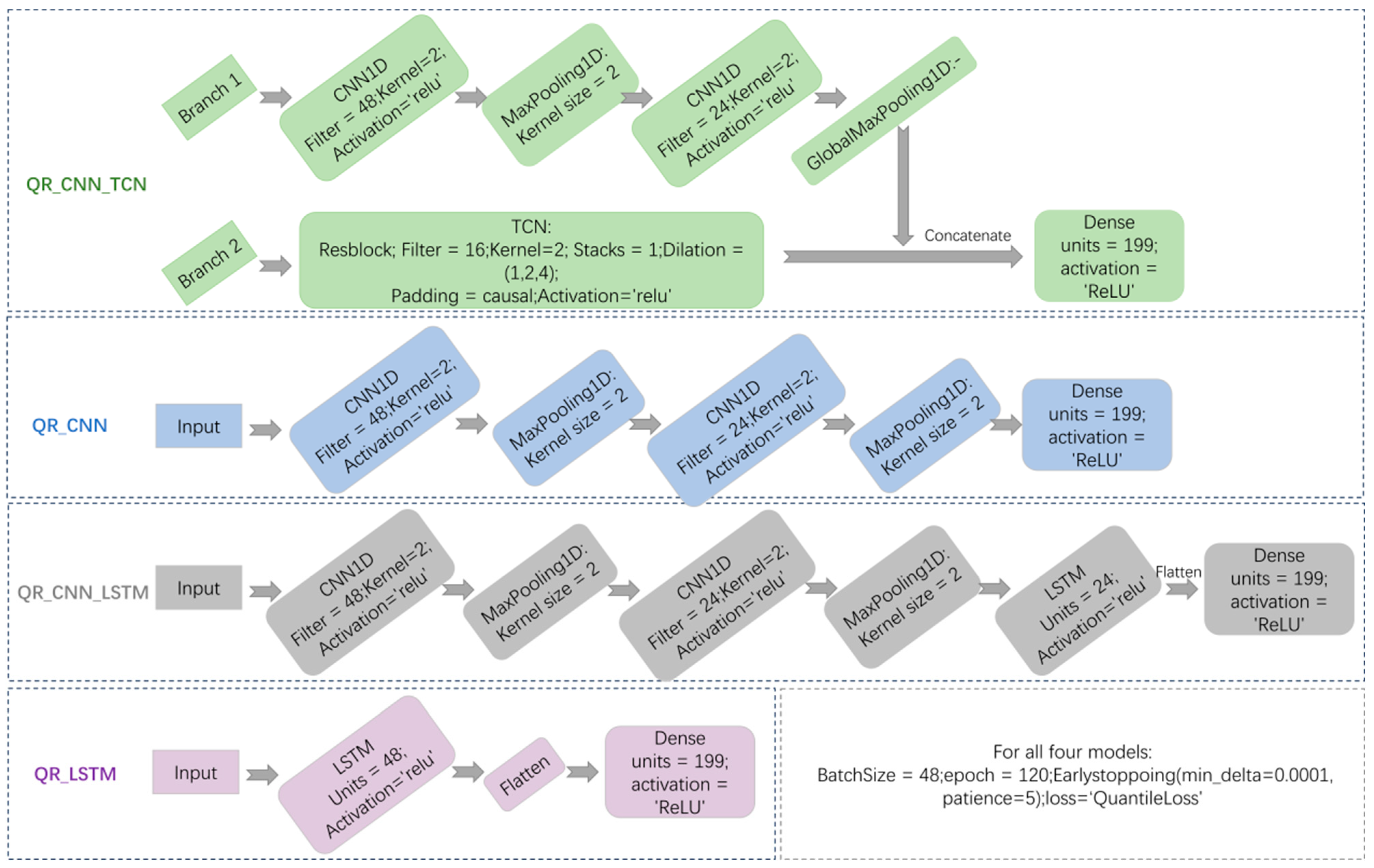
In this paper, three sets of experimental tasks are executed: (1) Point-forecasting experiments. (2) Interval-forecasting experiments. (3) Probabilistic-forecasting experiments. In order to validate the comprehensive performance of the proposed models, we select LSTM, CNN, and CNN_LSTM [34] combined with QR, which are deep learning models with excellent forecasting performance in the domain, as the benchmark comparison models. The framework and parameter settings of the models involved in this paper are shown in Figure 6. All parameters are set by trial and error [28].

4.2.1. Point-Forecasting Tasks

For the point-forecasting task, three experiments are carried out in this study:
(1) To verify the performance of the proposed model dual-input, dual-branch architecture, branch ablation experiments are conducted. The experimental results are shown in Table 2, where “Input 1_QRCNN” represents the QRCNN branching model with historical power sequences and their difference sequences as inputs, and “Input 2_QRTCN” represents the QRTCN branching model with several other meteorological feature sequences and historical power sequences as input to the QRTCN branching model.
It can be seen that the forecasting accuracy of both models with a single-input, single-branch structure is lower than that of the model with a double-input, double-branch structure on three different datasets, and this indicates that the model architecture design method in this paper, which is based on the operation mechanism of the model and combines the a priori knowledge to match the input feature data, can capture more time-scale feature information and improve the forecasting performance of the model.
(2) To verify the superiority of this study in incorporating a priori knowledge of the target sequence at the input level, ablation experiments of differential feature sequences are conducted. The experimental results are shown in Table 3, where “QR_CNN_TCN (no_diff)” represents the model without differential sequence feature input.
In the experimental results, it can be seen that the model that adds the PV power difference sequence as a new auxiliary feature to the input obtains better forecasting accuracy on all three datasets. This indicates that the introduction of the PV power difference sequence injects more a priori knowledge about the power variation trend into the model.
(3) In order to verify the comprehensive performance and applicability of the proposed models for point forecasting, baseline model comparison experiments were conducted on three different datasets. The forecasting results of all models on three different datasets are given in Table 4. Compared to other commonly used and state-of-the-art DL models in the field, the proposed method in this study exhibits better point-forecasting results on all three datasets. This also indicates that the proposed models have better applicability. On dataset 1, the proposed model shows more advantages, with a 9.8% boost in MAE and a 1% boost in RMSE compared to the best-performing QR_CNN_LSTM model among the other models. On dataset 2, the MAE boosts 5.3% and RMSE boosts 2% compared to the best-performing QR_CNN_LSTM model among the other models. On dataset 3, the MAE boosts 6.1% and RMSE boosts 3.2% compared to the best-performing QR_CNN model among the other models. In addition, all models obtained high R 2 on the three different datasets, indicating that all models are able to capture most of the patterns and relationships in the data. Compared to the other two datasets, on dataset 1, all models exhibit the optimal R 2 , 0.97.
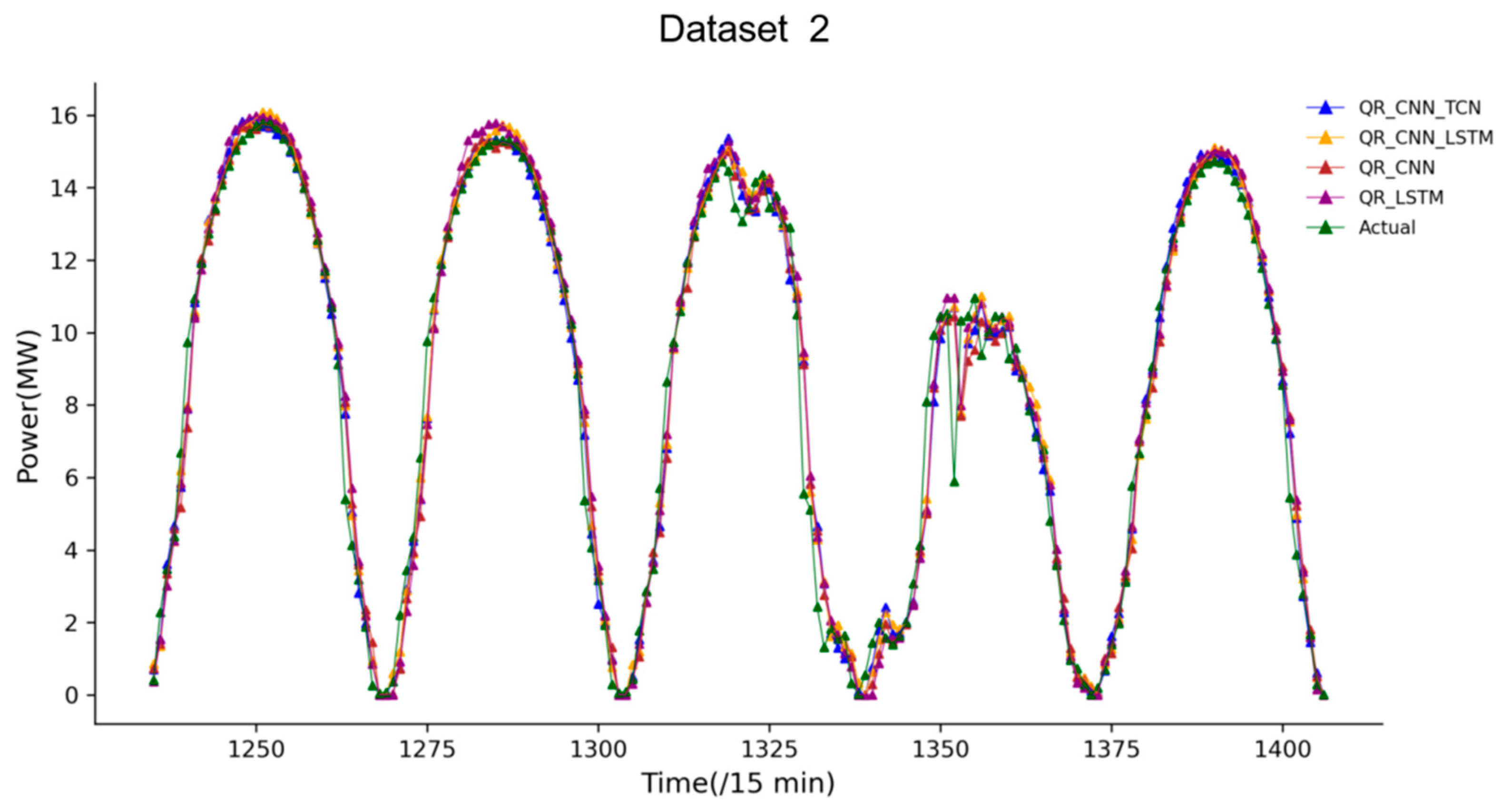
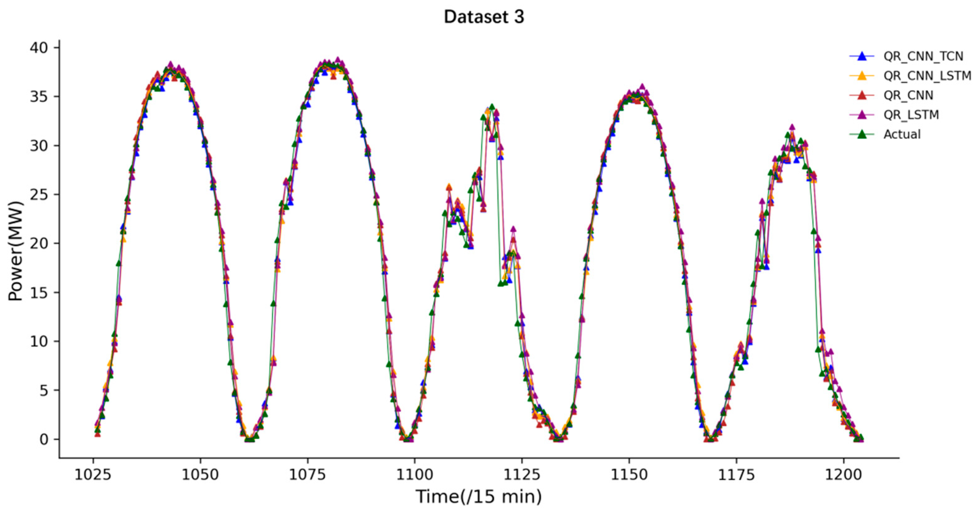
Figure 7, Figure 8 and Figure 9 visualize the line plots of point forecasting for all models for five consecutive days on three different datasets. It can also be seen that all models have a high ability to fit the real power. And the curve-fitting ability of the proposed model is the best among all models.

4.2.2. Interval-Forecasting Tasks

PV power interval forecasting can provide plant and system decision makers with a possible range of potential outcomes, which helps them to assess risk and develop strategies based on possible best- and worst-case scenarios. In order to validate the performance and applicability of the model interval forecasting, this study evaluates the forecasting results of all the models with 95% confidence intervals on three different datasets. Table 5 demonstrates the interval-forecasting results for all models. It can be seen that on all three datasets, the proposed model obtains the highest PICP and the lowest WS when compared with the baseline model, which indicates that the proposed model covers more observations while obtaining a narrower width of confidence intervals, has optimal interval-forecasting performance, and has good applicability. Taking dataset 1 as an example, the proposed model has the highest PICP of 96.9% and the smallest WS of 7.9. The QR_CNN_LSTM model, although having almost the same PICP (96.6%) as the proposed model, has a WS of 18.8. This indicates that, covering almost the same number of observations, the width of the confidence interval of the QR_CNN_LSTM model is almost 2.3 times that of the proposed model. Obviously, such a prediction interval introduces more uncertainty, which is unfavorable for the decision maker to make a correct decision. In comparison, the QR_CNN model performs relatively well, with a PICP slightly lower than the proposed model (at 95.5%) and a WS of 8.3.
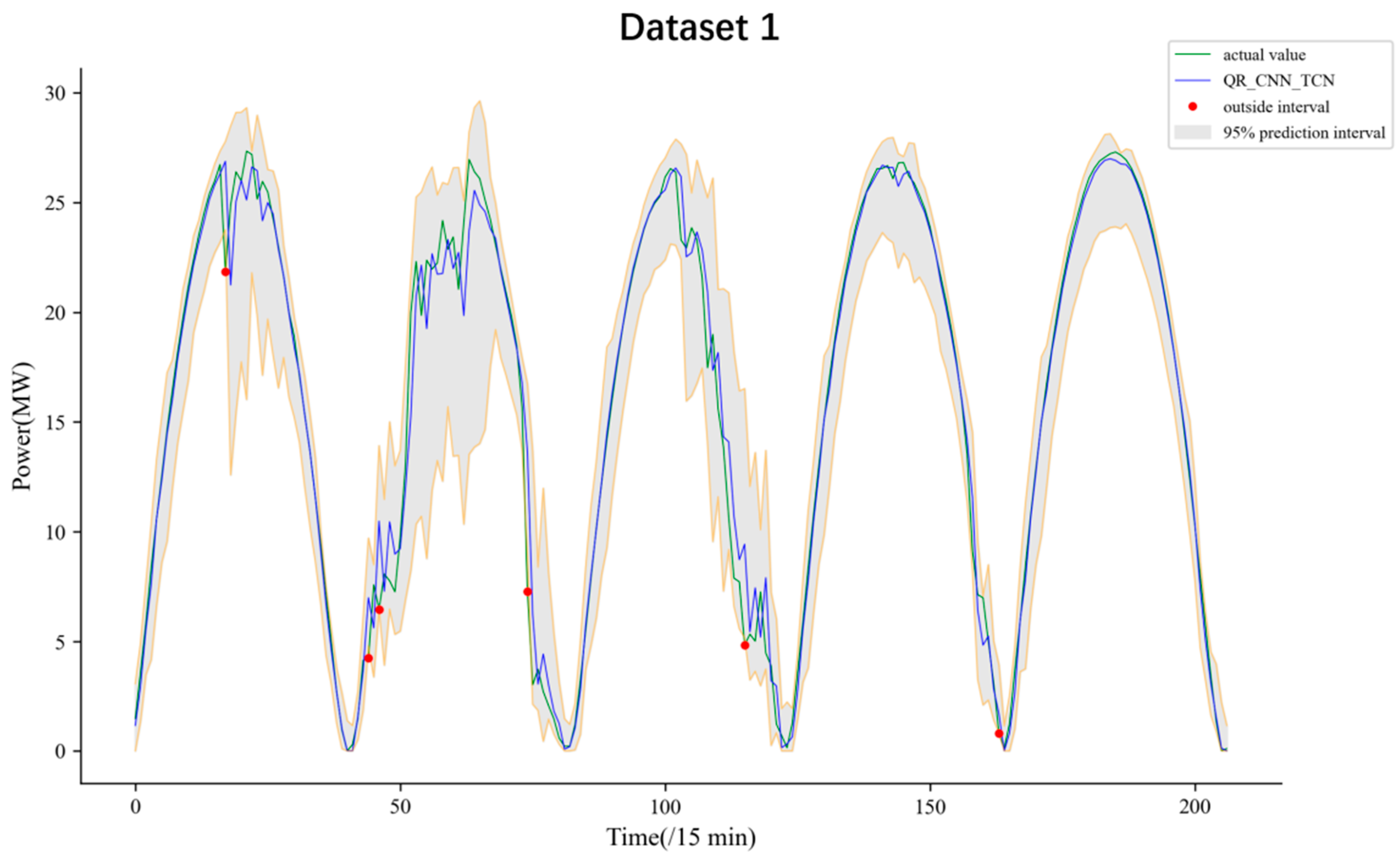
The interval-forecasting results presented in Table 5 are not intuitive, although they already demonstrate, in the form of evaluation metrics, that the proposed model optimizes the quality of uncertainty quantification on the interval-forecasting task, i.e., it covers more observations while obtaining a narrower width of confidence intervals. To give a more intuitive picture of how well the proposed model quantifies uncertainty, Figure 10, Figure 11 and Figure 12 plot the line graphs of the 95% confidence interval forecasts for five consecutive days on the three datasets. It can be seen that the prediction intervals of the model are wider where the fluctuations are large and narrower where the fluctuations are small. During the midday hours, although the radiation intensity is high, the solar radiation may fluctuate widely due to atmospheric conditions, cloud cover changes, and other factors, thus introducing large uncertainties. In addition, the temperature is usually higher during the midday hours, and due to the temperature effect, the output power of the PV module decreases as the temperature rises, thus introducing further uncertainty. All these lead to an increase in the uncertainty of the PV power, which makes the 95% confidence interval for the noon hour wider. Therefore, this forecast result is in accordance with the PV power output characteristics.
In addition, it can be seen in Figure 10, Figure 11 and Figure 12 that the lower boundaries of the prediction intervals are farther away from the actual observations compared to the upper boundaries, indicating that the model has relatively large uncertainty in forecasting the lower quantiles.
Meanwhile, in order to illustrate the impact of the proposed first-order difference feature of PV power as an auxiliary feature of the model on the interval-forecasting results, Table 6 demonstrates the interval-forecasting results with and without difference inputs under the proposed model architecture. It can be seen that the models with power first-order difference series as auxiliary features have better overall performance than the non-differential models on all three datasets, with higher PICP while having smaller WS.

4.2.3. Probabilistic-Forecasting Tasks

The purpose of the PV power probabilistic-forecasting task is to better predict the uncertainty of the PV output, and the assessment of the probabilistic-forecasting results synthesizes the deviation and uncertainty between the probability distribution of the models’ forecasting results and the actual observations. The evaluation of the probabilistic-forecasting results for each model on the three PV plant datasets is shown in Table 7. It can be seen that the model proposed in this paper obtains the lowest CRPS values on all three different PV plant datasets compared to other models. In dataset 1, the CRPS of the proposed model is 0.628, which has the smallest value. The QR_CNN_LSTM’s is 0.633, which has a slightly higher value than the proposed model and is very close to the probabilistic-forecasting performance of the proposed model. The QR_LSTM model has the worst performance of 0.847. The CRPS of the proposed model is improved by 25.8% compared to it. In dataset 2, the CRPS of the proposed model is improved by 3.4% compared to the best-performing QR_CNN model and 51.3% compared to the worst-performing QR_LSTM model. In dataset 3, the CRPS of the proposed model is very close to that of the best-performing QR_CNN model, which are 1.208 and 1.218, respectively. Compared with the worst-performing QR_LSTM model, the CRPS is improved by 10%. Such probabilistic-forecasting results show that the distribution predicted by the proposed model is much closer to the true distribution of the observations, with the best forecasting accuracy and reliability and the most comprehensive performance. Figure 13 gives a comparison of the three forecasting results of each model on the three datasets. It can be seen that the probabilistic-forecasting results of the proposed model are consistent with the corresponding point-forecasting results and interval-forecasting results, indicating that for the proposed model, good point-forecasting results produce good interval and probabilistic-forecasting results, and the model is superior in all aspects.
In this study, we post-process the discrete quantile forecast results using a KDE method incorporating 5-fold cross-validation in order to obtain a more continuous and smooth probability density distribution. This helps power system decision makers to use continuous probabilistic information in their decisions, which is important for downstream applications such as energy management and scheduling. As an example, Figure 14 shows the probability density curves of the proposed model on dataset 1 at 9 sampling points (sampling the test set in 8 equal parts). As can be seen in the results, the overall shapes of these curves are basically similar, with relatively full contours. And their widths and heights are also moderate, indicating that the probability density curves obtained using the KDE method combined with cross-validation are valid. At time periods 828, 1034, 1448, and 1655 in the test set, the observation point is located at the center of the probability density curve. The observations are very close to the center of the probability density curve at time periods 1, 414, and 621. This indicates that the model’s forecasting accuracy is very high for all of these time periods. At time periods 207 and 1241, the observations are off the center of the probability density curve. This indicates that the model’s forecast error is high in these time periods. Overall, the forecast results are reliable for most of the time periods and can be used to assist power system decision makers in making decisions. In addition, there is a degree of long tailing around the 0 value on the left side of each of these curves, indicating that the model is relatively conservative in its forecasts for the lower quantiles. This is consistent with the interval-forecasting results.
In summary, by calculating the CRPS of the forecast results, it can be seen that the match between the forecast probability distributions of the proposed model and the actual observations is the best among all the models on the three different plant data, which indicates that the consistency between the forecasts and the actual observations is better, and the forecasts are more accurate, with optimal comprehensive performance. It also shows that the model has better suitability on different data. In addition, the probability density curves of the forecast results obtained by the KDE method combined with cross-validation are full of contours with moderate width and height, which form an effective probability density function estimation. The sampling curves show that the forecasting results of the proposed model are reliable in most of the time periods, which can provide decision support for power system decision makers.

5. Conclusions and Discussion

PV power forecasting and its potential uncertainty have an important impact on the safe and stable operation of the power system and rational decision making in the energy market. The introduction of domain a priori knowledge can enhance the model’s expressive ability by more accurately representing the data features and fully utilizing the computational advantages of the DL model. In view of this, this study is based on the deep integration of the feature extraction mechanism of DL algorithms with PV power data and gives full play to the high-dimensional nonlinear processing capability of DL models and the advantages of nonparametric QR methods to adapt to various complex and nonstandard data forms, and proposes a deep learning QR method with a priori knowledge injection to perform the task of ultra-short-term PV power probabilistic forecasting. The method deeply integrates the algorithm with the data under the premise of injecting more a priori knowledge from the perspectives of input feature engineering and model architecture design: in the aspect of model input feature engineering, this study innovatively introduces the first-order difference sequences of the target series into the input of the DL model as the a priori features, which injects more short-term and local fluctuation information about the PV power into the model and classifies them into two groups together with other meteorological features to provide different constraints on feature sequences for the two branch models; in terms of model architecture design, this study innovatively matches the different computing mechanisms of CNN and TCN with the two groups of input features to form two branches of the network that learn different feature relationships. This method realizes the dual integration of a priori knowledge in the model feature input layer and the model architecture and combines the QR method with the two-branch DL model for multi-task learning to realize the multi-quantile forecasting of PV power. Finally, a reliable probability density distribution of the PV power series is obtained by KDE combined with cross-validation methods.
The experimental results show the following:
(1)
The first-order difference series of the target sequence as the input to the model can provide the model with more trend information of the target sequence on the ultra-short-term time scale, which improves the forecasting performance of the model and the comprehensibility of the model output.
(2)
The model architecture design that selectively integrates the DL model operation mechanism with the input data containing different information can realize the extraction of targeted information so that the model can learn finer feature information, which improves the forecasting performance of the model and the comprehensibility of the model output.
(3)
Combining QR with two branches of DL models, CNN and TCN, enables the proposed method to simultaneously perform multi-task learning and knowledge fusion in both branch models, which, in combination with the KDE method, obtains high-quality interval-forecasting results and probabilistic-forecasting results. In addition, in the interval-forecasting results (Figure 10, Figure 11 and Figure 12), it is found that the upper boundary of the forecasting intervals is closer than the true values, while the lower boundary is farther away, indicating that the model is relatively conservative in predicting the lower quantiles, which is consistent with the results exhibited by the probability density curves (Figure 14). In subsequent studies, the model will be further optimized from two perspectives, namely, input data sparsity and model nonlinear processing capability, to reduce the uncertainty at low power values.
(4)
Compared to the state-of-the-art deep learning models in the field combined with QR, the model proposed in this study shows the most superior performance on three different datasets, either point forecasting, interval forecasting, or probabilistic forecasting. This also indicates the good applicability of the proposed model to new data. The proposed method can provide technical support to the decision makers of PV farms and power systems in assessing risks and formulating strategies.
In conclusion, with the improvement in computing power and the development of big data technology, nonparametric probabilistic-forecasting methods based on DL are gradually attracting attention from both academia and industry. They are able to adapt to more complex data structures and patterns without relying on data distribution assumptions, providing greater flexibility and adaptability. The proposed method in this study can provide new ideas for the forecasting task of data with complex patterns such as PV power and wind power.

Author Contributions

Conceptualization, X.R., F.Z. and Y.L.; Data curation, X.R. and L.L.; Funding acquisition, X.R.; Methodology, X.R., Y.L. and F.Z.; Software, X.R.; Visualization, L.L. and F.Z.; Writing—original draft, X.R. All authors have read and agreed to the published version of the manuscript.

Funding

This research work was supported by the Inner Mongolia Natural Science Foundation, No. 2024MS06018, and the Inner Mongolia Autonomous Region Key R&D and Achievement Transformation Program Project, No. 2022YFSJ0033.

Data Availability Statement

PV plant operators require data to be kept confidential.

Conflicts of Interest

Author Lingfeng Li was employed by the company Inner Mongolia Huadian New Energy Co. The remaining authors declare that the research was conducted in the absence of any commercial or financial relationships that could be construed as a potential conflict of interest.

References

  1. IEA. Renewable Capacity Growth by Technology, Main and Accelerated Cases, 2005–2028; IEA: Paris, France, 2023; Available online: https://www.iea.org/data-and-statistics/charts/renewable-capacity-growth-by-technology-main-and-accelerated-cases-2005-2028 (accessed on 3 March 2024.).
  2. Liu, Y.; Ye, L.; Qin, H.; Hong, X.; Ye, J.; Yin, X. Monthly streamflow forecasting based on hidden Markov model and Gaussian Mixture Regression. J. Hydrol. 2018, 561, 146–159. [Google Scholar] [CrossRef]
  3. Li, Y.; He, S.; Li, Y.; Ge, L.; Lou, S.; Zeng, Z. Probabilistic charging power forecast of EVCS: Reinforcement learning assisted deep learning approach. IEEE Trans. Intell. Veh. 2022, 8, 344–357. [Google Scholar] [CrossRef]
  4. Wang, J.; Tang, X.; Jiang, W. A deterministic and probabilistic hybrid model for wind power forecasting based improved feature screening and optimal Gaussian mixed kernel function. Expert Syst. Appl. 2024, 251, 123965. [Google Scholar] [CrossRef]
  5. Heng, J.; Hong, Y.; Hu, J.; Wan, S. Probabilistic and deterministic wind speed forecasting based on non-parametric approaches and wind characteristics information. Appl. Energy 2022, 306 Pt A, 118029. [Google Scholar] [CrossRef]
  6. Lin, Y.; Yang, M.; Wan, C.; Wang, J.; Song, Y. A multi-model combination approach for probabilistic wind power forecasting. IEEE Trans. Sustain. Energy 2019, 10, 226–237. [Google Scholar] [CrossRef]
  7. Qi, S.; Peng, H.; Zhang, X.; Tan, X. Is energy efficiency of Belt and Road Initiative countries catching up or falling behind? Evidence from a panel quantile regression approach. Appl. Energy 2019, 253, 113581. [Google Scholar] [CrossRef]
  8. Bracale, A.; Carpinelli, G.; De Falco, P. A probabilistic competitive ensemble method for short-term photovoltaic power forecasting. IEEE Trans. Sustain. Energy 2016, 8, 551–560. [Google Scholar] [CrossRef]
  9. Ma, X.; Du, H.; Wang, K.; Jia, R.; Wang, S. An efficient QR-BiMGM model for probabilistic PV power forecasting. Energy Rep. 2022, 8, 12534–12551. [Google Scholar] [CrossRef]
  10. Wang, G.B.; Wang, H.Z.; Li, G.Q.; Peng, J.C.; Liu, Y.T. Deep belief network based point and probabilistic wind speed forecasting approach. Appl. Energy 2016, 182, 80–93. [Google Scholar] [CrossRef]
  11. Ye, Y.; Shao, Y.; Li, C.; Hua, X.; Guo, Y. Online support vector quantile regression for the dynamic time series with heavy-tailed noise. Appl. Soft Comput. 2021, 110, 107560. [Google Scholar] [CrossRef]
  12. Yang, D.; Gueymard, C.A. Probabilistic post-processing of gridded atmospheric variables and its application to site adaptation of shortwave solar radiation. Sol. Energy 2021, 225, 427–443. [Google Scholar] [CrossRef]
  13. Mayer, M.J.; Yang, D. Probabilistic photovoltaic power forecasting using a calibrated ensemble of model chains. Renew. Sustain. Energy Rev. 2022, 168, 112821. [Google Scholar] [CrossRef]
  14. de Barros Silva, A.W.; Freitas, B.B.; de Alencar Filho, C.L.; de Freitas, C.D.; de Sousa Junior, E.A.; de Castro, E.S.; de Araújo, E.M.; Correia, F.I.F.; da Silva, F.R.P.; de Souza, J.J.S.; et al. Methodology based on artificial neural networks for hourly forecasting of PV plants generation. IEEE Latin Am. Trans. 2022, 20, 659–668. [Google Scholar] [CrossRef]
  15. Zuo, H.M.; Qiu, J.; Jia, Y.H.; Wang, Q.; Li, F.F. Ten-minute prediction of solar irradiance based on cloud detection and a long short-term memory (LSTM) model. Energy Rep. 2022, 8, 5146–5157. [Google Scholar] [CrossRef]
  16. Chandel, S.S.; Gupta, A.; Chandel, R.; Tajjour, S. A Review of deep learning techniques for power generation prediction of industrial solar photovoltaic plants. Sol. Compass 2023, 8, 100061. [Google Scholar] [CrossRef]
  17. Wang, Z.; Wang, C.; Cheng, L.; Li, G. An approach for day-ahead interval forecasting of photovoltaic power: A novel DCGAN and LSTM based quantile regression modeling method. Energy Rep. 2022, 8, 14020–14033. [Google Scholar] [CrossRef]
  18. Li, Y.; Zhang, M.; Chen, C. A deep-learning intelligent system incorporating data augmentation for short-term voltage stability assessment of power systems. Appl. Energy 2022, 308, 118347. [Google Scholar] [CrossRef]
  19. Liu, R.; Wei, J.; Sun, G.; Muyeen, S.M.; Lin, S.; Li, F. A short-term probabilistic photovoltaic power prediction method based on feature selection and improved LSTM neural network. Electr. Power Syst. Res. 2022, 210, 108069. [Google Scholar] [CrossRef]
  20. Wang, H.; Yi, H.; Peng, J.; Wang, G.; Liu, Y.; Jiang, H.; Liu, W. Deterministic and probabilistic forecasting of photovoltaic power based on deep convolutional neural network. Energy Convers. Manag. 2017, 153, 409–422. [Google Scholar] [CrossRef]
  21. Jiang, H.; Dong, Y. A nonlinear support vector machine model with hard penalty function based on glowworm swarm optimization for forecasting daily global solar radiation. Energy Convers Manag. 2016, 126, 991–1002. [Google Scholar] [CrossRef]
  22. Huang, Q.; Wei, S. Improved quantile convolutional neural network with two-stage training for daily-ahead probabilistic forecasting of photovoltaic power. Energy Convers. Manag. 2020, 220, 113085. [Google Scholar] [CrossRef]
  23. Du, H.; Ma, X.; Jia, R. A Novel Deep Learning Fusion Model for Probabilistic Prediction of Photovoltaic Power. In Proceedings of the 2022 4th International Conference on Power and Energy Technology (ICPET), Beijing, China, 28–31 July 2022; pp. 774–781. [Google Scholar] [CrossRef]
  24. Bai, S.; Kolter, J.Z.; Koltun, V. An Empirical Evaluation of Generic Convolutional and Recurrent Networks for Sequence Modeling. arXiv 2018, arXiv:1803.01271. [Google Scholar] [CrossRef]
  25. Limouni, T.; Yaagoubi, R.; Bouziane, K.; Guissi, K.; Baali, E.H. Accurate one step and multistep forecasting of very short-term PV power using LSTM-TCN model. Renew. Energy 2023, 205, 1010–1024. [Google Scholar] [CrossRef]
  26. Fu, H.; Zhang, J.; Xie, S. A Novel Improved Variational Mode Decomposition-Temporal Convolutional Network-Gated Recurrent Unit with Multi-Head Attention Mechanism for Enhanced Photovoltaic Power Forecasting. Electronics 2024, 13, 1837. [Google Scholar] [CrossRef]
  27. Ren, X.; Zhang, F.; Sun, Y.; Liu, Y. A Novel Dual-Channel Temporal Convolutional Network for Photovoltaic Power Forecasting. Energies 2024, 17, 698. [Google Scholar] [CrossRef]
  28. Ren, X.; Zhang, F.; Zhu, H.; Liu, Y. Quad-kernel deep convolutional neural network for intra-hour photovoltaic power forecasting. Appl. Energy 2022, 323, 119682. [Google Scholar] [CrossRef]
  29. Glendinning, R.H.; Scott, D.W. Multivariate Density Estimation, Theory, Practice and Visualization; Journal of the Royal Statistical Society Series D: The Statistician 1; John Wiley & Sons: Hoboken, NJ, USA, 2018; Volume 1. [Google Scholar] [CrossRef]
  30. Wahbah, M.; Mohandes, B.; EL-Fouly, T.H.; El Moursi, M.S. Unbiased cross-validation kernel density estimation for wind and PV probabilistic modelling. Energy Convers. Manag. 2022, 266, 115811. [Google Scholar] [CrossRef]
  31. Xu, C.; Sun, Y.; Du, A.; Gao, D.-C. Quantile regression based probabilistic forecasting of renewable energy generation and building electrical load: A state-of-the art review. J. Build. Eng. 2023, 79, 107772. [Google Scholar] [CrossRef]
  32. Lauret, P.; David, M.; Pedro, H.T.C. Probabilistic solar forecasting using quantile regression models. Energies 2017, 10, 1591. [Google Scholar] [CrossRef]
  33. Pinson, P.; Reikard, G.; Bidlot, J.-R. Probabilistic forecasting of the wave energy flux. Appl. Energy 2012, 93, 364–370. [Google Scholar] [CrossRef]
  34. Wang, K.; Qi, X.; Liu, H. A comparison of day-ahead photovoltaic power forecasting models based on deep learning neural network. Appl. Energy 2019, 251, 113315. [Google Scholar] [CrossRef]
Figure 1. The overall research flowchart of the proposed method.
Energies 17 04026 g001
Figure 2. Structure of the TCN model.
Energies 17 04026 g002
Figure 3. A schematic of the structure of the proposed model.
Energies 17 04026 g003
Figure 4. Trends in input feature variables for five consecutive days in dataset 1.
Energies 17 04026 g004
Figure 5. Trend comparison of the PV power series with its first-order difference series. (a) PV power series for five consecutive days with its first-order difference series. (b) Enlarged view of the dotted box in (a).
Energies 17 04026 g005
Figure 6. Parameter settings and data flow for each model.
Energies 17 04026 g006
Figure 7. The line graph of point predictions for all models on dataset 1 for 5 consecutive days.
Energies 17 04026 g007
Figure 8. The line graph of point predictions for all models on dataset 2 for 5 consecutive days.
Energies 17 04026 g008
Figure 9. The line graph of point predictions for all models on dataset 3 for 5 consecutive days.
Energies 17 04026 g009
Figure 10. Results of 5 consecutive days of day interval forecasting for the proposed model on dataset 1.
Energies 17 04026 g010
Figure 11. Results of 5 consecutive days of day interval forecasting for the proposed model on dataset 2.
Energies 17 04026 g011
Figure 12. Results of 5 consecutive days of day interval forecasting for the proposed model on dataset 3.
Energies 17 04026 g012
Figure 13. Comparison of the three forecasting results of each model on the three datasets.
Energies 17 04026 g013
Figure 14. Probability density curves for the proposed model on dataset 1 at 9 sampling points.
Energies 17 04026 g014
Table 1. Detailed statistics of the data from the three PV plants.
DatasetsStatistical ItemsFeatures
Power (MW)TI (w/m2)HI (w/m2)NI (w/m2)RH (%)Tem (°C)
Dataset 1 (35 MW, 17,255 samples)Mean13.4512.8110.9457.949.122.7
Std9.2365.559.7367.324.25.7
Min. value0.010002.54.0
Max. value30.871287.6289.21179.897.936.7
Dataset 2 (20 MW, 16,498 samples)Mean7.4437.845.8245.258.511.2
Std5.8328.936.9196.221.613.6
Min. value0.010004.38−26.5
Max. value19.471125.2148.8792.010038.2
Dataset 3 (50 MW, 17,346 samples)Mean19.6522.4149.8127.417.617.6
Std13.7357.9140.4209.216.413.6
Min. value0.010000−16.7
Max. value48.31328.0989.0923.069.741.2
The abbreviations “Std”, “TI”, “HI”, “NI”, “Tem”, and “RH” in the table stand for “Standard deviation”, “Total irradiance”, “Horizontal surface scattered irradiance”, “Normal direct irradiance”, “Temperature”, and “Relative humidity”, respectively.
Table 2. Comparison of the forecasting results of the proposed model and the two single-branch input models.
ModelDataset 1 (35 MW)Dataset 2 (20 MW)Dataset 3 (50 MW)
MAERMSEMAERMSEMAERMSE
QR_CNN_TCN0.7851.5620.6221.1341.5502.612
Input 1_QRCNN0.9041.6030.7941.3321.7542.787
Input 2_QRTCN0.8701.5960.7011.2011.7422.776
Bolded text in the table indicates optimal results.
Table 3. Comparison of the forecasting results of the proposed model and the model without differential features.
ModelDataset 1 (35 MW)Dataset 2 (20 MW)Dataset 3 (50 MW)
MAERMSEMAERMSEMAERMSE
QR_CNN_TCN0.7851.5620.6221.1341.5502.612
QR_CNN_TCN (non_diff)0.8271.5640.6891.1971.6382.702
Bolded text in the table indicates optimal results.
Table 4. Comparison of point-forecasting results of the proposed model with those of the baseline model.
ModelDataset 1 (35 MW)Dataset 2 (20 MW)Dataset 3 (50 MW)
MAERMSER2MAERMSER2MAERMSER2
QR_CNN_TCN0.7851.5620.970.6221.1340.961.5502.6120.96
QR_CNN_LSTM0.8701.5770.970.6571.1570.961.6822.7190.96
QR_LSTM1.0721.7160.970.7011.2130.961.7752.7960.96
QR_CNN0.9331.6140.970.6771.1960.961.6512.6980.96
Bolded text in the table indicates optimal results.
Table 5. Interval prediction results for all models on the three datasets.
ModelDataset 1 (35 MW)Dataset 2 (20 MW)Dataset 3 (50 MW)
PICP (%)WSPICP (%)WSPICP (%)WS
QR_CNN_TCN96.97.994.15.394.414.3
QR_CNN_LSTM [29]96.618.891.85.9292.617.3
QR_LSTM93.219.592.76.2991.829.3
QR_CNN95.58.391.46.4290.616.4
Bolded text in the table indicates optimal results.
Table 6. Comparison of interval prediction results with and without differential inputs for the proposed model architecture.
ModelDataset 1 (35 MW)Dataset 2 (20 MW)Dataset 3 (50 MW)
PICP (%)WSPICP (%)WSPICP (%)WS
QR_CNN_TCN96.97.994.15.394.414.3
QR_CNN_TCN (non_ diff)90.28.693.15.793.014.5
Bolded text in the table indicates optimal results.
Table 7. Probabilistic forecast evaluation index (CRPS) for all models.
ModelDataset 1 (35 MW)Dataset 2 (20 MW)Dataset 3 (50 MW)
QR_CNN_TCN0.6280.3041.208
QR_CNN_LSTM0.6330.4991.253
QR_LSTM0.8470.6241.329
QR_CNN0.7020.3381.218
Bolded text in the table indicates optimal results.
Disclaimer/Publisher’s Note: The statements, opinions and data contained in all publications are solely those of the individual author(s) and contributor(s) and not of MDPI and/or the editor(s). MDPI and/or the editor(s) disclaim responsibility for any injury to people or property resulting from any ideas, methods, instructions or products referred to in the content.