Article

Robust Energy Management Policies for Solar Microgrids via Reinforcement Learning

1
Department of Industrial and Systems Engineering, University of Tennessee, Knoxville, TN 37996, USA
2
School of Accounting, Southwestern University of Finance and Economics, Chengdu 610074, China
*
Author to whom correspondence should be addressed.
Energies 2024, 17(12), 2821; https://doi.org/10.3390/en17122821
Submission received: 23 April 2024 / Revised: 15 May 2024 / Accepted: 4 June 2024 / Published: 8 June 2024

Abstract

:
As the integration of renewable energy expands, effective energy system management becomes increasingly crucial. Distributed renewable generation microgrids offer green energy and resilience. Combining them with energy storage and a suitable energy management system (EMS) is essential due to the variability in renewable energy generation. Reinforcement learning (RL)-based EMSs have shown promising results in handling these complexities. However, concerns about policy robustness arise with the growing number of grid intermittent disruptions or disconnections from the main utility. This study investigates the resilience of RL-based EMSs to unforeseen grid disconnections when trained in grid-connected scenarios. Specifically, we evaluate the resilience of policies derived from advantage actor–critic (A2C) and proximal policy optimization (PPO) networks trained in both grid-connected and uncertain grid-connectivity scenarios. Stochastic models, incorporating solar energy and load uncertainties and utilizing real-world data, are employed in the simulation. Our findings indicate that grid-trained PPO and A2C excel in cost coverage, with PPO performing better. However, in isolated or uncertain connectivity scenarios, the demand coverage performance hierarchy shifts. The disruption-trained A2C model achieves the best demand coverage when islanded, whereas the grid-connected A2C network performs best in an uncertain grid connectivity scenario. This study enhances the understanding of the resilience of RL-based solutions using varied training methods and provides an analysis of the EMS policies generated.

1. Introduction

As our world moves toward increasing the use of renewable energy sources (RES), the inherent uncertainties in energy production necessitate energy storage systems (ESS) with optimal energy management strategies (EMS) [1]. This need for optimal EMSs is also known as the energy management problem (EMP), which is a broad term covering many outcomes of energy system dynamics [2]. Optimal EMSs will supply auxiliary power when RESs fall short, store excess energy when RESs generate more than needed, and adapt to the unpredictable nature of RES energy production [3]. The energy management agent that controls the ESS must be able to meet some set objectives by appropriately discharging, charging, or idling the ESS. Microgrids (MGs), or small localized energy grids, can increase resilience to unforeseen power disruptions in the utility grid by providing a local controllable power source. MGs can provide power to their designated load in conjunction with the main utility or in island mode, where they are the sole power source. Microgrids are often paired with renewable distributed generation (DGs) energy sources such as photovoltaic generation (PV) units, which have been shown to be capable of supplying electricity during unexpected grid outages [4]. Often, the goal of the stakeholders of the distributed generation microgrid (DGMG) is to maximize the cost and demand coverage of the facilities involved. However, with increasing extreme weather events [4,5] and system load [6], increases in unexpected disruptions can occur, causing large populations to go without power for extended periods. When working alongside the main grid, the DGMG can offset energy expenses by supplying power from local sources, eliminating the necessity to buy electricity. In areas where programs allow for the sale of excess energy back to the grid, profits can be attained through optimal EMS strategies. When isolated from the main grid, the cost of buying energy becomes irrelevant and the goal becomes maximizing load coverage with any energy sources available.
Achieving resilience in DGMGs against unforeseen disruptions requires optimal EMS for both grid-connected and islanded cases. Ensuring microgrids are resilient to unexpected events is essential for providing safe, reliable, and stable energy. The increasing integration of renewable energy sources (RES) introduces unique challenges that need optimal solutions to minimize disruptions. Robust EMS is crucial in any scenario. This study explores how EMS strategies derived from reinforcement learning (RL) with different training methods offer robust solutions. It compares the effectiveness of proximal policy optimization (PPO) and advantage actor–critic network (A2C) deep reinforcement learning (DRL) agents in achieving optimal EMS in grid-connected, islanded, and connection-uncertain cases. These RL algorithms learn through experience without needing a predefined model. The two methods are trained on grid-connected and grid-uncertain simulations of a microgrid, producing four networks. Simulations for grid-connected scenarios compare the cost and demand coverage of the trained networks, while the other scenarios focus on demand coverage only. The performance of the trained networks is compared to load-focused heuristic and random operation approaches as baselines.
To train the RL EMS agents, a simulation of an MG based on data for hourly building loads and photo-voltaic (PV) unit output in Knoxville, TN, is performed to train the agents and generate their EMS policies. Grid-connected scenarios aim to maximize the potential sell-back profits and cost covered by the DG unit based on local on- and off-peak energy prices. The average hourly cost covered for PPO- and A2C-trained networks and a demand coverage greedy algorithm is compared. Next, a simulation of the MG isolated from the main grid is performed to train and test the ability of RL agents to meet hourly energy demand in an isolated case where meeting demands and not cost becomes the objective. Efforts were made to train the RL agents in only isolated cases as well as scenarios where there are intermittent losses in grid connectivity. The cost coverage, profit generation, and demand coverage of the networks and the greedy algorithm are compared to randomly operating the ESS unit to show that the RL methods can match or exceed that of the algorithm that focuses only on maximizing load coverage.
This work is organized as follows. The following subsection examines previous methods explored to solve the EMP and the potential research gaps this paper seeks to explore. The Section 2 briefly describes the reinforcement learning methods and formulation of the EMP problem as a Markov decision process and reinforcement problem. The Section 3 describes the problem and provides a mathematical formulation. The Section 4 presents computational results and compares different EMS policies. Finally, the Section 5 draws the conclusion and discusses the limitation of the study and future research directions.

1.1. Literature Review

1.1.1. Common Optimization Objectives

The core concept of achieving optimal control over ESS revolves around defining the desired behavior. However, the definition of optimality varies depending on the optimization objective pursued. In the realm of energy grid management, researchers have explored a range of subgoals such as minimizing energy grid usage [7], reducing peak demand [8,9], ensuring voltage and frequency stability [10], optimizing system resilience due to system disruptions [11], managing costs [12,13], and capitalizing on energy market opportunities [14]. However, the objectives frequently concentrate on a particular grid connectivity scenario and fail to address the robustness of the derived solutions in the face of growing uncertainty in grid connectivity.
Optimizing social and environmental impacts has also been an objective of various works [2]. For instance, Lee and Choi [7] focused on designing an EMS that optimally minimizes energy procurement from the main grid. Similarly, Ali et al. [9] concentrated on developing an EMS that addresses peak demand periods. Alhasnawi et al. [13] directed their efforts toward an optimal EMS capable of compensating for gaps in RES generation throughout the day, thereby aiding voltage regulation. Conversely, research by Lan et al. [15] emphasized the significance of minimizing operational and maintenance costs. The aspect of how these factors and the optimal solutions to optimize them change as the MG scenario changes unexpectedly.
Given the diverse objectives within the EMP, conflicts can arise between these goals. For instance, strategies focused on cost reduction may inadvertently limit output capacity, impacting the ability to meet energy demands. Consequently, achieving these objectives can be intricate and occasionally counterproductive. However, some researchers have sought to address multiple objectives simultaneously. Suanpang et al. [16] undertook a study optimizing energy costs alongside load prioritization. Kuznetsova et al. [12] simultaneously minimized levelized costs [16]. Another study by Quynh et al. [17] optimized ESS sizing and load fulfillment [17]. Li et al. [18] pursued a holistic approach, optimizing energy, operating costs, energy market profits, and system investment costs. The landscape of optimization objectives is broad, and researchers have adopted diverse methodologies to model microgrids and identify optimal EMS solutions. The following sections will explore these methodologies to explore this field.

1.1.2. Microgrid Modeling Methods

Various methodologies have been employed to effectively model the complex MG environment and derive optimal EMP solutions. The stochastic characteristics of RES power production and the associated loads introduce challenges in simulation. Factors like MG’s geographical location, assigned loads, and regional energy market dynamics collectively influence MG operations. Several approaches have been tested to tackle these intricate aspects of DG combined with RES. Some approaches take a direct route, modeling the MG as a circuit simulation with actual energy dynamics within a simulated grid. This approach aims to find solutions encapsulating the inherent complexities [13,19,20]. Quynh et al. [17] and Lee and Choi [7] employ numeric and computer simulations to quantify the stochastic elements present in MG operations. Efforts have been made to model the energy management problem as a mixed-integer linear program [21]. Some researchers, such as Gilani et al. [11] and Tabar and Abbasi [22], utilize stochastic programs to model the uncertainties of renewable generation. Others leverage machine learning and deep learning techniques to model the stochastic nature by training these tools to predict variables such as power, costs, and demand outputs based on available data [14,19,23]. These methods aim to quantify the unpredictable aspects that arise from the production of RES and the energy demands, with varying degrees of success in accomplishing this task.
Furthermore, integrating electric vehicles (EVs) into the energy system is pivotal for achieving optimal solutions, given the evolving energy landscape. The proliferation of EVs, driven by declining prices, stricter emission regulations, and rising fuel costs, requires their inclusion in long-term studies to ensure robustness in adapting to future energy market dynamics. Consequently, researchers have frequently incorporated EV capabilities and energy requirements into their models and simulations [11,24]. For example, Gazafroudi et al. [25] use a two-stage stochastic model for price-based energy management incorporating EVs to provide energy flexibility. In addition to diverse modeling methods, researchers have explored various solution strategies. The subsequent section provides an overview of some of these strategies, highlighting their contributions to addressing the complex challenges of optimal EMP in the context of MG.

1.1.3. Energy Management Policy Solution Strategies

Several methods have been employed to solve the EMP optimization problem. From traditional optimization tools, such as linear programming and its variants [8], to more heuristic-based methods, such as genetic algorithms and PSO [9,17,18,19] to DRL [7,10,12,14,16,24,26,27,28] has been shown to be successful. Each method has its pros and cons. The more traditional methods, while capable of finding exact optimal solutions, begin to become intractable as the time-horizon complexity of the model increases. The heuristic optimization techniques have been shown to find optimal solutions to EMP. These methods, while capable, may lead to suboptimal solutions with greater solution space search efficiency. Researchers commonly employ different methods to optimize a model of the grid that is either fully connected to the main utility or in an isolated, islanded state where the only energy source is RES. The energy management system developed in each scenario is based on the modeled state of the microgrid and is not evaluated for its resilience when the grid connection changes unexpectedly.
More recently, the tool of deep reinforcement learning has dominated the field due to its ability to approximate the optimal policy without the need for a stringent model of the MG. These tools can find optimal solutions using experience to train the EMS agent to take the optimal action based on the system’s current state. Many research projects focused on energy management have included aspects such as the uncertainties of renewable generation and load, and those that arise due to the inclusion of electric vehicles [28]. The energy market is also an important component in the modeling of MGs. Separate MGs can share information and power to help increase their autonomy. To this end, researchers have begun investigating optimal EMS with multi-agent approaches. For these problems, several EMS agents cooperate to share energy with each other to provide energy to their perspective assigned loads to reduce the overall dependence on the main grid [8,13,29]. Coupled with programs such as energy buyback and net metering programs, the MG model can allow for the optimization of not only power-related factors but also provide potential maximal profits from selling excess energy back to the utility at a reduced cost. However, networks trained to optimize objectives related to the connection and energy and monetary exchanges with the energy grid often do not consider these scenarios. The adaptability of solutions, which are derived focusing on specific microgrid states, to different grid scenarios is frequently evaluated. As long-term disconnections or interruptions in utility grid service become more common, the need to consider adaptability to grid connection uncertainty becomes increasingly important.

1.1.4. Intellectual Contribution

A crucial facet of EMP involves ensuring the resilience of the EMS employed against unforeseen interruptions in the connection to the main energy grid. While extensive research has focused on optimizing ESS unit management for grid-connected and isolated microgrids (MG), a notable gap remains in the comprehensive exploration of the adaptability of optimal EMS solutions between these two conditions. Presently, investigations primarily concentrate on developing optimal EMS strategies tailored to specific scenarios, but there is a growing imperative to assess how these strategies fare when subjected to opposing conditions. The escalating frequency of unpredictable and severe weather events underscores the urgency of scrutinizing the performance of proposed EMS under adverse conditions, which could arise due to the sudden loss of utility services. For example, the likelihood of extreme weather events is projected to increase, heightening the potential for unexpected utility disruptions. Consequently, it becomes imperative to scrutinize the suitability of an EMS devised for one scenario when applied in the alternative context. This fact prompts the question of whether a singular EMS strategy can maintain efficacy across both scenarios or if separate strategies are warranted for each.
This study evaluates the robustness of optimal RL-derived EMS strategies across diverse grid conditions. In addition, an exploration of the strategies and logic behind the EMS produces is conducted. This exploration is crucial to comprehending how energy management strategies should be adapted when confronted with unanticipated situations. By delving into the adaptability and resilience of EMS strategies, this research seeks to fortify the foundation of EMP, allowing it to navigate better the challenges posed by unexpected disruptions.

2. Methodology

2.1. Modeling the Microgrid Environment

To implement and test the RL agents and the MG environment, a combination of Python and AnyLogic tools is utilized. The effectiveness of RL hinges on accumulating “experience,” aiming to achieve a highly accurate simulation of a test MG environment and the inherent uncertainties. The energy prices simulated consist of on and off-peak prices. These prices are based on the Knoxville Utility Board (KUB) prices, which are indicated to be as 0.2096 per kWh during the peak hours between 2 and 8 PM and 0.07861 per kWh for all other times. Consequently, various measures are undertaken to capture the stochastic nature of energy grids, encompassing factors like intermittent PV output and unpredictable energy demands. The system is subject to multiple constraints to maintain consistent battery charging and discharging protocols. For instance, if the ESS remains discharged for more than four consecutive hours without replenishment, it is restricted from further discharge. Similarly, when the ESS reaches full charge, it is precluded from additional charging. Detailed explanations of these constraints and others are provided in Section 3.

Stochastic PV Output and Energy Demand Modeling

The output of a PV unit is intricately linked to prevailing environmental conditions. PV systems harness solar radiation to generate electric current, with the intensity of solar radiation directly influencing energy output. Consequently, PV output tends to be lower during periods of reduced sunlight, such as when the Sun is positioned low or obscured by cloud cover. However, under optimal conditions—clear skies and the Sun at its zenith—the PV unit can achieve a percentage of its nameplate rating, determined by factors like unit efficiency, age, and maintenance. Modeling PV output presents challenges due to the stochastic nature of the environmental conditions governing it.
To address this challenge and better quantify solar power generation, data from PV units located in Knoxville, TN, obtained from the National Renewable Energy Laboratory (NREL) [30], are utilized. This dataset offers five-minute interval PV output data for specific GIS locations, which are aggregated to hourly averages. Subsequently, the data are fitted to establish PV output for each combination of month and hour. By leveraging this dataset, local environmental conditions are inferred based on the PV output, capturing the variability of conditions throughout the year.
Similarly, a comparable approach is adopted to model various types of hourly energy demands. Data comprising energy demand profiles for diverse facilities, including hospitals, supermarkets, offices, and varying-sized residential buildings, sourced from NREL [31], is utilized. These data are fitted to establish hourly demand profiles for different types of facilities, enabling the incorporation of stochasticity into the energy demand modeling process.
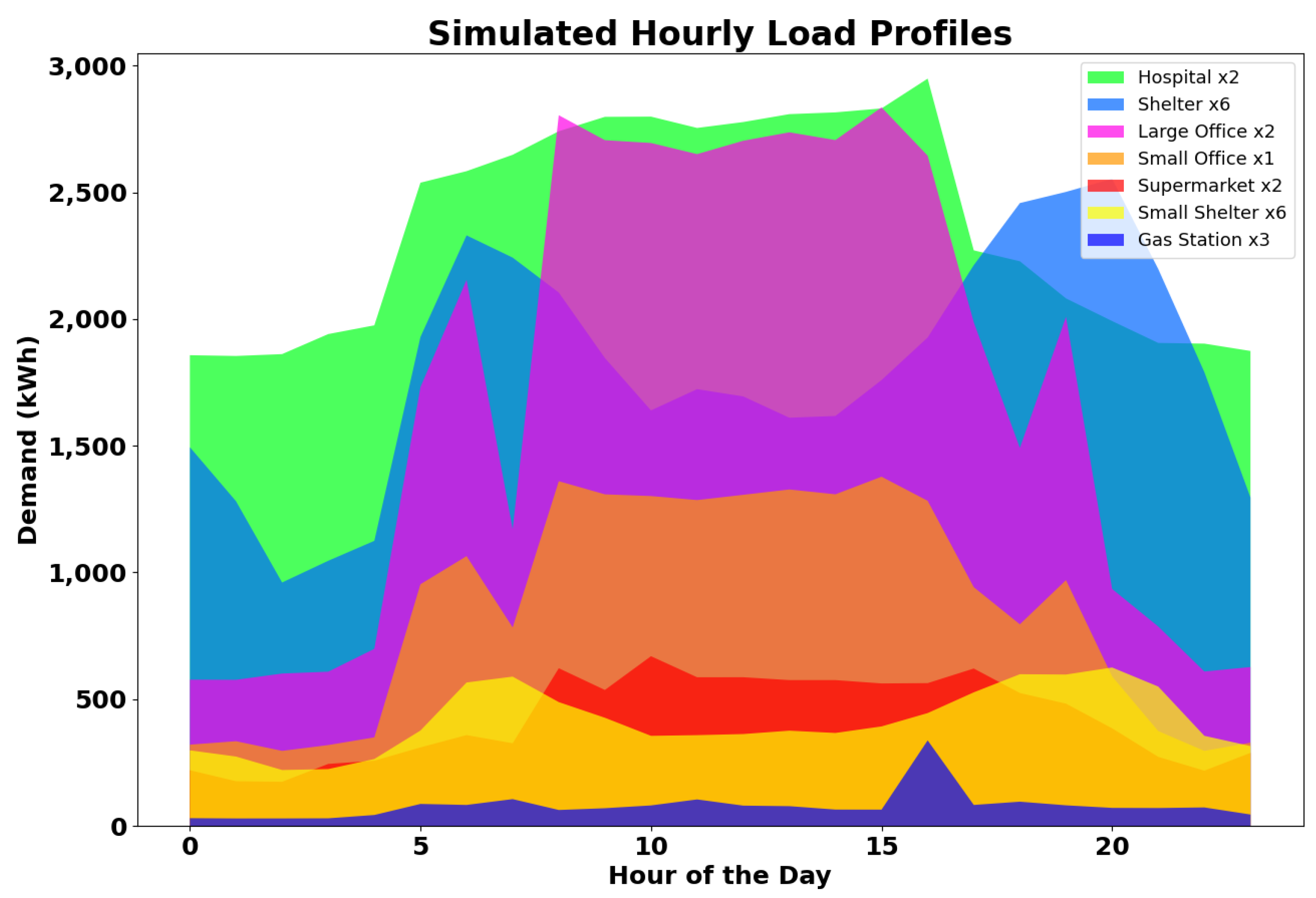
During the training phase of the RL-based energy management agents (EMAs) in simulation, the PV outputs and energy demands for all designated distribution nodes (DNs) are stochastically generated using the fitted distributions. This approach enables the modeling of environmentally dependent PV output (refer to Figure 1) and the stochastic nature of energy demands across different types of buildings (refer to Figure 2). For example, the energy demands of shelters exhibit peaks during the early morning and late evening hours, reflecting usage patterns characteristic of such facilities. Conversely, hospitals experience peak demand periods typically occurring in the middle of the day. By incorporating these stochastic elements into the simulation, the RL-based EMAs can effectively adapt to diverse demand profiles and environmental conditions encountered in real-world microgrid scenarios.
Figure 1 provides a visual representation of how PV output varies across different months. In January, which typically yields the lowest output, the available hours for PV energy production are reduced compared to July, the month with the highest energy output. Additionally, the peak outputs exhibit considerable variation across different times of the year. The Figure demonstrates that the fitted distribution generated outputs mimic the impact of environmental conditions on PV energy production present at different times of the year.
Figure 2 depicts the distinctive demand profiles of various loads throughout the day. Each load type exhibits unique patterns of demand variation over time. For instance, shelters show peak demand periods during the early morning and late evening, while hospitals experience peak demand in the middle of the day. These figures illustrate the dynamic nature of both PV output and energy demand, highlighting the need for adaptive energy management strategies in microgrid systems.

2.2. EMP as a Markov Decision Process

The challenge at hand can be formalized as a Markov decision process (MDP), aiming to derive the optimal EMS for the simulated DGMG. The objective is to achieve optimal cost-efficiency and demand coverage amidst uncertainties associated with renewable energy generation and grid disruptions.
In the MDP framework, defined by a tuple consisting of states S, actions A, transition probabilities P from one state to another, and immediate rewards R a for actions taken, the system’s state M t comprises variables representing various aspects: the current renewable energy generation based on the month m and time step t, denoted as P m , t , energy storage levels S t (state of charge), and energy demanded by assigned facilities D t .
At each time step, an agent selects an action representing charging, discharging, or idling of the ESS. This action, chosen in state M t based on S t , P m , t and D t , determines the ESS charge level for the next time step, thereby influencing subsequent actions available to the RL agent. Transition dynamics are influenced by the stochastic nature of P m , t , D t , and grid disruptions.
The projected PV energy output P m , t is modeled as a distribution based on month, time of day, and unit size (Equation (1)). Similarly, energy demands D t of assigned facilities are modeled as a distribution linked to different times of day (see Equation (2)). These distributions characterize the probability of PV output meeting or falling short of projected energy demands (high scenario labeled H) or being insufficient (low scenario labeled L).
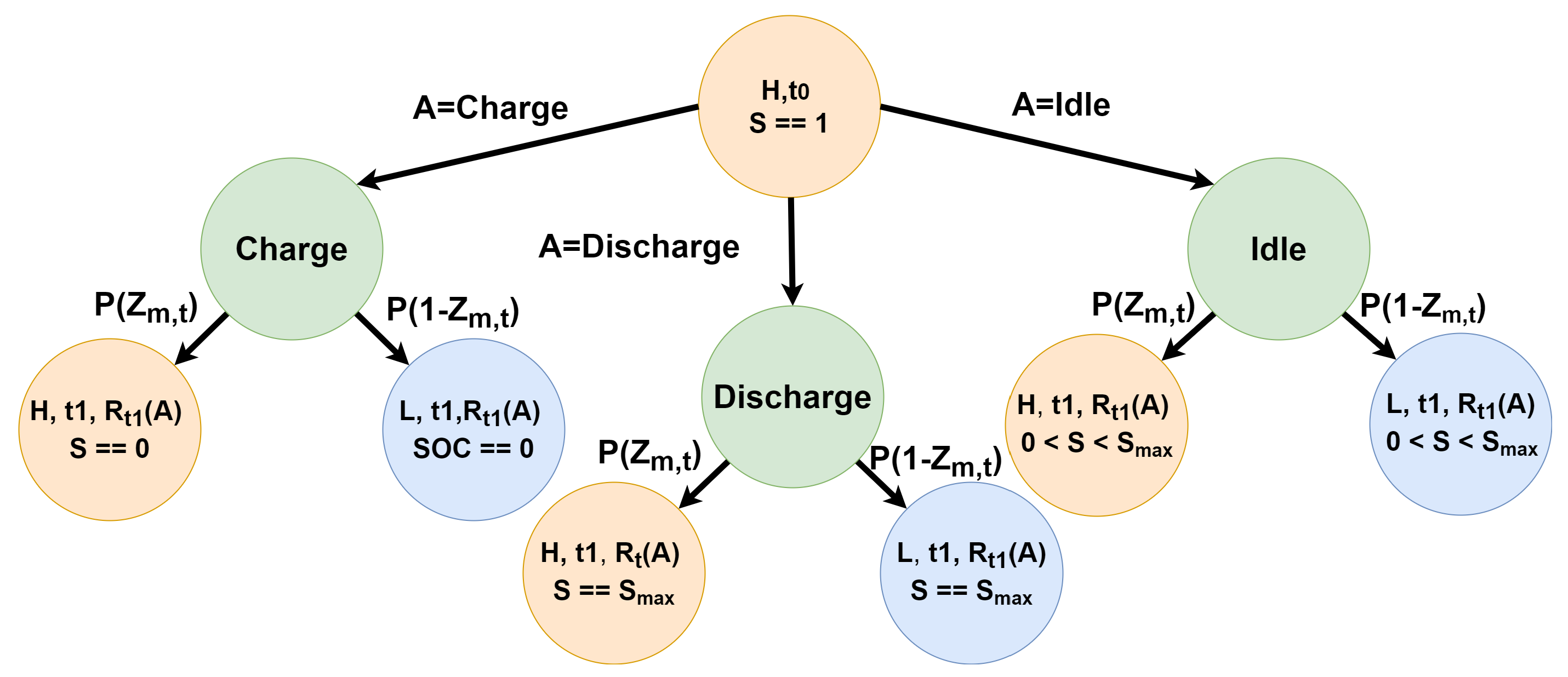
The subsequent state of the MG, concerning its ability to supply supplemental energy or store excess energy, hinges on the action taken at the start of the current state t 0 , affecting the ESS state of charge for the next state t 1 . Constraints dictate that if the ESS is fully discharged ( S = S m a x ) or fully charged ( S = 0 ), it can only charge or discharge in the following state, respectively. The action chosen in any state, along with the probability Z m , t of high PV output, determines the next state of the system (Equation (3)), illustrating a Markov process where actions in the current state influence subsequent states.
P m , t { P | m , t , p d f t , m }
D t { D | t , p d f t }
Z m , t = P ( P m , t D t )
When modeling the process as a Markov chain decision tree (see Figure 3), each node labeled H or L denotes the beginning of an hour during which the ESS unit undergoes charging, discharging, or remains idle based on the chosen action. At each node, there exists a probability Z h representing whether the PV output is sufficient to meet demand or falls short. In cases where demand exceeds PV output, power must be procured from the grid at a cost or supplemented using the ESS unit to bridge the gap between supply and demand. Conversely, when the PV and ESS units’ combined output exceeds demand when discharging, the surplus can be sold back to the grid for a marginal profit.
The decision on how to operate the unit hinges on the state of charge (S) at the time of decision making, as depicted in Equation (17) described in Section 3. The overarching objective is to derive an optimal policy that recommends actions in a given state, maximizing not only the reward in the subsequent state but also the cumulative rewards across all future states. While tools like mixed linear and stochastic programming can address such problems, they have inherent limitations.
As depicted in the figure, the complexity of modeling increases exponentially with the number of time steps or stages considered. For each time step scenario pair, there are two potential new grid states, labeled as H and L, at each node. Equation (4) illustrates how the number of nodes | N | or stages to be modeled and solved using methods like stochastic programming grows with the time horizon T. For short planning horizons, such as 1 or 2 h, the number of nodes remains manageable, with only 3 and 7 nodes, respectively. However, when attempting to model a single day for an hourly energy management system (EMS), the number of nodes exceeds thirty-three million, rendering the problem intractable. This scalability issue limits the feasibility of long-term modeling using tools like linear or stochastic programming.
In contrast, RL solutions do not suffer from this scalability limitation and can provide optimal policies over large time windows by leveraging adequate models and simulations of the systems to be optimized. RL operates within the framework of MDPs and employs machine learning techniques to discover optimal policies without requiring explicit formulation. These aspects of RL methods make them well-suited for complex, uncertain problem optimizations.
The subsequent section delineates the two RL methods employed in addressing the energy management problem in this study and elucidates how RL methods are grounded in the MDP framework.
| N | = t T 2 t Number of Nodes as a function of time horizon T

2.3. A2C and PPO Reinforcement Learning Optimal EMS

RL is a form of machine learning that learns in a manner similar to how biological organisms learn through interaction with their environment. RL consists of the learning agents having experiential episodes of some task for which they are to produce an optimal policy, which provides the action to take based on the state of the system. The agents store sample state, action, and reward experiences within a limited memory and utilize these “memorize” in a stochastic mini-batch manner to learn. The learner must discover the appropriate actions to take in an environment to maximize some future reward provided by the environment due to the action. The goal is to learn the optimal mapping of states to action or the optimal policy. Reinforcement learning requires a formulation following the MDP framework consisting of the environment, a method of describing potential states the environment can take, a set of actions an actor can take to affect the state of the environment, and some function that determines the values related to states, or states and action pairs based on some reward. The reward is some value that indicates the improvement or deterioration of the state or the achievement of some objective. Objectives such as playing video games, moving robots in more naturalistic manners, and even large language models utilize RL to great success. The following sections will provide brief descriptions of the basic concepts of RL and the two methods of DRL utilized in the work.
There are various methods, such as dynamic programming or temporal difference RL, that are value-focused. Methods such as these focus on approximating the values of specific states or state-action pairs based on the returns of some series of actions. The application of deep learning allows for deep reinforcement learning and policy gradient methods that seek to estimate the policy directly. Policy gradient methods use the tool of gradient descent to estimate the probability of each action leading to the greatest return in the current state. The methods used in these works, A2C and PPO, are a combination of both. Both methods use a dual network structure where one network is trained to produce a probability distribution that, when an input state is provided, indicates the probability of each action leading to the largest future return, and another that “critics” the advantage gained from the action taken by the former network by estimating the value of the resulting state.
This network structure helps to alleviate a few of the harder-to-handle aspects of DRL. First, due to the experiential nature of RL, the learning agents may attain misrepresentative or misleading sample data with which to learn. DRL consists of the learning agents having experiential episodes of the task for which they are to produce optimal policy. The agents store sample state, action, and reward experiences within a limited memory and utilize these “memorize” in a stochastic mini-batch manner to learn and update their weights to relate which set of probability estimates to produce for the potential actions that indicate which actions to take to achieve the optimal future return. This future return can be at the end of some overall task or some finite set of future rewards indicated by the discount factor. The discount factor controls how much attention the agent pays to the future rewards for a given action. These data can lead to the RL agent “learning” bad policy behaviors that, when applied to the bad samples, produce optimal future returns or the sum of future rewards but produce suboptimal results when applied to the general system.
The reinforcement learning algorithms used in this work are the A2C and the PPO algorithms. The A2C network is a type of RL architecture that combines elements of both value-based methods and policy-based methods. As the name suggests, two components of the network structure are linked in the gradient learning step of the algorithm. The “actor” component of the network is what provides the policy by learning the probability estimate for the actions (discharge, charge, idle) leading to the greatest future reward. The goal of the actor is to find an optimal policy π such that in any given state s it will provide the action most likely to lead to the greatest return. In this formulation of the problem, the return reward for a given action is the current cost/profit in the connected scenario, and the amount of demand met in the islanded case.
The “critic” component evaluates the actions chosen by the actor by estimating the value function (Equation (5)) for the state value produced by the action. The value function represents how good a particular state is in terms of expected future rewards. The goal of the critic is to help the actor learn by providing feedback or critiques on the chosen actions.
v π = E π [ R t + 1 + γ v π ( S t + 1 ) | S t = s ]
When training an A2C network, the actor and critic are updated based on the rewards for actions and state value estimates obtained from interactions with the environment. The critic provides a temporal difference (TD) error signal, which indicates the difference between the predicted value of a state and the actual observed value of a resulting state due to an action. This error is used to update the critic’s parameters, typically using gradient descent methods to adjust the predicted likelihood of the action, leading to greater returns. For the actor, the policy is improved using the critic’s evaluations. During training, the actor will begin to prefer actions that lead to higher estimated future rewards, according to the critic.
Like in other RL methods, actor–critic networks face the challenge of balancing exploring new actions to discover potentially better ones and exploiting current knowledge of the best-known or experienced actions. This balance can be achieved through exploration strategies or techniques like adding exploration noise to the actor’s policy by adding some randomness to the actions taken during training. This work uses the policy as a probability of action selection during training to allow for exploration, and a deterministic max value selection method after. Actor–critic networks often see faster convergence compared to pure policy gradient methods because they learn both a policy and a value function. The value function provides a more stable estimate of the expected return, which can guide the actor’s learning process more efficiently.
PPO is a popular reinforcement learning algorithm known for its stability and robustness in training neural network policies. PPO belongs to the family of policy gradient methods, which directly optimize the policy function to maximize the expected cumulative reward. PPO aims to improve the policy while ensuring the changes made to the network during training are not too large, which could lead to instability. To achieve this, PPO introduces a clipped surrogate objective function. This objective function constrains the policy updates to a small region around the old policy, preventing large policy changes that could result in catastrophic outcomes. The RL agent could adjust the weights in a drastic manner, leading to the agent becoming trapped in local optima. PPO offers several advantages, including improved stability during training, better sample efficiency, and straightforward implementation compared to other policy gradient methods. By constraining the policy updates, PPO tends to exhibit smoother learning curves and is less prone to diverging or getting stuck in local optima. PPO can be used along with actor–critic architectures as described above which is the methodology taken in this work.
In actor–critic with PPO, the actor’s policy is updated using the clipped surrogate objective, ensuring that the policy changes are within a safe range. The critic’s role remains the same, providing feedback to the actor based on the estimated value of the state arrived at due to actions. The stability of PPO combined with the value estimation of actor–critic architecture allows for the leveraging of the advantages of both approaches. This hybrid approach often leads to efficient and stable training of neural network policies in reinforcement learning tasks. Four total RL networks were trained and tested for this work to analyze if grid-connected only or connected with intermittent monthly disruptions allow for more disruption-resilient policies. The networks have slightly different reward structures based on the scenarios they are trained. The always fully grid-connected model focuses on maximizing daily energy cost coverage while meeting maximal demands. The reward function for the two grid-connected trained networks (PPO-G, A2C-G) uses the hourly cost of purchasing or profit from the sale of energy of on and off-peak energy costs based on the utility company. In contrast, the networks trained with intermittent disruptions have a modified reward structure that considers cost when connected and focuses solely on demand when in an isolated state.
The RL networks for this work are coded in Python (v3.9) using PyTorch (v2.2.1) and utilize an AnyLogic (v8.8.6) simulation of an MG for training and testing. The simulation models the MG at the hour level with the EMS agents being tasked with providing an action for the ESS unit to take (charge, discharge, idle) over the hour based on the current state. To train the networks, simulations run for a total of 72 months. During each simulation, the months are treated as episodes, and the two RL models had the network layers, sizes, learning, momentum, and learning decay weights tuned through experimentation.

2.3.1. EMP as an RL Formulation

Formulating the EMP as an RL problem entails treating the energy grid as the environment, comprising both the MG and the main utility. The state of the environment reflects the dynamics of the MG, encompassing interactions among energy sources and loads. In the EMP context, actions pertain to operations affecting the ESS, while the reward corresponds to energy costs or profits resulting from these actions, or the overall load coverage depending on the chosen objective. Optimal action selection depends on the current MG state, influenced by the probabilities of energy output levels ( P ) and demanded loads ( F ) for a given hour h.
The RL agent learns from experience gained by operating the ESS within this environment. In this work, a simulation is developed to replicate the energy grid, comprising distributed generation units comprising solar power generation and energy storage systems. The energy grid model is conceptualized at a high level, focusing on simplifying energy interactions. Emphasis is placed on exploring capabilities, training strategies, and policies, particularly in scenarios involving connectivity uncertainty and inherent uncertainties in renewable energy generation and load demands.

2.3.2. Training and Tuning the RL Networks

The PPO and A2C models are tested with two training methods. First, the two methods (PPO-G, A2C-G) are trained in only a grid-connected scenario where the option to buy energy from the grid is always available. This scenario assumes a buyback program where any excess energy produced by the DG unit is sold back to the grid for a profit. The next two models (PP0-D and A2C-D) are trained in a simulation where there is a one in four chance each hour of a month that a seven-hour outage will occur. If the outage occurs during the month, no other outages will occur during that month. Each model is given a total of 72 months of training.
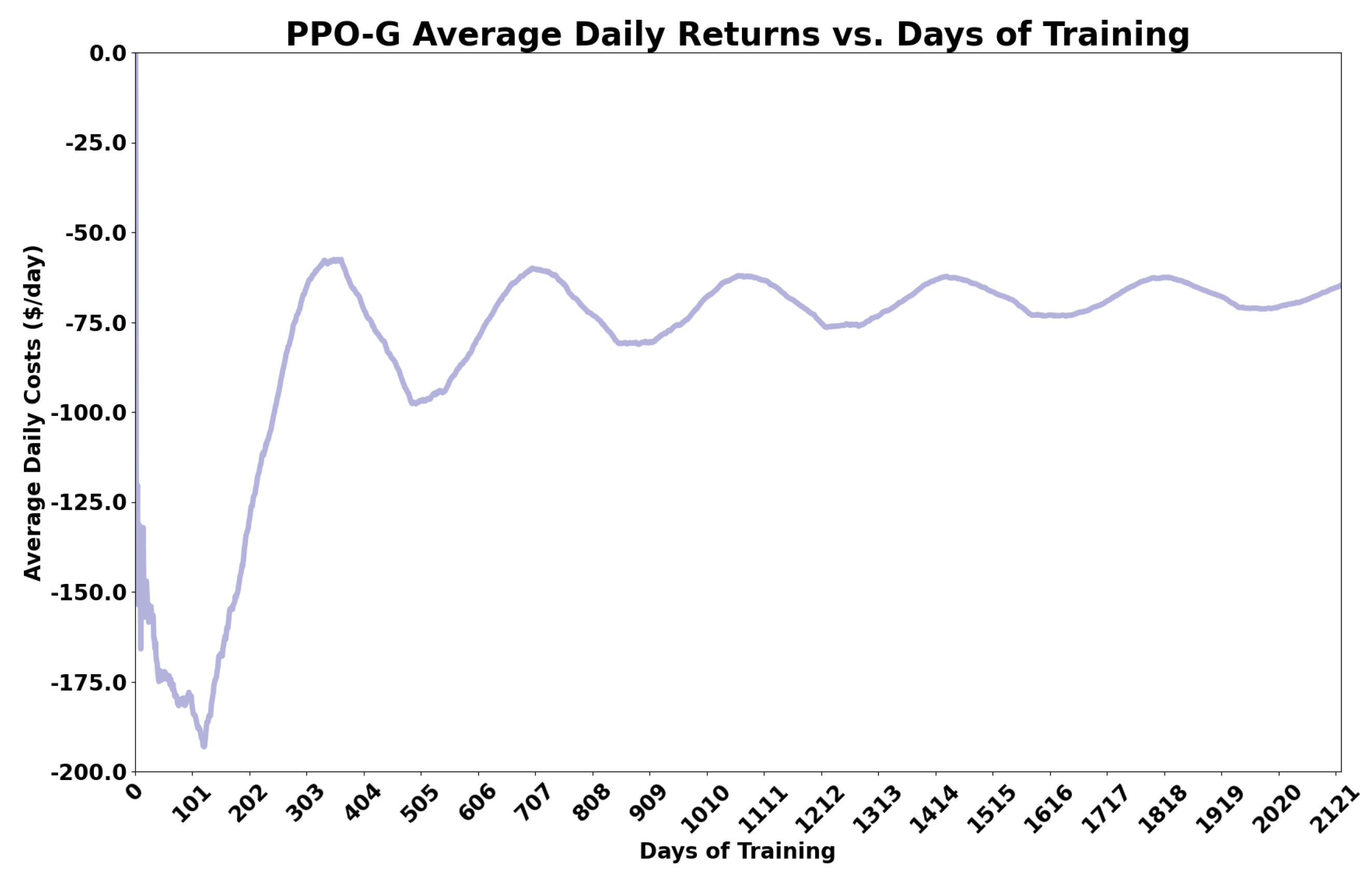
The training and testing of the models are performed using a simulation developed in AnyLogic as described above. The RL agents are tasked with providing ESS actions at the beginning of each hour of the simulation. A learning interval is set so that after a set number of episodes or months for this problem, the learner uses the experience to optimize the policy and state advantage estimations to find the optimal EMS. Various network structures, learning intervals, and hyperparameter settings were explored to find those that allowed the models to learn. Figure 4 shows a visualization of the PPO grid-connected, or PPO-G, trained model average cost returns over the course of 72 training months.

2.4. Baseline Comparison Methods

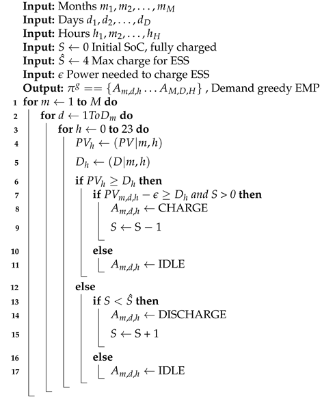
The RL-derived EMS are bench-marked against a heuristic algorithm designed to prioritize demand fulfillment and a randomized ESS operation simulation. This heuristic algorithm permits charging only when the charging of the ESS unit will remove the DG unit’s ability to meet demand, and discharging occurs solely when the expected PV output for the hour is less than the demand. The pseudocode for the greedy algorithm is depicted in Algorithm 1. In the test case, a 38 MW PV unit with a collocated 8 MWh lithium ion battery ESS serves as the distributed generation (DG) system.
Algorithm 1: Demand Greedy EMP Algorithm
Energies 17 02821 i001
The following section mathematically formulates the cost- and demand-coverage problems as maximization problems.

3. Problem Description and Formulation

The sets, variables, and parameters used to describe the model can be found in Table 1, Table 2 and Table 3. The problem consists of a distributed generation unit consisting of unit a PV unit P and co-located lithium-ion energy ESS E to provide power for a selected set of facilities F within a grid-connected microgrid.
The EMA aims to maximize the MG’s energy autonomy by minimizing the amount of energy purchased from the utility, indicated by a negative T m , h value, while maximizing the profits from selling any excess energy back to the grid, indicated by a positive T m , h value, (Equation (6)) in a grid-connected scenario. Positive T m , h values indicate a profit and negative values indicate an energy cost of purchasing power. However, during a service disruption from the main utility, the EMA objective becomes maximizing the amount of power supplied to the facilities T m , h with Equation (7), which no longer takes into account the ability to sell excess energy back or the cost of purchasing energy since the grid is not available.
max m = 0 M d = 0 D m h = 0 23 T m , h × B h | M |
max m = 0 M d = 0 D m t = 0 23 T m , h | M |
Equation (8) defines the total power supply available from the DG unit for a given month and hour. Additionally, Equations (9) and (10) specify the constraints on the output of the PV and ESS units, respectively. The ESS output during hour h due to action a, denoted as E h , a , is subject to limitations based on both the SoC represented as the number of consecutive discharges C h of the ESS at the beginning of hour h and the action a h taken by the EMA. The ESS can not exceed the stated number of consecutive discharges Δ without a charge (Equation (11)). Equation (12) determines the ESS output over h based on C h and a h . The EMA is tasked with deciding when to discharge, charge, or keep the battery idle for each hour h. The ESS is designed to provide ϵ for four consecutive hours without requiring a recharge, but it demands one hour of charging for every hour of discharge to recharge the battery, as indicated by Equation (12).
S m , h = P m , h + E h , a
P m , h ρ
E h , a ϵ
0 C h Δ
E h , a = ϵ if a = 0 & C h < μ ϵ λ if a = 1 C h > 0 0 otherwise
The set of facilities consists of different buildings, each with varying energy profiles over the course of a day (see Figure 2). The total demand over an hour h is determined by Equation (13), and thus, the difference between the expected load L h and supply S m , h determines if there is a cost for buying power or profit for selling excess power (Equation (14)). When T m , h is negative, supplemented power must be purchased from the grid at the current cost of energy B h , and when it is positive, the ability to sell the excess energy back to the grid arises.
L h = f = 0 F δ f , h
T m , h = S m , h L h
The reward for the time step is the energy cost or profit incurred due to the difference in the total supplied power S h and demand D h , T h , with Equation (8). The hourly costs or profits are the product of T m , h and the cost of energy over the hour h calculated with Equation (15). This value will be negative if the demand exceeds the energy supply and positive (profit) otherwise. This reward trains the EMA to utilize the ESS in a way that will lead to minimized costs and maximal profits over the course of the training. However, some steps must be taken to ensure that the EMA does not just discharge the ESS during high times of PV output since this would contradict the role of good energy management by potentially leading to excess reverse power flow and system damages while not supplying the load during low-cost times. The return for an episode, a month in this case, is the summation of all rewards over the course of a given month with Equation (16). It should be noted that factors such as investment, operating, and maintenance costs and efficiency losses are not included in the model. This is because this work focuses on the ability of the employed methods to optimize cost and demand coverage across diverse scenarios.
R h = B h × T m , h
G m = d = 1 D m h = 1 23 R h
To ensure that the EMA will not “learn” a bad EMS that allows for infeasible operation, an action filter is employed that restricts the action options based on the MG state (Equation (17)). The possible actions over hour h are dependent upon the SoC C h of the ESS, P m , h , and D h expected over an hour. The actions available to the EMA dictate the potential states. The action taken over a given time step directly influences the following state be influences the resulting SoC of the ESS unit. This subject leads into a description of EMP as a Markov decision process, discussed next.
α h { 1 , 0 , 2 } , 0 C h N a b s ( P m , h D h ) < ϕ { 0 , 2 } , C h = = Δ T m , h < D h { 1 , 2 } , C h = = 0 P m , h > D h { 2 } , o t h e r w i s e

3.1. Analytic Methods

The study compares the objectives of energy cost coverage in a grid-connected scenario, energy demand coverage in an islanded scenario, and intermittent disruption scenarios using two reinforcement learning methods for the agents. The performance of the RL agents across the scenarios is compared alongside a randomly operated EMS and a demand-focused heuristic algorithm. To compare cost coverage, the average daily percentage of the normal costs reduced by the use of the derived EMS is calculated in the grid-connected scenario. The goal in grid-connected scenarios is to maximize the average daily energy cost coverage by the DG unit and the operation of the ESS. This is measured as the percentage difference between the average costs without using an ESS and the average daily costs when employing one of the derived EMS. The calculation involves taking the ratio of the average energy costs for the derived EMS to the average daily costs, subtracting this value from one to determine the percentage of costs covered. Specifically, the comparison is between the average daily costs incurred without an ESS (C) and the average daily costs using the EMS derived by one of the tested methods ( C ^ ). In this scenario, costs can reflect either profits from selling excess energy back to the grid or expenses from purchasing energy when the DG unit cannot meet demands. (see Equation (18))
% of   Average   daily   energy   cost   overage = C C ^ C
In contrast, the average percentage of hourly demands covered by the DG unit through the EMS are compared in the islanded and intermittent disruption scenarios. This comparison aims to assess the effectiveness of each method’s derived EMS policy in optimizing objectives across scenarios. The calculation consists of the ratio of the difference between the average energy demands supplied D with no ESS and the average daily demands supplied using the different EMA methods D ^ over the original average daily demands supplied D (see Equation (19)).
% of   Average   daily   demand   overage = D D ^ D
In addition, an analysis and comparison of the policies generated by the RL agents is performed to explore what types of energy management strategies (peak shaving, profit generation) the models are employing.
The A2C and PPO EMAs were each trained using the AnyLogic simulation to provide experience, and several rounds of hyperparameter tuning were performed to find the optimal configurations. The average monthly energy costs and average monthly demand supplied are compared and analyzed to compare the performance of the three EMAs. In addition, the different charging strategies produced by the EMAs are analyzed for voltage regulatory or peak demand shaving behavior. The subsequent section describes the model configuration and parameters.

3.2. Model Configuration

The test case the EMAs were tested on consisted of a 50 MW PV unit and a 32 MWh (8 MW/h) ESS unit assigned to an MG containing two hospitals, two supermarkets, four gas stations, two large office buildings, a small office building, six large housing facilities, and six small housing facilities. The average demand for the twenty-one DNs is around 7 MW daily. The ESS capacity is chosen to cover the average demand. Similarly, the PV unit is chosen to cover the peak demand and provide enough excess energy to charge the ESS without hurting its ability to meet demand at peak output times. The test simulation of the MG is tested with three scenarios. First, the EMAS must optimize the average monthly costs and demands met over a four-year simulation without disruptions. Second the agents must provide optimal EMS in an island mode scenario, Lastly, the simulation induces stochastic disruptions that isolate the MG from the main utility forcing the DG to provide all power for the MG. The following section details and compares the results for each EMA and analyzes the behavior of the energy management strategies produced.

4. Results Discussion

4.1. Grid Connected Cost Coverage and Demand Coverage

The results for the average daily percentage of cost and demand covered by the tested EMS methods can be seen in Table 4. Compared to randomly generated and energy demand-focused EM methods, both RL-derived solutions show the highest percentages of cost covered. Utilizing the ESS unit randomly allows for around 44% of the average daily energy cost. When discharging, whenever the solar output cannot meet demand and the ESS is in a state where it can do so allows for around 59% of the average daily costs. In contrast, the A2C and PPO methods trained with only grid-connected scenarios covered 86% and 83% of the daily costs, respectively. When trained with intermittent monthly disruptions, the performance falls to 69 and 51 percent for the A2C and PPO methods, respectively. This indicates that when only trained to meet demand in an islanded scenario with only the PV unit to charge, the learners have a much more difficult time finding the optimal policy for a new unseen scenario. Interestingly, the PPO method still outperforms the greedy method’s ability to cover the daily energy costs, meeting almost 70% of daily costs. In contrast, the AC model falls below the performance of the greedy method.
Comparing the demand covering ability of the methods, the grid-connected trained RL methods again perform the best, but the magnitude of the improvement is less compared to the greedy method. The demand-focused algorithm allows for 53% of daily energy demands to be covered by the DG unit. An almost ten percent improvement in daily demand coverage is seen for the PPO-G and A2C-G methods, with them covering 61% and 62%, respectively. The RL methods trained in isolation now match the greedy algorithm’s performance. These results signal that the demand coverage capabilities of the PPO and A2C methods trained with grid-connected scenarios are more similar than their cost-covering abilities. The A2C method even slightly outperforms the PPO in this metric.
The result shows that RL can be utilized to find maximal solutions for mitigating energy costs and meeting demands. The cost and demand coverage results also indicate that when trained to focus only on the daily operation of the PV unit and only allow for the PV unit to charge the ESS, the RL can learn policies that can outperform a purely demand-focused heuristic but are still outperformed by models that are trained with the options of buying energy from the grid to charge the ESS and attempting to meet demands outside of the sunlight hours when the PV unit can produce. However, increasing instabilities and stresses on the energy grid due to increasing renewable penetration will inevitably lead to increases in disruption. The following section compares how well the trained agents perform in a simulated island mode situation where the goal is to provide high-demand fulfillment when the DG unit is the main source of energy for the ESS.

4.2. Island Mode Performance

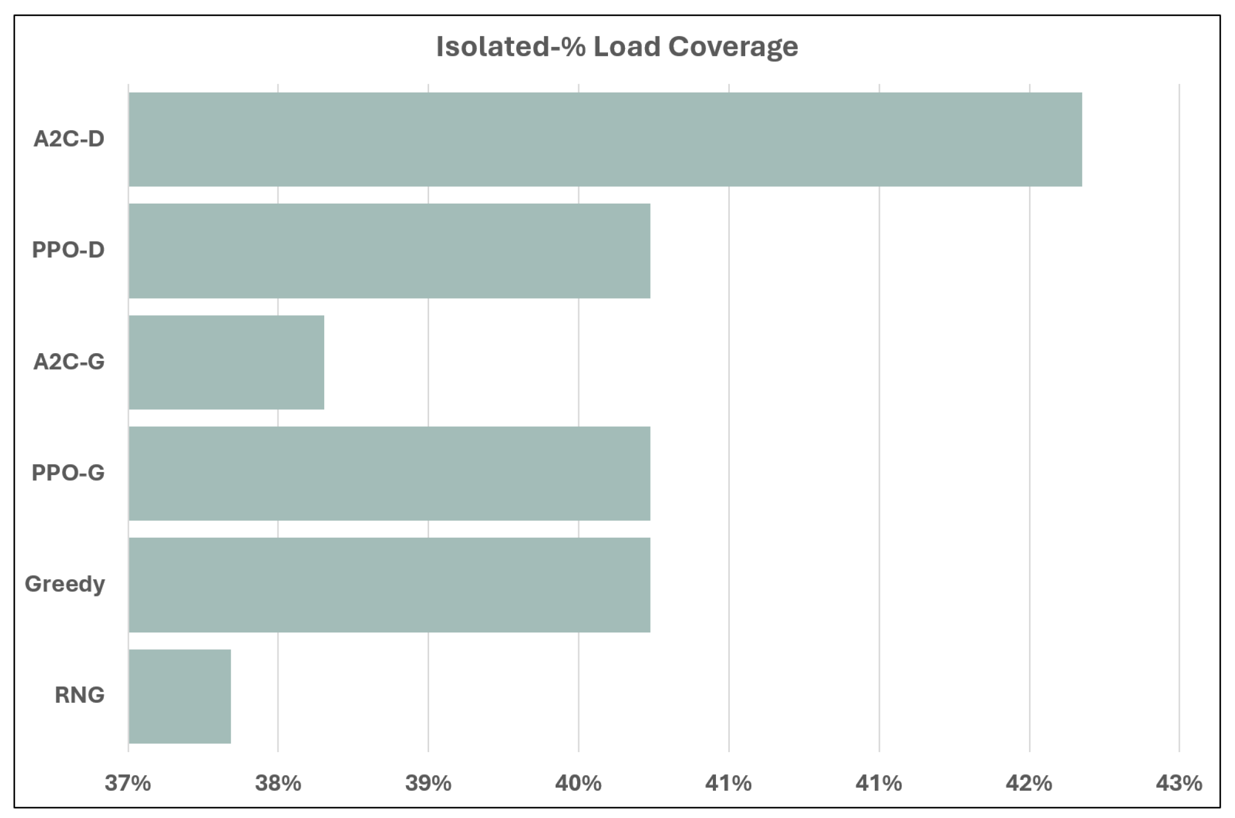
Figure 5 shows the average daily percentage of energy demand coverage across all demand nodes by the tested EMS methods. In contrast to the objective of cost coverage in a grid-connected case, when the cost is no longer a factor due to the only energy source being the PV unit, A2C allows for better demand coverage than the PPO EMS. The A2C can almost cover 100% of average daily demands compared to only 41% for the PPO-derived EMS. The result indicates that while a given EMS derived from an RL agent trained for a grid-connected scenario performs well, there is a need for the EMS method to be robust in island situations. A middle ground should be sought so that derived EMS allows for profit and is resilient to disruptions. Steps should be taken to ensure the robustness of RL-derived EMS strategies that can encompass the potential state of the MG.

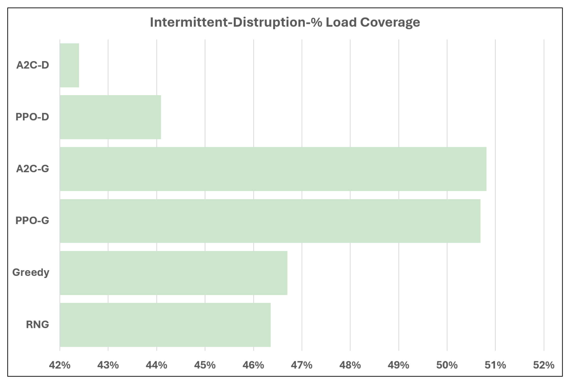
4.3. Intermittent Disruptions

The final set of tests tasks the methods with optimizing demand coverage with randomized week-long disruptions each month of the testing. The results are displayed in Figure 6. When tasked with providing demand coverage when the energy grid connectivity is uncertain, the grid-connected trained models vastly outperform the other methods. For the intermittent connectivity issue scenario, the models trained with disruptions perform starkly worse than in the isolated case where they are at the upper end of load coverage capability. It seems that the models trained only on grid-connected scenarios do a good job of handling the few hours a month where the grid connection fails. In contrast, the models trained with intermittent disruptions match or exceed the performance of the former methods at handling the isolated scenarios, with the A2C-D method outperforming all others.

4.4. Analysis and Comparison of RL EMS Policies

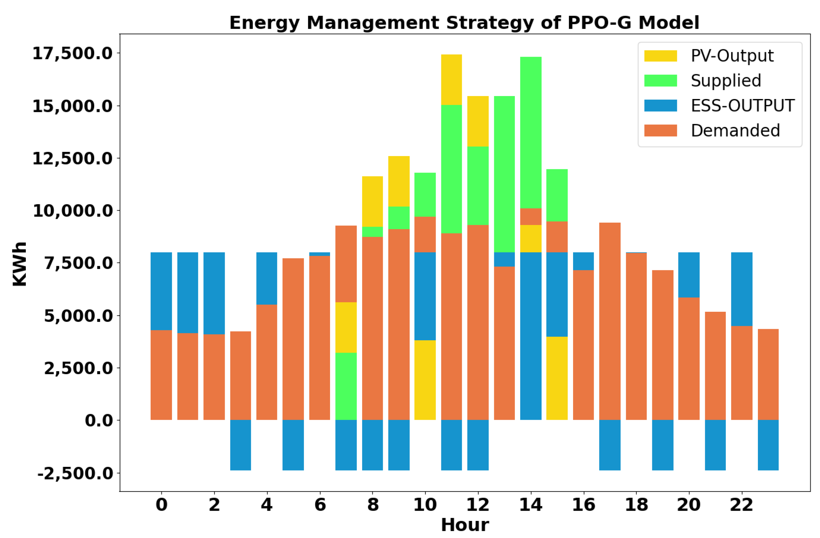
During each simulation, the energy output of the PV and ESS unit is tracked alongside the energy demands at each hour and the costs or profits generated. Analyzing the discharging and charging behavior exhibited by the RL agents can provide insights into the logic, if any, behind the learned policies. Figure 7 visualizes the energy output for the ESS and PV units, the total supplied energy from the two sources, and the energy load for each hour of a simulated day based on the policy derived from the PPO-G model. Hours with the top color in blue, such as hours 0–2, indicate that the ESS unit is the sole energy source, discharging and supplying more than needed. When the green bar is at the top, the combined power from the ESS and PV units is more than sufficient to meet energy demands. If the yellow PV bar is above the green bar, it signifies that the ESS is being charged by the PV unit, thereby reducing the total energy supplied. In a grid-connected scenario, the EMS model allows the ESS to provide supplemental energy outside sunlight hours, charge during sunlight hours, and generally meet demands. It also generates the most excess energy during peak PV output hours, producing profits for every kWh exceeding demand. During the pre-sunlight and post-sunlight hours, the model utilizes the ESS in varying ways (blue top bars). The early morning hours between midnight (hour 0) and 6 AM show that the model had stored enough energy to provide three consecutive hours of load coverage, with the following intervals of charging and discharging. This behavior provides as much constant energy as possible until the ESS is depleted, followed by alternating actions to provide some load coverage whenever the ESS is able to. Once the PV can provide energy after 6 AM, the PPO-G-based policy sees the ESS mostly either charging consecutively (blue bottom bars) at no cost using the PV unit or providing supplement energy during the tenth and thirteenth through fifteenth hours. It should be noted that the peak demand and energy cost hours are between the fourteenth and twenty-first hours of the day. Looking at the figure, it can be seen that this is when the most consecutive discharges occur, leading to the required load being exceeded by the energy supplied, leading to the highest potential profits. From these results, it seems that the model learns to store energy consecutively during the sunlight hours while preferring to charge cyclically when the cost-free energy provided by the PV unit is unavailable. In addition, the model seems to prefer achieving profits by providing excess energy during peak energy price times based on the availability of PV energy. Thus, the policy produced by the PPO-G model can provide decent load coverage during the low sunlight hours while also providing actions that provide profits that help offset the costs incurred when the PV energy output is insufficient.
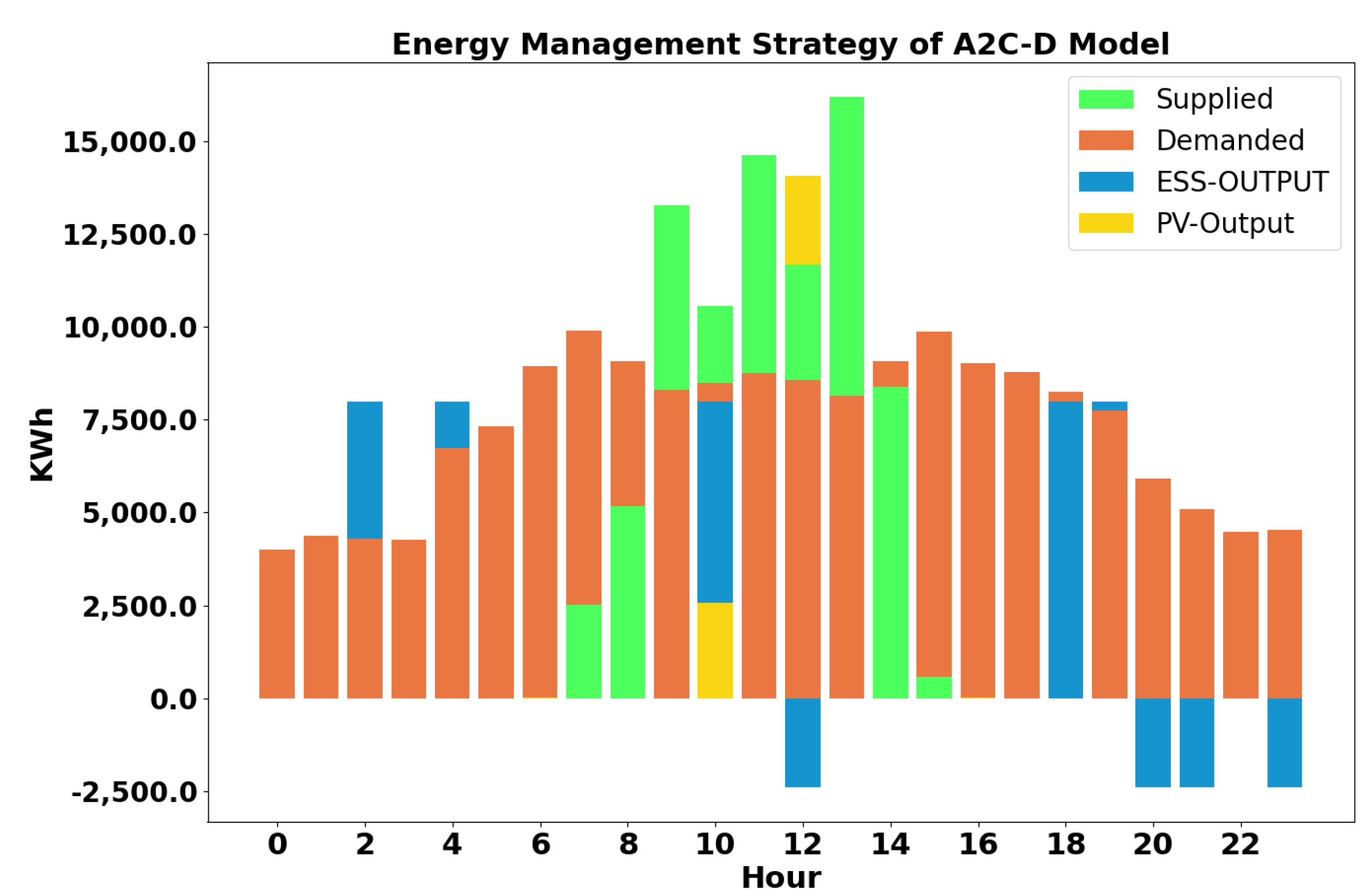
For the A2C-D model, which has the highest performance in isolated scenarios, Figure 8 shows an example of the policy over a twenty-four hour period in an isolated scenario. This model’s reward function focused on maximizing demand with no consideration of cost. Areas, where orange is the top color, indicate hours where some amount of power proportional to the size of the orange space could not be met. The larger the orange part of the bar, the larger the amount of unmet demand. In contrast, areas where either the blue bar representing only ESS output, or the light green supply bar representing the summation of ESS and PV output are on top represent hours where the energy supplied by the DG unit was at least sufficient to meet load demand.
From Figure 8, the ESS is utilized mostly outside of maximal PV generation hours (blue bars at hours 2, 4, 18, and 20). This policy sees charging during the early morning and later in the evening, leaving the PV unit to provide power during the sunlight hours. The EMS allows the PV unit to provide energy during the sunlight hours; charging only when doing so still allows for demand to be met by the remaining PV output (see hour 12), and discharging only when the PV unit can not provide sufficient power over the hour on its own (see hour 10) or when there is no energy provided by the PV unit (see hour 2 and 4). Since the cost influences at on and off-peak times are not a factor for this model, there is no effort to add excess energy at peak energy price times. The focus is more on providing energy from the ESS as a supplemental energy source when the PV output is lacking.

5. Conclusions, Limitations, and Future Work

This work investigated the use of RL-based energy management agents trained under utility grid-connected, islanded, and grid-connection uncertainty scenarios. A model and simulation of a distributed generation microgrid (DGMG) connected to these three scenarios were developed. The best-performing energy management strategies were analyzed to understand the logic behind the derived action policies. The comparison focused on the ability to cover daily energy costs or generate profits from excess energy sales, as well as the average daily load demand met by the derived policies. This comparison was conducted across four RL networks trained under grid-connected and intermittent grid connectivity scenarios.
The simulation results showed that in grid-connected scenarios, the proximal policy optimization (PPO) and advantage actor–critic (A2C) networks trained in grid-connected simulations outperformed those trained with simulated grid connectivity disruptions. Both the grid-connected trained PPO and A2C networks were capable of generating energy management system (EMS) policies that maximize daily cost and demand coverage, with the PPO network meeting a higher percentage of energy costs and load demands on average. Additionally, these grid-connected trained RL networks performed best during intermittent grid disconnections in terms of average daily load demand coverage, with the A2C network demonstrating slightly better but comparable performance. However, in scenarios involving an islanded DGMG, the A2C network trained with utility grid connection uncertainty outperformed all other tested methods in terms of the percentage of daily demands supplied to the loads.
The results indicate that policies derived from the PPO model trained in a grid-connected simulation provide a higher rate of cost recovery and potential profit and demand coverage, but underperform in islanded scenarios where the sole energy source for charging the energy storage system (ESS) is the photovoltaic (PV) unit. In contrast, when isolated from the main utility or if the grid has uncertain grid connectivity, the A2C model trained with connection uncertainty and A2C trained with constant main utility grid connection had the best performance, respectively. These findings suggest that those seeking to utilize RL methods for energy management policy generation should either test the training of agents in varied grid connectivity scenarios with accurate representations of the system’s state or employ different agents tailored to each grid connectivity scenario to ensure robust solutions against disruptions.
Moreover, the results indicated that different aspects of the policies emerged when analyzing the energy management strategies produced by the highest-performing networks. The policy generated by the PPO network trained with a static grid connection enabled the ESS to supply energy intermittently throughout the day, as well as to provide extra energy during peak price hours, generating profit for the microgrid. In contrast, the policy from the best-performing model in islanded scenarios, the A2C model trained with grid disruptions, focused mainly on supplying energy during non-sunlight hours when the PV unit was unable to provide power.
There are several limitations to the current study. Firstly, this is a focused case study of a simulated PV-based microgrid using data specific to Knoxville, TN, and particular capacities for PV and ESS units. Focusing exclusively on PV renewable energy sources (RES) leads to solutions and conclusions based solely on this type of RES. Results will vary when utilizing different energy sources such as wind or hydro energy. The solutions and their optimality will change when modeling different areas with varying levels of solar irradiance. For example, Knoxville, TN, has approximately seven sunlight hours per day, allowing the PV unit to produce enough energy to make an impact. In contrast, states like California or Texas, where solar radiation and climate conditions permit much longer and higher magnitudes of energy production, will yield significantly different results.
The methodologies described in this study will be expanded in future research to address some of these limitations. Data modeling of different RES and areas with different climate conditions will be explored to examine the robustness of EMS across different energy resources and climate conditions. Efforts to examine RL networks trained under both grid-connected and isolated conditions. This will involve a comparison with networks trained exclusively for specific scenarios, determined by the grid’s connectivity status, to assess whether a single RL network can effectively manage both situations compared to an EMS that uses separately trained networks. Furthermore, previous work that utilized genetic algorithms (GA) for optimal sizing, placement, allocation, and EMS configuration will be advanced to incorporate these trained networks, evaluating their efficacy against traditional methods in optimizing microgrid configurations.

Author Contributions

Funding acquisition, X.L.; methodology, X.L. and G.J.; project administration, X.L.; software, G.J.; writing—original draft, G.J. and Y.S.; writing—review and editing, Y.S. and X.L. All authors have read and agreed to the published version of the manuscript.

Funding

This research received no external funding.

Data Availability Statement

The data presented in this study are available on request from the corresponding author.

Conflicts of Interest

The authors declare no conflicts of interest.

Abbreviations

DNenergy demand nodes or facilities
DGdistributed generators
ESSenergy storage system
EMPenergy management problem
EMAenergy management agent
EMSenergy management strategy
PVphotovoltaic generator
PVDGphotovoltaic distributed generator
PVDG/ESSco-located PVDG and ESS
MGmicrogrid
DGMGdistributed generation microgrid
ODGSPoptimal distributed generation sizing and placement
RPFreverse power flow
RESrenewable energy source

References

  1. Evans, A.; Strezov, V.; Evans, T.J. Assessment of utility energy storage options for increased renewable energy penetration. Renew. Sustain. Energy Rev. 2012, 16, 4141–4147. [Google Scholar] [CrossRef]
  2. Mardani, A.; Zavadskas, E.K.; Khalifah, Z.; Zakuan, N.; Jusoh, A.; Nor, K.M.; Khoshnoudi, M. A review of multi-criteria decision-making applications to solve energy management problems: Two decades from 1995 to 2015. Renew. Sustain. Energy Rev. 2017, 71, 216–256. [Google Scholar] [CrossRef]
  3. Das, C.K.; Bass, O.; Kothapalli, G.; Mahmoud, T.S.; Habibi, D. Overview Of Energy Storage Systems in Distribution Networks: Placement, Sizing, Operation, And Power Quality. Renew. Sustain. Energy Rev. 2018, 91, 1205–1230. [Google Scholar] [CrossRef]
  4. NREL. Distributed Solar PV for Electricity System Resiliency Policy and Regulatory Considerations. 2014. Available online: https://www.nrel.gov (accessed on 1 March 2024).
  5. Kenward, A.; Raja, U. Blackout Extreme Weather, Climate Change And Power Outages. Clim. Cent. 2014, 10, 1–23. [Google Scholar]
  6. Stenstadvolden, A.; Hansen, L.; Zhao, L.; Kapourchali, M.H.; Lee, W.J. Demand and Sustainability Analysis for A Level-3 Charging Station on the U.S. Highway Based on Actual Smart Meter Data. IEEE Trans. Ind. Appl. 2024, 60, 1310–1321. [Google Scholar] [CrossRef]
  7. Lee, S.; Choi, D.H. Reinforcement Learning-Based Energy Management of Smart Home with Rooftop Solar Photovoltaic System, Energy Storage System, and Home Appliances. Sensors 2019, 19, 3937. [Google Scholar] [CrossRef] [PubMed]
  8. Hosseini, S.M.; Carli, R.; Dotoli, M. Robust Optimal Energy Management of a Residential Microgrid Under Uncertainties on Demand and Renewable Power Generation. IEEE Trans. Autom. Sci. Eng. 2021, 18, 618–637. [Google Scholar] [CrossRef]
  9. Ali, S.; Khan, I.; Jan, S.; Hafeez, G. An Optimization Based Power Usage Scheduling Strategy Using Photovoltaic-Battery System for Demand-Side Management in Smart Grid. Energies 2021, 14, 2201. [Google Scholar] [CrossRef]
  10. He, X.; Ge, S.; Liu, H.; Xu, Z.; Mi, Y.; Wang, C. Frequency regulation of multi-microgrid with shared energy storage based on deep reinforcement learning. Electr. Power Syst. Res. 2023, 214, 108962. [Google Scholar] [CrossRef]
  11. Gilani, M.A.; Kazemi, A.; Ghasemi, M. Distribution system resilience enhancement by microgrid formation considering distributed energy resources. Energy 2020, 191, 116442. [Google Scholar] [CrossRef]
  12. Kuznetsova, E.; Li, Y.F.; Ruiz, C.; Zio, E.; Ault, G.; Bell, K. Reinforcement learning for microgrid energy management. Energy 2013, 59, 133–146. [Google Scholar] [CrossRef]
  13. Alhasnawi, B.N.; Jasim, B.H.; Sedhom, B.E.; Hossain, E.; Guerrero, J.M. A New Decentralized Control Strategy of Microgrids in the Internet of Energy Paradigm. Energies 2021, 14, 2183. [Google Scholar] [CrossRef]
  14. Cao, J.; Harrold, D.; Fan, Z.; Morstyn, T.; Healey, D.; Li, K. Deep Reinforcement Learning-Based Energy Storage Arbitrage With Accurate Lithium-Ion Battery Degradation Model. IEEE Trans. Smart Grid 2020, 11, 4513–4521. [Google Scholar] [CrossRef]
  15. Lan, T.; Jermsittiparsert, K.T.; Alrashood, S.; Rezaei, M.; Al-Ghussain, L.A.; Mohamed, M. An Advanced Machine Learning Based Energy Management of Renewable Microgrids Considering Hybrid Electric Vehicles’ Charging Demand. Energies 2021, 14, 569. [Google Scholar] [CrossRef]
  16. Suanpang, P.; Jamjuntr, P.; Jermsittiparsert, K.; Kaewyong, P. Autonomous Energy Management by Applying Deep Q-Learning to Enhance Sustainability in Smart Tourism Cities. Energies 2022, 15, 1906. [Google Scholar] [CrossRef]
  17. Quynh, N.V.; Ali, Z.M.; Alhaider, M.M.; Rezvani, A.; Suzuki, K. Optimal energy management strategy for a renewable-based microgrid considering sizing of battery energy storage with control policies. Int. J. Energy Res. 2021, 45, 5766–5780. [Google Scholar] [CrossRef]
  18. Li, H.; Eseye, A.T.; Zhang, J.; Zheng, D. Optimal energy management for industrial microgrids with high-penetration renewables. Prot. Control Mod. Power Syst. 2017, 2, 1–14. [Google Scholar] [CrossRef]
  19. Eseye, A.T.; Zheng, D.; Zhang, J.; Wei, D. Optimal energy management strategy for an isolated industrial microgrid using a Modified Particle Swarm Optimization. In Proceedings of the 2016 IEEE International Conference on Power and Renewable Energy (ICPRE), Shanghai, China, 21–23 October 2016; IEEE: Piscataway, NJ, USA, 2016; pp. 494–498. [Google Scholar]
  20. Contreras, J.; Losi, A.; Russo, M.; Wu, F. Simulation and evaluation of optimization problem solutions in distributed energy management systems. IEEE Trans. Power Syst. 2002, 17, 57–62. [Google Scholar] [CrossRef]
  21. Tenfen, D.; Finardi, E.C. A mixed integer linear programming model for the energy management problem of microgrids. Electr. Power Syst. Res. 2015, 122, 19–28. [Google Scholar] [CrossRef]
  22. Tabar, V.S.; Abbasi, V. Energy management in microgrid with considering high penetration of renewable resources and surplus power generation problem. Energy 2019, 189, 116264. [Google Scholar] [CrossRef]
  23. Singh, U.; Rizwan, M.; Alaraj, M.; Alsaidan, I. A Machine Learning-Based Gradient Boosting Regression Approach for Wind Power Production Forecasting: A Step towards Smart Grid Environments. Energies 2021, 14, 5196. [Google Scholar] [CrossRef]
  24. Zhang, B.; Hu, W.; Xu, X.; Li, T.; Zhang, Z.; Chen, Z. Physical-model-free intelligent energy management for a grid-connected hybrid wind-microturbine-PV-EV energy system via deep reinforcement learning approach. Renew. Energy 2022, 200, 433–448. [Google Scholar] [CrossRef]
  25. Gazafroudi, A.S.; Shafie-khah, M.; Heydarian-Forushani, E.; Hajizadeh, A.; Heidari, A.; Corchado, J.M.; Catalão, J.P. Two-stage stochastic model for the price-based domestic energy management problem. Int. J. Electr. Power Energy Syst. 2019, 112, 404–416. [Google Scholar] [CrossRef]
  26. Guo, C.; Wang, X.; Zheng, Y.; Zhang, F. Real-time optimal energy management of microgrid with uncertainties based on deep reinforcement learning. Energy 2022, 238, 121873. [Google Scholar] [CrossRef]
  27. Khawaja, Y.; Qiqieh, I.; Alzubi, J.; Alzubi, O.; Allahham, A.; Giaouris, D. Design of cost-based sizing and energy management framework for standalone microgrid using reinforcement learning. Sol. Energy 2023, 251, 249–260. [Google Scholar] [CrossRef]
  28. Jiao, F.; Zou, Y.; Zhou, Y.; Zhang, Y.; Zhang, X. Energy management for regional microgrids considering energy transmission of electric vehicles between microgrids. Energy 2023, 283, 128410. [Google Scholar] [CrossRef]
  29. Lai, B.C.; Chiu, W.Y.; Tsai, Y.P. Multiagent Reinforcement Learning for Community Energy Management to Mitigate Peak Rebounds Under Renewable Energy Uncertainty. IEEE Trans. Emerg. Top. Comput. Intell. 2022, 6, 568–579. [Google Scholar] [CrossRef]
  30. NREL (National Renewable Energy Lab). Regional PV 4 Minute Output Data. 2021. Available online: https://www.nrel.gov/grid/solar-power-data.html (accessed on 1 March 2024).
  31. NREL (National Renewable Energy Lab). Commercial and Residential Hourly Load Profiles for All TMY3 Locations in the United States. 2021. Available online: https://catalog.data.gov/dataset/commercial-and-residential-hourly-load-profiles-for-all-tmy3-locations-in-the-united-state-bbc75#sec-dates (accessed on 1 March 2024).
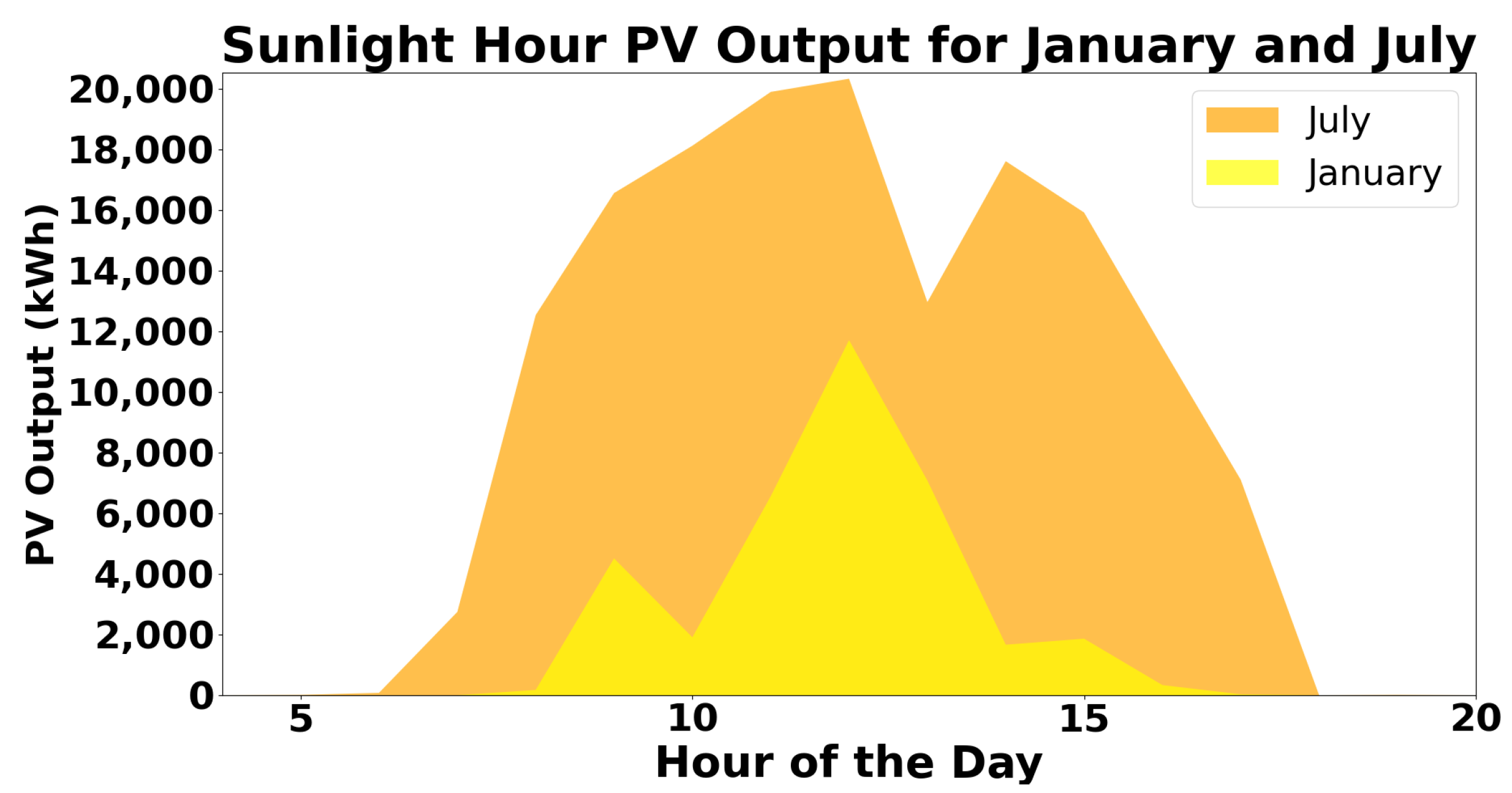
Figure 1. Twenty-four hours of June and July stochastically generated hourly PV outputs from fitted distributions of real-world PV units in Knoxville, TN.
Energies 17 02821 g001
Figure 2. Stochastically generated hourly demands from fitted distributions of real-world buildings.
Energies 17 02821 g002
Figure 3. Markov decision tree model of EMS. At time beginning of t 0 , an action A is taken, and with some probability P( Z m , t ) the PV energy output being high enough to meet demand alone (H), or too low (L) resulting in some cost at at the start of the next time step R t 1 ( A ) based on the action taken.
Energies 17 02821 g003
Figure 4. Average daily costs (returns) during training of the PPO-G. This plot visualizes the agent improving the EM policy during training.
Energies 17 02821 g004
Figure 5. Demand covered by EMS method in island mode.
Energies 17 02821 g005
Figure 6. Demand covered by EMS method during intermittent disruptions.
Energies 17 02821 g006
Figure 7. Energy dynamics over a 24 h period as modeled by the PPO-G show distinct patterns. When the orange demand bar exceeds others, it indicates times when demand surpassed supply, incurring a cost. Hours with a blue bar at the top, such as hours 0−2, signify periods when the ESS unit was discharged, supplying more than needed. When the green bar is at the top, the combined power from the ESS and PV units sufficiently meets energy demands. Hours where the yellow PV bar tops the green bar indicate times when the ESS is being charged by the PV unit, reducing the total energy supplied. In a grid-connected scenario, the EMS model allows the ESS to provide supplemental energy outside sunlight hours, charge during sunlight hours, mostly meet demands, and generate profits during peak PV output hours by supplying excess energy.
Energies 17 02821 g007
Figure 8. Energy dynamics for a 24 h period of EMS during an islanded scenario produced by A2C−D model. Green represents the summation of the DG output (ESS + PV), orange represents the level of demand at the indicated hours, blue indicates some ESS energy exchange either discharging (above origin) or charging (below origin). Areas where the orange bars are the top bars indicate hours where some number of energy demands went unmet. The proportion of orange above the blue ESS output and green total ESS and PV output bars represents the amount of supply lacking.
Energies 17 02821 g008
Table 1. Sets used for MG model and optimization.
SetsDescription
F set of facilities to be energized
G distributed generation unit { P , E }
A set of potential actions { discharge ( 0 ) , charge ( 1 ) , idle ( 2 ) }
C states representing ESS charge level {0 (empty), ..., N (full)}
M set of months the EMS policy will be evaluated
H time units representing the hour of a day { h 0 , . . . , h 23 }
Table 2. Variables used for MG model and optimization.
VariablesDescription
P m , h expected PV output at time h based and m
E h , a ESS output at time h based on action a
C h number of consecutive discharges with no charge at h
δ f , h demand for facility f over hour h
L h load demand by F over h
D M day of month M
S h power supply from G over h
T h difference between energy demanded and energy supply
R h cost or profit for energy bought/sold at time h
B h energy cost/burden at time h
Table 3. Parameters used for MG model and optimization.
ParameterDescription
κ peak demand energy price USD/kWh)
ϵ ESS nameplate power rating (kWh)
Δ maximum consecutive discharges ESS can provide from a full charge
ρ PV nameplate power rating (kW)
γ penalty for exceeding ϕ
Table 4. This table shows the average daily cost and demand coverage percentage for tested policy generation methods. G indicates trained while grid connected, while D indicates trained with monthly intermittent disruptions.
MethodCost CoverageDemand Coverage
RNG44%47%
Greedy59%53%
PPO-G86%61%
A2C-G83%62%
PPO-D69%53%
A2C-D51%52%
Disclaimer/Publisher’s Note: The statements, opinions and data contained in all publications are solely those of the individual author(s) and contributor(s) and not of MDPI and/or the editor(s). MDPI and/or the editor(s) disclaim responsibility for any injury to people or property resulting from any ideas, methods, instructions or products referred to in the content.