Abstract
At present, the condition assessment of transformer winding based on frequency response analysis (FRA) measurements demands skilled personnel. Despite many research efforts in the last decade, there is still no definitive methodology for the interpretation and condition assessment of transformer winding based on FRA results, and this is a major challenge for the industrial application of the FRA method. To overcome this challenge, this paper proposes a transformer condition assessment (TCA) algorithm, which is based on numerical indices, and a supervised machine learning technique to develop a method for the automatic interpretation of FRA results. For this purpose, random forest (RF) classifiers were developed for the first time to identify the condition of transformer winding and classify different faults in the transformer windings. Mainly, six common states of the transformer were classified in this research, i.e., healthy transformer, healthy transformer with saturated core, mechanically damaged winding, short-circuited winding, open-circuited winding, and repeatability issues. In this research, the data from 139 FRA measurements performed in more than 80 power transformers were used. The database belongs to the transformers having different ratings, sizes, designs, and manufacturers. The results reveal that the proposed TCA algorithm can effectively assess the transformer winding condition with up to 93% accuracy without much human intervention.
1. Introduction
Power systems depend heavily on transformers, which play a crucial role in the transmission and distribution of electric power. Although transformers are generally reliable pieces of equipment, the increasing power demand and continuous exposure of power transformers to various system faults result in elevated electrical and mechanical stresses that increase the likelihood of failures. Many failure mechanisms ultimately limit the useful operating life of the transformer. Anticipating different failure modes and taking pre-emptive measures are the key to extending the life of the transformer [1,2,3].
Accordingly, different condition assessments and diagnostic techniques have been developed to identify faults within power transformers [4]. Among these methods, frequency response analysis (FRA) is a non-intrusive and non-destructive diagnostic tool to identify a variety of faults in the transformer’s active part [5,6]. The FRA measurement process has been standardized through research in the past, as documented in IEC and IEEE standards [7,8]; however, there is still no globally accepted methodology for interpreting FRA results. Consequently, transformer condition assessment using the FRA method demands skilled personnel. Therefore, the interpretation of FRA has become a leading topic with different research bodies, i.e., IEEE, IEC, and CIGRE. Recently, CIGRE WG A2.53 drafted a technical brochure containing interpretation guidelines for FRA [9].
The numerical indices method is the most widely used approach for FRA interpretation [10,11]. These indices quantify changes between two FRA signatures, and the condition of the transformer, healthy/deformed, is decided based on the value of the index. Currently, indices are calculated in the fixed-frequency ranges. However, standards [7,8] state that the frequency sub-bands vary with the transformer size and rating, and no general range can be determined. Moreover, the threshold values of the indices to differentiate between the transformer’s healthy and faulted conditions are not defined yet. Due to the absence of an effective diagnosis procedure, all commercial FRA equipment computes numerical indices based on fixed-frequency sub-bands. Moreover, at this stage, fault classification is also not possible [9]. An effective assessment method should provide both features, i.e., identification of the condition of the transformer and classification of the fault type, so that necessary remedial measures can be initiated.
Artificial intelligence (AI) and machine learning techniques have been of great interest lately for transformer condition assessment and diagnosing faults [12,13,14]. However, in FRA, very few attempts have been made using such techniques. Velasquez et al. (2011) [15] employed a decision tree model to classify low-frequency and high-frequency faults. Data from 500 transformers were employed for time-based comparison. Bigdeli et al. (2012) [16] employed a support vector machine (SVM) model to discriminate between different mechanical fault types. In this work, only two types of transformers were employed, a classic 20 kV transformer and a model transformer. Ghanizadeh et al. (2014) [17] employed an artificial neural network (ANN) to identify electrical and mechanical faults with good accuracy. However, a single 1.2 MVA transformer model was employed in this research. Gandhi et al. (2014) [18] used nine statistical indices and 90 FRA cases to develop a three-layer ANN. The main disadvantage of this work is that only a single transformer model was employed to generate the database. Aljohani et al. (2016) [12] employed digital image processing to automate fault identification; however, only two transformers of different ratings were simulated for this purpose. Luo et al. (2017) [19] employed ANN to recognize simulative winding deformation faults to different extents. In this contribution, transfer function, zeros, and poles were considered to be the features of ANN; however, the faults were simulated only in a transformer simulation model. Liu et al. (2019) [20] used the SVM model to diagnose three different types of faults, i.e., disk space variation, radial deformation, and inter-turn fault. Numerical indices were employed to extract eight features from FRA data. An accuracy rate of 96.3% was obtained in this contribution. Zhao et al. (2019) [21] introduced a winding deformation fault detection method. The method is based on the analysis of binary images extracted from FRA traces to improve FRA interpretation. The digital image processing technique is used to process the binary image and the outcome of this method is a fault detection indicator. Duan et al. (2019) [22] proposed a deep learning algorithm to detect inter-turn faults in transformers with an accuracy of 99.34%. However, the feasibility of this classification algorithm was assessed only with simulated and preliminary experimental data. Mao et al. (2020) [14] proposed a support vector machine (SVM) model to identify the winding type, which is critically important from an asset management point of view. However, with the changes in the transformer rating, the dominated frequency region also changes, which makes it difficult to generalize this model.
The results of these reports show the potential of AI and machine learning algorithms for fault diagnosis and classification. However, the performance of some classifiers, e.g., decision trees, can be further improved by using ensembled machine learning models. Most of these studies employed small datasets. Additionally, fixed-frequency sub-bands are considered to calculate the numerical indices, whereas standards state that the ranges of frequency sub-bands cannot be fixed as they depend on transformer ratings. Moreover, only a few faults are classified and a small number of transformers are employed, which decreases the diversity of fault patterns. Hence, a diverse dataset of various faults from the field is necessary to settle the criteria for using AI and ML methods.
The innovative contributions of this paper, if compared to previous studies, are as follows:
- Mainly six common conditions of the transformers are identified which cover a variety of transformer faults, i.e., radial deformation, axial collapse, disk space variation, conductor tilting/twisting, short-circuited windings, open circuit, etc. Moreover, the effect of different oils, temperatures, and saturations on the core is also identified.
- Features are extracted using an adaptive frequency division algorithm. In previous studies, fixed-frequency sub-bands are considered to calculate the numerical indices, whereas standards state that the ranges of frequency sub-bands cannot be fixed as they depend on transformer ratings.
- A state-of-the-art transformer condition assessment (TCA) algorithm is proposed which is based on the numerical indices, as well as a supervised machine learning technique to develop a method for the automatic assessment of FRA measurements. Random forest (RF) classifiers were developed for the first time to identify the six common states/conditions of transformer windings.
- A comparison of the performance of different numerical indices to propose more suitable ones.
- The application of the TCA algorithm to a variety of real transformers, i.e., generator step-up unit, distribution, transmission, GIS connector, shunt reactor, dry type, etc., which are faulty during operation.
2. Random Forest Classification Model
A random forest (RF) algorithm is among the most effective algorithms for classification. RF classifiers are simple, fast, robust, and have proven to be successful in various fields [23]. RF classifiers fall under the umbrella of ensemble-based machine learning models, which use an ensemble of decision trees (DTs). DTs classify patterns using a sequence of well-defined rules. It is a tree-like classification algorithm, where attributes of the dataset are represented by internal nodes, decision rules are represented by branches, and the result of the cumulative decisions is represented by leaf nodes as shown in Figure 1. The leaf node contains cases belonging to a single class (pure node).
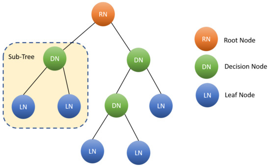
Figure 1.
Flow chart representation of decision tree.
In RF, several decision trees are trained by randomly chosen subsets of the dataset that has the same size as the original training set. A final class for the test object is then determined by combining the votes from the various decision trees. It supports the basic concept that a combination of weak learners can build a strong learner [24].
DTs are grown by splitting the data recursively. To determine the best features as splitters, mainly three measures are commonly used, i.e., Gini index (GI), information gain ratio (IGR), and information gain (IG). In this research, the C4.5 algorithm is employed, which is based on the information gain ratio [23].
Information Gain Ratio (IGR)
The information gain ratio (IGR) is used to identify the features that give maximum information about a class. IGR is derived from information gain, which measures entropy reduction at each split. If the proportion of samples of class k in dataset D containing C classes is , the information entropy of D is defined as follows:
An attribute that provides a maximum reduction in entropy is selected as a splitter at the current node. Suppose the attribute x with N possible outcomes is used to divide the set D, N nodes are generated, wherein the nth node contains all samples in D that take the value of on attribute x, denoted as . The expected entropy if x is used as the current root is measured as
The information gained by selecting x to partition data is
However, the information gain is biased toward the attribute with many distinct values. To overcome this problem, attributes that cause many splits are penalized. Hence, the extent of partitioning is calculated by Splitinfo. This normalizes the information gain, resulting in the calculation of the gain ratio.
Random forests improve predictive accuracy and control high variance and overfitting in decision trees [25]. During the training process, the bagging technique is used to generate several subsets of data. Individual trees are trained on these bootstrapped subsets. Each tree predicts a class and the class with majority voting is assigned to the observation. A random forest model with N decision trees is shown in Figure 2.
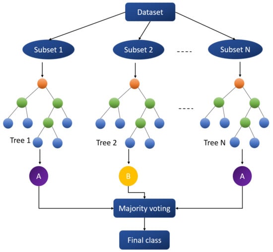
Figure 2.
Flow chart representation of random forest.
3. Methodology
The necessary steps to build the TCA algorithm for a given dataset are illustrated in Figure 3. The process involves six main steps, i.e., data preparation, generation of features, training of the classifier, testing of the classifier, validation of results with unseen data, analysis of performance, and validation of results with selected unseen cases. If the performance is not satisfactory, it can be mainly due to inaccurate data preparation, imprecise feature generation, or less diverse traces in different classes. In such cases, the TCA algorithm suggests redefining the process steps to improve performance.
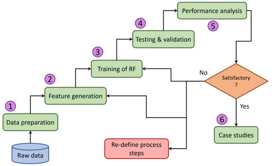
Figure 3.
Workflow for development of TCA algorithm.
3.1. Data Pre-Processing
Data pre-processing involves two steps: data labeling and noise removal. In this research, the data from 139 FRA measurements performed in more than 80 power transformers were used. The database was obtained from transformers having different ratings, sizes, designs, and different manufacturers. These cases were collected in collaboration with CIGRE WG A2.53 [9]. Additionally, the data of real case studies were collected from the field from different utilities and diagnosis companies, and FRA measurements where winding deformations were simulated in different transformers were also used [9]. The database consists of different types of transformers, i.e., transmission units, distribution units, generator step-up units, shunt reactors, GIS connectors, dry type, etc. In this paper, the data of open-circuit FRA measurements were employed for the development of the TCA algorithm. Moreover, reference data were also obtained for all the cases in the database. In the database, each FRA measurement belongs to a predefined state of the transformer. Six transformer conditions are identified which are healthy winding, healthy winding with core saturation, mechanical faults, shorted turns between conductors, open circuit, and repeatability issues. Each condition is labeled as a class (A to F). The distribution and description of classes in the database are presented in Figure 4 and Table 1, respectively.
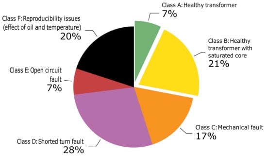
Figure 4.
Distribution of classes in the database.

Table 1.
Description of classes in the database.
Generally, the data provided may be partly accompanied by noise signals which can cause several small peaks and valleys at the lower frequencies. This noise was removed using a moving average Gaussian filter. An example of the FRA signature before and after denoising is shown in Figure 5.
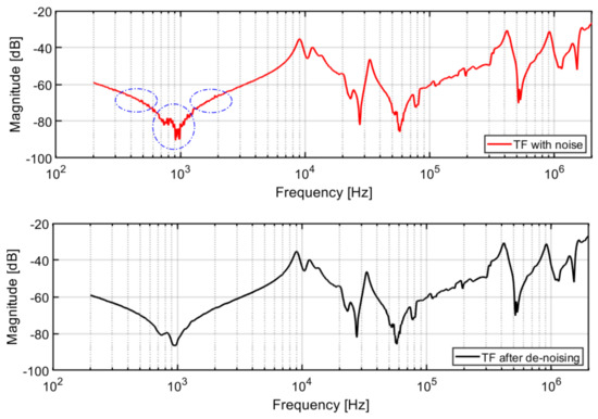
Figure 5.
Comparison of the FRA signature before (up) and after (down) denoising.
3.2. Feature Generation
Feature generation also involves two steps. Firstly, the entire frequency spectrum of the FRA is divided into four frequency sub-bands, i.e., two low-frequency sub-bands (LFB1 and LFB2), a medium-frequency sub-band (MFB), and a high-frequency sub-band (HFB). The adaptive frequency division algorithm is employed, which successfully identifies low-, medium-, and high-frequency regions in open-circuit FRA measurement depending upon transformer size, rating, winding type, and connection scheme. The details of the adaptive frequency division algorithm are described in the author’s previous work [26]. It is important to note that the presented frequency division structure is applicable to open-circuit FRA measurements.
Secondly, six numerical indices, i.e., LCC, CCF, SD, SDA CSD, and SE, were employed to quantify the changes between reference and current FRA signatures in each frequency sub-band. The detailed definition and equations can be found in the author’s previous work [10]. Thus, each index gives 4 features from a single FRA measurement which will serve as features for the TCA algorithm. An example of frequency sub-band division and feature generation from a typical FRA measurement is presented in Figure 6. After frequency division and feature generation, it is possible to generate deviation patterns for the given six conditions of the transformer as shown in Table 2. These patterns of deviations are based on the case studies in the database containing 139 FRA measurements from 80 power transformers. A similar kind of trend can be found in various case studies presented in the literature, especially in IEEE and IEC standards [7,8]. These deviation patterns will serve as a basis for the TCA algorithm.
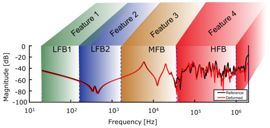
Figure 6.
Graphical representation of frequency sub-band division and feature generation in a typical FRA measurement.
Table 2.
Deviation patterns for different transformer conditions.
3.3. Training and Testing of Random Forest
In this step, RF was trained with 133 FRA measurements while 6 cases were reserved for case studies. The input provided is a feature matrix (133 × 4) and the label matrix (133 × 1). The label matrix is the class of each case, such as class A to F. The model learns from the training data and predicts the output (the class of the test data).
To ensure that every observation from the dataset appears in the train and test sets, the K-fold cross-validation technique was employed. K-fold cross-validation is a resampling procedure used to evaluate the ML model on a limited database. In this method, data are divided into K subsets (folds), then the model is trained using K-1 folds and tested on the Kth fold. This procedure is repeated K times so that every fold is tested once as illustrated in Figure 7. This procedure results in K different models fitted on different yet partly overlapping training sets and tested on non-overlapping test sets.
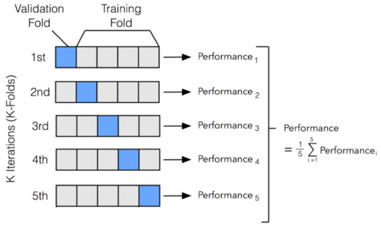
Figure 7.
Representation of 5-fold cross-validation technique.
Finally, the cross-validation performance was computed as the arithmetic means over the K performance estimates. The choice of K is arbitrary and there is a bias–variance tradeoff associated with it. Usually, 5 or 10 is an ideal choice [27]. Taking into account the small dataset, 5-fold stratified cross-validation was used in this research. StratifiedKfold ensures stratified folds, i.e., the percentage of samples from each of the target classes is roughly equal in each fold. This implies that during each iteration the model is trained with a feature matrix (106 × 4) and the label matrix (106 × 1), while it is tested with a feature matrix (27 × 4). This process is repeated five times. After five iterations, the arithmetic mean of the performance is computed. In this way, the model is tested on each set of data and the variance of results is reduced.
3.4. Performance Analysis
At this stage, the performance of the algorithm was evaluated via performance evaluation metrics. Mainly, five performance evaluation metrics, i.e., accuracy, precision, recall, F-score, and confusion matrix, were employed in this research, which provide the general and detailed (per class) performance of the algorithm. The performance evaluation metrics used in this work are described below:
where
- True Positive (TP): transformer is healthy (positive), and is predicted to be healthy (positive).
- False Negative (FN): transformer is healthy (positive), but is predicted to be faulty (negative).
- False Positive (FP): transformer is faulty (negative), but is predicted to be healthy (positive).
The predictive performance of the TCA algorithm trained with different numerical indices is summarized using confusion matrices as illustrated in Figure 8. The confusion matrices were obtained using the 5-fold cross-validation method in Python. The diagonal cells show the number of correctly classified cases for each class, while off-diagonal cells represent the number of misclassified cases. The classification performance of the TCA algorithm trained with different numerical indices is briefly described as follows:
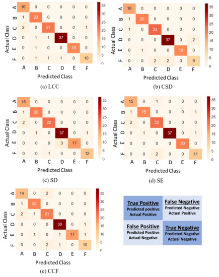
Figure 8.
Confusion matrices for 5-fold cross-validation of TCA algorithm trained with different indices: (a) LCC, (b) CSD, (c) SD, (d) SE, and (e) CCF.
TCA trained with LCC (Figure 8a): The performance of TCA for class A is excellent, as 100% of the cases are correctly identified. The performance for classes B and E is good, as only one case is misclassified in each class. The performance of class D is acceptable, as only two cases are misclassified. The performance of classes C and F is poor as three cases in each class are misclassified. The reason behind this is that the FRA traces of a slight mechanical change for a power transformer are similar to the FRA traces of a normal transformer.
TCA trained with CSD (Figure 8b): The performance of TCA for class A is excellent, as 100% of the cases are correctly classified. The performance of classes B, C, and E is good, as only one case in each class is misclassified. The performance of class D is acceptable, as only two cases are misclassified. However, the performance of class F is poor, as four cases are misclassified.
TCA trained with SD (Figure 8c): The performance of TCA for class A is excellent, as 100% of the cases are correctly classified. The performance of classes B and F is good, as only one case in each class is misclassified. The performance of classes C and D is acceptable, as only two cases are misclassified. However, the performance of class E is low, as three cases are misclassified as class D.
TCA trained with SE (Figure 8d): The performance of TCA for class E is excellent, as 100% of the cases are correctly identified. The performance of class A is good, as only one case is misclassified. The performance of classes B, C, D, and F is acceptable, as only two cases are misclassified in each class.
TCA trained with CCF (Figure 8e): The performance of classes B and D is good, as only one case is misclassified in each class. The performance of class A is acceptable, as only two cases are misclassified as class C. However, the performance of classes C, E, and F is poor, as three cases in each class are misclassified.
Error identification is performed using error analysis which helps to isolate, observe and diagnose erroneous predictions, thereby helping to understand pockets of high and low performance of the TCA algorithm. Table 3 summarizes the results of the error analysis in different classes. In Table 3, a list of possible hypotheses for error distribution is presented. Slight mechanical deformations are confused with slight deviations due to the influence of oil and temperature. Moreover, it can also be seen that some classes have the same dominant frequency range, such as shorted turn fault and core saturation. As both types affect the FRA trace in the low-frequency region, open-circuit/lose connection faults and short circuit faults also share the same dominant frequency range. It can be seen that CSD shows the best performance for detecting small mechanical deformations. Moreover, the CSD feature exhibits the lowest false-positive (predicted healthy, actually faulty) rate. However, it should be noted that the percentage error is highly dependent on an imbalanced class distribution.
Table 3.
Error analysis of TCA algorithm.
Under the premise of imbalanced class distribution, a classifier can exhibit good performance for specific classes (usually majority classes), which does not necessarily imply that the classification of all classes is good. For this purpose, precision, recall, and F1 score metrics (PRF) are used. Where precision is a measure of the correctness of a positive prediction, recall is the measure of how many true positives are predicted from all positives in the dataset, and F1 score is the harmonic mean of recall and precision. A comparison of PRF trained with different indices along with the number of instances is shown in Figure 9.
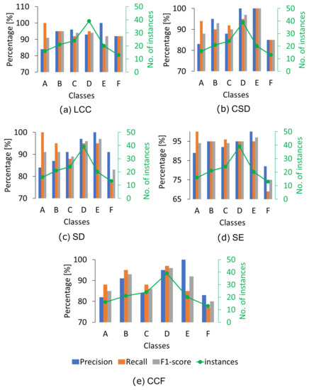
Figure 9.
Comparison of precision, recall, and F1 score of TCA algorithm trained for different indices: (a) LCC, (b) CSD, (c) SD, (d) SE, and (e) CCF.
TCA algorithm trained with LCC: Class A has the lowest precision, which means that class A has higher false positives (TCA predicts healthy winding but these were not healthy). Class F has lower recall, which means that class F has higher false negatives (TCA could not predict some cases to class F but these belonged to class F). However, the average F1 score for all classes is above 90%.
TCA algorithm trained with CSD: Precision, recall, and F1 score for all classes are above 90% except for class F, which has the lowest precision and recall, indicating class F has higher false positives and higher false negatives, respectively. However, the average F1 score for all classes is 91.6%.
TCA algorithm trained with SD: Class A has the lowest precision, indicating class A has higher false positives, while class E has lower recall, indicating class F has higher false negatives. However, the average F1 score for all classes is 93%.
TCA algorithm trained with the feature set SE: Class F has the lowest precision and recall, indicating class F has higher false positives and higher false negatives, respectively. However, the average F1 score for all classes is 92%.
TCA algorithm trained with SE: Classes A and F have the lowest precision and recall, indicating these classes have higher false positives and higher false negatives, respectively. However, the average F1 score for all classes is 88%, which is the lowest of the selected indices.
Figure 10 shows the comparison of the accuracy of the TCA algorithm for different numerical indices. It can be seen that TCA trained with CSD, SD, and SE shows the highest performance. The average overall accuracy for these three indices is 93%. The average overall accuracy for LCC is 92%. However, the accuracy of the TCA algorithm for CCF is relatively low, as only 90% of the cases are correctly identified. It can also be observed that the TCA algorithm trained with CCF feature sets has more misclassified cases than other numerical indices.
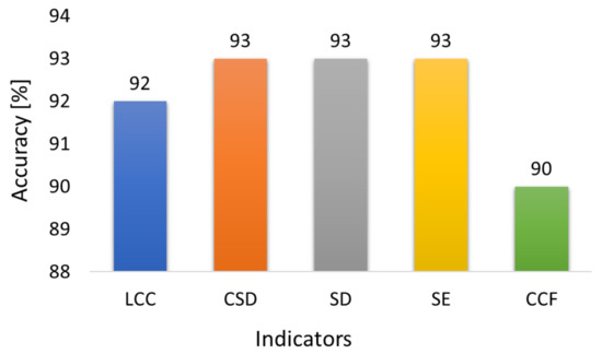
Figure 10.
Comparison of accuracy of TCA algorithm trained for different indices.
3.5. Case Studies
3.5.1. Case 1: Axial Collapse after Clamping Failure
In case 1, FRA measurements of a three-phase, 240 MVA, 400/132 kV autotransformer are considered [9]. After the Buchholz alarm, the transformer was switched out of service for further investigation. FRA open-circuit measurements were performed on common winding and the results were compared with the reference measurements as shown in Figure 11.
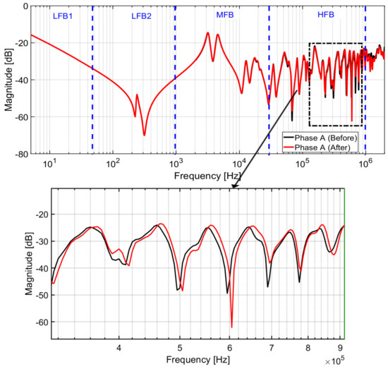
Figure 11.
LV winding open-circuit FRA before and after fault.
The visual analysis of the FRA measurements shows significant deviations and shifts in some resonances in the high-frequency region. After dismantling, it was found that A-phase LV winding was axially damaged and twisted as shown in Figure 12. The case was further tested with the TCA algorithm trained with different indicators. The performance metrics are shown in Table 4. It can be seen that TCA trained with different indicators has successfully diagnosed this case.
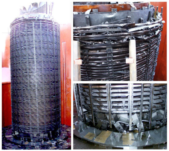
Figure 12.
Axial collapse of LV winding due to clamping failure [9].
Table 4.
Performance analysis of TCA for case 1.
3.5.2. Case 2: Open Circuit Fault
A three-phase, 34 MVA, 237/5.65 kV; the transformer was switched out of service for investigation. The HV winding open-circuit FRA measurements before and after the fault are shown in Figure 13 [9]. At low frequencies, an increase in the attenuation accompanied by a vertical shift downwards can be observed, which indicates that the open circuit does not completely break the electrical connection of the winding. At high frequencies, the peaks do not show frequency shifts, but the vertical shifts are a clear indication of the change in the resistance of the winding. After dismantling, it was confirmed to be an open-circuit fault. The case was further tested with the TCA algorithm and results are presented in Table 5. All indicators have predicted the correct fault class.
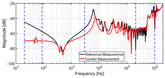
Figure 13.
FRA of HV winding before and after the fault.
Table 5.
Performance analysis of TCA for case 2.
4. Conclusions
This paper presents a transformer condition assessment algorithm for the automatic assessment of transformer FRA results. A combined approach of numerical indicators and a random forest machine learning classification model is used. The six most common states of transformer windings are considered in this research. The data from 139 FRA measurements performed in more than 80 power transformers were used. The classification capabilities of TCA trained with different indices are compared based on accuracy in the five-fold cross-validation method. It was found that the TCA algorithm exhibits good performance, as 90% of the cases were correctly identified by TCA trained with different indicators. However, provided with the feature sets of CSD, SD, and SE, the TCA algorithm shows excellent performance, as 93% of the cases were correctly classified, indicating the best numerical indices for the winding fault detection and classification using FRA measurements. The performance was also validated using selected case studies from real power transformers with known diagnoses and it was noticed that all cases were correctly classified by the TCA trained with different feature sets. However, the RF classification model is used with default parameters, and hyper-parameter tuning should also be tested on a comparatively larger database. The results obtained in this paper confirm that the proposed TCA algorithm can effectively assess the condition of transformer winding and also recognize the type of fault with good accuracy.
Author Contributions
M.T. developed the random forest algorithm, conceptualized the automatic frequency division technique, conducted the classification, and performance analysis, and composed the manuscript. S.T. acquired the funding, supervised the research, and edited the manuscript. All authors have read and agreed to the published version of the manuscript.
Funding
This research was funded by the Deutsche Forschungsgemein-schaft (DFG, German Research Foundation)—380135324.
Acknowledgments
The authors would like to thank all members of Cigré Working Group A2.53 for their valuable support for the collection of fault cases and preparation of the database. The authors also appreciate the discussions within Cigré Working Group A2.53 “Advances in the interpretation of transformer Frequency Response Analysis (FRA)”.
Conflicts of Interest
The authors declare no conflict of interest.
References
- Bagheri, S.; Moravej, Z.; Gharehpetian, G.B. Classification and Discrimination Among Winding Mechanical Defects, Internal and External Electrical Faults, and Inrush Current of Transformer. IEEE Trans. Ind. Inf. 2018, 14, 484–493. [Google Scholar] [CrossRef]
- Mortazavian, S.; Shabestary, M.M.; Mohamed, Y.A.-R.I.; Gharehpetian, G.B. Experimental Studies on Monitoring and Metering of Radial Deformations on Transformer HV Winding Using Image Processing and UWB Transceivers. IEEE Trans. Ind. Inf. 2015, 11, 1334–1345. [Google Scholar] [CrossRef]
- CIGRE WG A2.37; Transformer Reliability Survey. CIGRE Technical Brochure 642. International Council on Large Electric Systems: Paris, France, 2015.
- Tenbohlen, S.; Coenen, S.; Djamali, M.; Müller, A.; Samimi, M.; Siegel, M. Diagnostic Measurements for Power Transformers. Energies 2016, 9, 347. [Google Scholar] [CrossRef]
- Rahimpour, E.; Gorzin, D. A new method for comparing the transfer function of transformers in order to detect the location and amount of winding faults. Electr. Eng. 2006, 88, 411–416. [Google Scholar] [CrossRef]
- Jayasinghe, J.A.S.B.; Wang, Z.d.; Jarman, P.N.; Darwin, A.W. Winding movement in power transformers: A comparison of FRA measurement connection methods. IEEE Trans. Dielectr. Electr. Insul. 2006, 13, 1342–1349. [Google Scholar] [CrossRef]
- IEEE Std. C57.149-2012; IEEE Guide for the Application and Interpretation of Frequency Response Analysis for Oil-Immersed Transformers. IEEE Standard Association: New York, NY, USA, 2013.
- IEC60076-18; Measurement of Frequency Response, 1st Edition. International Electrotechnical Commission: Geneva, Switzerland, March 2012.
- CIGRE WG A2.53; Advances in the Interpretation of Transformer Frequency Response Analysis (FRA). CIGRE Technical Brochure 812. International Council on Large Electric Systems: Paris, France, 2020.
- Tahir, M.; Tenbohlen, S.; Miyazaki, S. Analysis of Statistical Methods for Assessment of Power Transformer Frequency Response Measurements. IEEE Trans. Power Deliv. 2021, 36, 618–626. [Google Scholar] [CrossRef]
- Tarimoradi, H.; Gharehpetian, G.B. Novel Calculation Method of Indices to Improve Classification of Transformer Winding Fault Type, Location, and Extent. IEEE Trans. Ind. Inf. 2017, 13, 1531–1540. [Google Scholar] [CrossRef]
- Aljohani, O. Application of Digital Image Processing to Detect Short-Circuit Turns in Power Transformers Using Frequency Response Analysis. IEEE Trans. Ind. Inform. 2016, 12, 12. [Google Scholar] [CrossRef]
- Aljohani, O.; Abu-Siada, A. Application of DIP to Detect Power Transformers Axial Displacement and Disk Space Variation Using FRA Polar Plot Signature. IEEE Trans. Ind. Inf. 2017, 13, 1794–1805. [Google Scholar] [CrossRef]
- Mao, X.; Wang, Z.; Jarman, P.; Fieldsend-Roxborough, A. Winding Type Recognition through Supervised Machine Learning using Frequency Response Analysis (FRA) Data. In Proceedings of the 2019 2nd International Conference on—Electrical Materials and Power Equipment (ICEMPE), Guangzhou, China, 7–10 April 2019; pp. 588–591. [Google Scholar]
- Contreras, J.L.V.; Sanz-Bobi, M.A.; Banaszak, S.; Koch, M. Application of Machine Learning Techniques for Automatic Assessment of FRA Measurements. In Proceedings of the XVII International Symposium on High Voltage Engineering, Hannover, Germany, 22–26 August 2011; p. 6. [Google Scholar]
- Bigdeli, M.; Vakilian, M.; Rahimpour, E. Transformer winding faults classification based on transfer function analysis by support vector machine. IET Electr. Power Appl. 2012, 6, 268. [Google Scholar] [CrossRef]
- Ghanizadeh, A.J.; Gharehpetian, G.B. ANN and cross-correlation based features for discrimination between electrical and mechanical defects and their localization in transformer winding. IEEE Trans. Dielectr. Electr. Insul. 2014, 21, 2374–2382. [Google Scholar] [CrossRef]
- Gandhi, K.R.; Badgujar, K.P. Artificial neural network based identification of deviation in frequency response of power transformer windings. In Proceedings of the 2014 Annual International Conference on Emerging Research Areas: Magnetics, Machines and Drives (AICERA/iCMMD), Kottayam, India, 24–26 July 2014; pp. 1–8. [Google Scholar]
- Luo, Y.; Ye, J.; Gao, J.; Chen, G.; Wang, G.; Liu, L.; Li, B. Recognition technology of winding deformation based on principal components of transfer function characteristics and artificial neural network. IEEE Trans. Dielectr. Electr. Insul. 2017, 24, 3922–3932. [Google Scholar] [CrossRef]
- Liu, J.; Zhao, Z.; Tang, C.; Yao, C.; Li, C.; Islam, S. Classifying transformer winding deformation fault types and degrees using FRA based on support vector machine. IEEE Access 2019, 7, 112494–112504. [Google Scholar] [CrossRef]
- Zhao, Z.; Yao, C.; Tang, C.; Li, C.; Yan, F.; Islam, S. Diagnosing Transformer Winding Deformation Faults Based on the Analysis of Binary Image Obtained From FRA Signature. IEEE Access 2019, 7, 40463–40474. [Google Scholar] [CrossRef]
- Duan, L.; Hu, J.; Zhao, G.; Chen, K.; Wang, S.X.; He, J. Method of inter-turn fault detection for next-generation smart transformers based on deep learning algorithm. High Volt. 2019, 4, 282–291. [Google Scholar] [CrossRef]
- Rokach, L.; Maimon, O. Data Mining with Decision Trees: Theory and Applications, 2nd ed.; World Scientific: Hackensack, NJ, USA, 2015. [Google Scholar]
- Alppaydin, E. “Decision Trees” in Introduction to Machine Learning, 2nd ed.; MIT Press: Cambridge, MA, USA, 2020; pp. 185–206. Available online: https://mitpress.mit.edu/books/introduction-machine-learning (accessed on 30 January 2023).
- Pedregosa, F.; Varoquaux, G.; Gramfort, A.; Michel, V.; Thirion, B.; Grisel, O.; Blondel, M.; Prettenhofer, P.; Weiss, R.; Dubourg, V.; et al. Scikit-learn: Machine learning in Python. J. Mach. Learn. Res. 2011, 12, 2825–2830. [Google Scholar]
- Tahir, M.; Tenbohlen, S. Transformer Winding Condition Assessment Using Feedforward Artificial Neural Network and Frequency Response Measurements. Energies 2021, 14, 3227. [Google Scholar] [CrossRef]
- Apt, K.R. Principles of Constraint Programming; Cambridge University Press: Cambridge, MA, USA; New York, NY, USA, 2003. [Google Scholar]
Disclaimer/Publisher’s Note: The statements, opinions and data contained in all publications are solely those of the individual author(s) and contributor(s) and not of MDPI and/or the editor(s). MDPI and/or the editor(s) disclaim responsibility for any injury to people or property resulting from any ideas, methods, instructions or products referred to in the content. |
© 2023 by the authors. Licensee MDPI, Basel, Switzerland. This article is an open access article distributed under the terms and conditions of the Creative Commons Attribution (CC BY) license (https://creativecommons.org/licenses/by/4.0/).