Best Practice Data Sharing Guidelines for Wind Turbine Fault Detection Model Evaluation

Abstract

In this paper, a set of best practice data sharing guidelines for wind turbine fault detection model evaluation is developed, which can help practitioners overcome the main challenges of digitalisation. Digitalisation is one of the key drivers for reducing costs and risks over the whole wind energy project life cycle. One of the largest challenges in successfully implementing digitalisation is the lack of data sharing and collaboration between organisations in the sector. In order to overcome this challenge, a new collaboration framework called WeDoWind was developed in recent work. The main innovation of this framework is the way it creates tangible incentives to motivate and empower different types of people from all over the world to share data and knowledge in practice. In this present paper, the challenges related to comparing and evaluating different SCADA-data-based wind turbine fault detection models are investigated by carrying out a new case study, the “WinJi Gearbox Fault Detection Challenge”, based on the WeDoWind framework. A total of six new solutions were submitted to the challenge, and a comparison and evaluation of the results show that, in general, some of the approaches (Particle Swarm Optimisation algorithm for constructing health indicators, performance monitoring using Deep Neural Networks, Combined Ward Hierarchical Clustering and Novelty Detection with Local Outlier Factor and Time-to-failure prediction using Random Forest Regression) appear to exhibit high potential to reach the goals of the Challenge. However, there are a number of concrete things that would have to have been done by the Challenge providers and the Challenge moderators in order to ensure success. This includes enabling access to more details of the different failure types, access to multiple data sets from more wind turbines experiencing gearbox failure, provision of a model or rule relating fault detection times or a remaining useful lifetime to the estimated costs for repairs, replacements and inspections, provision of a clear strategy for training and test periods in advance, as well as provision of a pre-defined template or requirements for the results. These learning outcomes are used directly to define a set of best practice data sharing guidelines for wind turbine fault detection model evaluation. The guidelines can be used by researchers in the sector in order to improve model evaluation and data sharing in the future.

1. Introduction

1.1. Motivation

The digital era offers many opportunities to the wind energy industry and research community. Digitalisation, defined as “the organisational and industry-wide use of data and digital technologies to improve efficiency, create insights, and develop products and services” [1], is one of the key drivers for reducing costs and risks over the whole wind energy project life cycle (https://windeurope.org/intelligence-platform/product/wind-energy-digitalisation-towards-2030/; accessed on 3 August 2022). The main opportunities relate to new processes and business models brought about by the availability—and innovative usage—of large amounts of data at all phases of the wind project life cycle. These can include, for example, digital twins, predictive maintenance, drones and expert systems, which can all contribute to reducing maintenance costs, increasing the amount of energy delivered as well as increasing efficiency.

However, the successful exploitation of these opportunities raises a number of challenges, which were recently thoroughly examined in [1]. This resulted in the definition of three “Grand Challenges” of wind energy digitalisation: (1) Creating findable, accessible, interoperable and reusable (FAIR) data frameworks [2]; (2) Connecting people and data to foster innovation; (3) Enabling collaboration and competition between organisations.

Solutions to overcoming these Grand Challenges have already been investigated to some extent, as described in [3]. Efforts include the Sharewind metadata registry [4], the IEA Wind Task 43 Metadata Challenge [5], digital platforms for collecting data from interactions with stakeholders [6], data marketplaces such as the IntelStor Market Intelligence Ecosystem (https://www.intelstor.com/; accessed on 3 August 2022), the EDP Open Data Platform (https://opendata.edp.com/; accessed on 3 August 2022), open-source tools including the Brightdata app (https://www.brightwindanalysis.com/brightdata/; accessed on 3 August 2022), OpenOA (https://github.com/NREL/OpenOA; accessed on 3 August 2022) and the Data Science for Wind Energy R Library (https://github.com/TAMU-AML/DSWE-Package/; accessed on 3 August 2022), as well as collaborative innovation processes [6,7]. However, none of these initiatives overcome the three Grand Challenges in a holistic manner, nor do they specifically enable cooperation between organisations or connect people and data.

In order to close this gap, a new collaboration framework called WeDoWind was developed in recent work by the present lead author [3], as summarised below. The main innovation of this framework is the way it creates tangible incentives to motivate and empower different types of people from all over the world to share data and knowledge in practice.

1.2. Literature Review

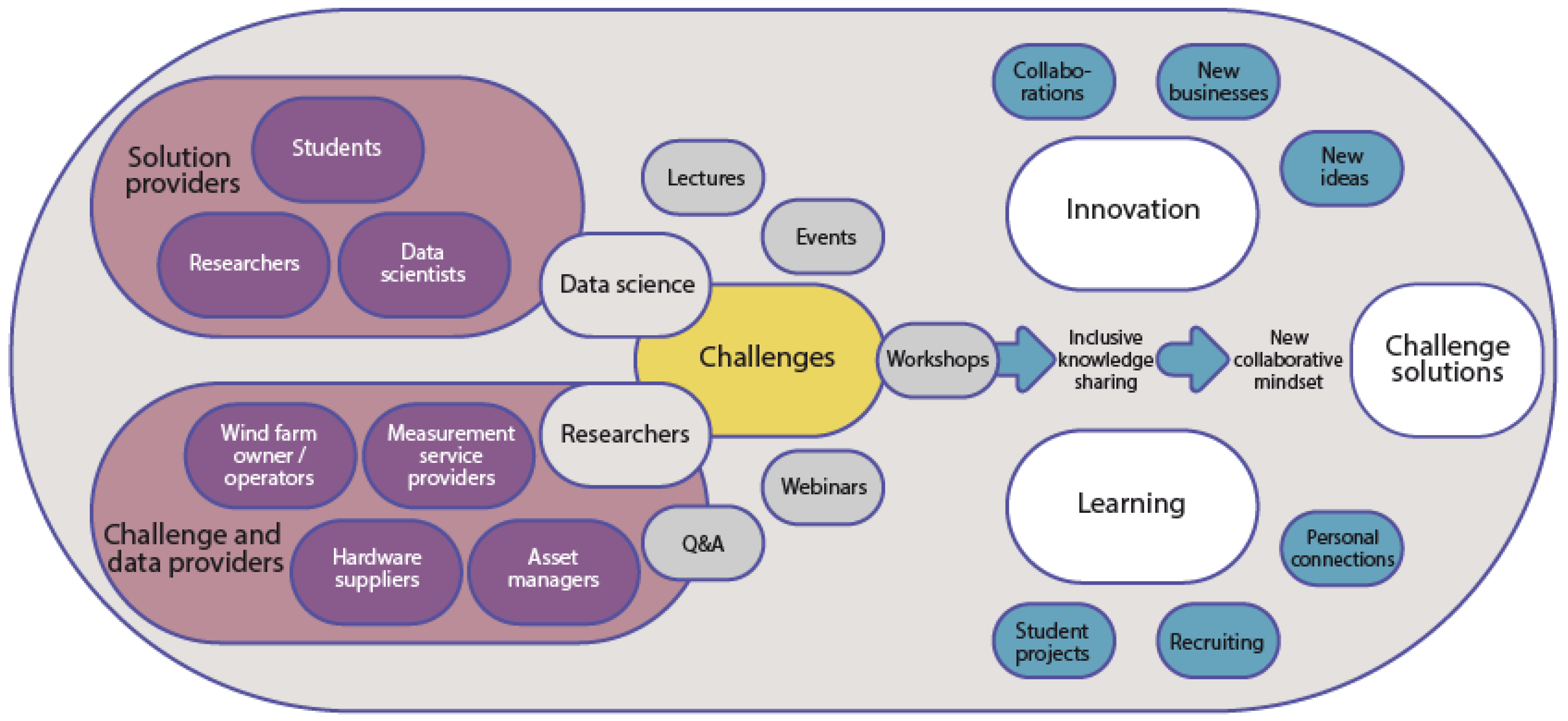
1.2.1. The WeDoWind Framework

The idea behind the WeDoWind framework is summarised in the value creation process in Figure 1. It brings together WeDoWind Challenge Providers, such as wind farm owner/operators, measurement service providers, hardware suppliers and asset managers, who provide data and WeDoWind Challenges, with Solution Developers, such as researchers, students and data scientists, who use the provided data to solve the WeDoWind Challenges. The data required in order to solve a particular WeDoWind Challenge are provided by the WeDoWind Challenge Providers under the confidentiality conditions they specify. This can include only allowing specific people to access their space, requiring them to sign agreements or preparing the data so that it is anonymous or normalised. A WeDoWind Challenge is defined as a fixed problem with a motivation, goal, expected outcome and deadline.

The WeDoWind Challenge Providers are motivated to participate because they receive diverse state-of-the-art solutions to their WeDoWind Challenges from international teams, increased visibility and contact with the research community. The Solution Developers benefit by getting access to relevant WeDoWind Challenges and data from the industry and getting visibility within a vibrant international research and teaching community. The digital platform allows all the data, code, meeting documentation, questions and discussions to be documented in one central location, meaning that it can be built upon in future WeDoWind Challenges and easily accessed by a wide range of people all over the world. The resulting community of active and passive challenge participants from academia and industry interested in sharing data, code and learning from each other forms a thriving and open digital wind energy ecosystem.

Ultimately, the framework allows the industry to adopt new approaches developed by academia much faster than is currently being done. This is because it allows the accumulation of data sets from multiple data providers in a unified format, providing a more realistic environment for developing and benchmarking new models. Additionally, it enables testing on how well the developed models scale to a large database, an integral requirement in practice. Finally, it can enforce transparency and robustness requirements for challenge solutions.

The case study demonstrated that the WeDoWind framework presents a promising solution for enhancing collaboration and data sharing in wind energy. It provided a number of benefits for both WeDoWind Challenge and Solution Providers, including access to data, code, knowledge and people skills. It was found to have high potential for use by the wider community, both within and beyond wind energy, by providing realistic environments for developing and benchmarking new machine learning (ML) models.

Furthmore, it allowed several challenges relating to the evaluation and comparison of different models to be identified. For example, the wide range of comparison metrics and Key Performance Indicators (KPIs) make it difficult to assess which metric or KPI is most suitable for a given application, especially when the heterogeneity of the models is high. As well as this, the conversion of these metrics into financial gains involves a number of different assumptions, and varying these assumptions in the EDP Challenge leads to a large variation in the results [3]. Finally, the quality of the evaluation results was thought to be dependent on the quality and quantity of provided data. These issues all require further investigation if data sharing and collaboration are to be improved in the sector.

In order to do this, multiple different WeDoWind Challenges need to be introduced and run, enabling both the accumulation of data sets from multiple data providers as well as the creation of an active community of people learning and sharing with each other. This effort is furthered in the current paper, with a focus on wind turbine fault detection based on SCADA (Supervisory control and data acquisition) data.

1.2.2. Wind Turbine Fault Detection Based on SCADA Data

The topic of wind turbine fault detection based on SCADA data is chosen for this work because it is an accessible topic for the industry and an interesting research topic for academia. SCADA data are more readily available than higher frequency data sets, and additional measurement equipment such as high-frequency Condition Monitoring Systems are not required.

Although the usage of SCADA data for wind turbine monitoring are attractive, its application is limited by the low resolution of the data (usually ten-minute averages). Therefore, fault detection methods based on SCADA data usually target secondary effects of the fault. Temperature monitoring is well-suited for detecting malfunctions in the components along the drive train, which account for the majority of turbine downtime [8]. Ref. [9] was among the first to apply the approach in the wind domain and prove its feasibility. Many publications with successful early detection of malfunctions followed, e.g., [10,11,12,13,14,15].

A recent review of the application of machine learning (ML) models for condition monitoring in wind energy shows that most models use SCADA or simulated data, and almost two-thirds of the methods use classification, the rest relying on regression. Neural networks, support vector machines and decision trees are most commonly used [16]. A wide range of ML methods have proven to be able to detect developing malfunctions at an early stage, often months before they resulted in costly component failures (see, e.g., [9,13,14,17]).

Furthermore, feature selection—a process of selecting variables that are significantly related to the outcome that the model is predicting—can be used to improve the success of condition monitoring based on SCADA data. For example, ref. [18] used deep learning to select the relevant variables related to transmission bearing temperature before analysing SCADA data. As well as this, ref. [19] propose an adaptive neuro fuzzy inference system to estimate the remaining useful life (RUL) of bearings based on vibration data and feature extraction. Other methods for predicting the RUL of wind turbine components include a feature fusion model based health indicator construction and self-constraint state-space estimator for bearings [20] and a novel health indicator for intelligent prediction of rolling bearing remaining useful life based on unsupervised learning model [21].

In the recent EDP Challenge mentioned in Section 1.2.1 above, the most promising models were found to be a Combined Ward Hierarchical Clustering and Novelty Detection with Local Outlier Factor (WHC-LOF) and a Combined Local Minimum Spanning Tree and Cumulative Sum of Multivariate Time Series Data (LoMST-CUSUM). The WHC-LOF solution combines the Ward Hierarchical Clustering [22], which identifies and removes anomalous clusters, with the Novelty Detection with Local Outlier Factor (LOF) [23], which is used to detect the outliers associated with the failures of the wind turbine. The LoMST-CUSUM solutions works in three stages as described in [24]. First, it establishes a so-called Minimum Spanning Tree (MST) using all data points. Second, it isolates the cluster anomalies by removing the links of the global MST one by one. Third, it repeats the second step to identify point-wise anomalies. At the end, an outlier score is assigned to each of the data points, indicating the anomaly level of the point. Cumulative sum (CUSUM) is a memory-type control chart that works by accumulating consecutive sample points over time to monitor changes in the process. CUSUM-based approaches have been used in wind turbine monitoring in combination with ML plots [25,26].

In addition to machine learning methods, Bayesian methods have shown advantages for statistical modelling and data analysis of uncertain and variable quantities, such as wind resource estimation, short-term forecasts [27] and fault detection. They are particularly useful time-varying or uncertain feature extraction. For example, a Bayesian and Adaptive Kalman Augmented Lagrangian Algorithm has recently been applied to wind turbine blade bearing fault detection [28] and a Probabilistic Bayesian Parallel deep learning framework as been applied to wind turbine bearing fault diagnosis [29].

Despite this progress, no particular model has yet been established as being optimal for SCADA-data-based fault detection. Furthermore, no comparison of the type, length and quality of data used in previous studies has been carried out systematically. Finally, the optimal comparison metric or KPI is not clear due to the high heterogeneity of models. However, various recent studies have concluded that more data should be made available and comparisons with a wide range of different data should be carried out in order to do this, e.g., [3,30,31]. We aim to contribute to this gap in the present work.

1.3. Contribution and Paper Organisation

In this paper, a set of best practice data sharing guidelines for wind turbine fault detection model evaluation are developed, which can help practitioners overcome the main challenges of digitalisation in wind energy, and are transferable to other industries that use data to create value.

The goals of this work are to (1) investigate the challenges related to comparing and evaluating different SCADA-data-based wind turbine fault detection models, and (2) to develop a set of best practice data sharing guidelines to improve model evaluation in the future. This aims to improve data sharing in the sector and therefore to address one of the largest barriers to implementing digitalisation. As the digital era progresses, data sharing and model evaluation are both going to grow, and therefore a thorough understanding of how to effectively perform these tasks is becoming increasingly important.

In order to achieve these goals, a new case study, the “WinJi Gearbox Fault Detection Challenge”, was carried out based on the WeDoWind framework. The case study is introduced in Section 2 and the submitted solutions are described and evaluated in Section 3. This includes a discussion of the difficulties related to comparing and evaluating the models at the end of the section. After that, in Section 4, a new set of best practice data sharing guidelines for wind turbine fault detection model evaluation are introduced, the WeDoWind framework is evaluated and discussed, and an outlook for its future transferability to other sectors is given. Finally, the conclusions are drawn in Section 5.

2. Case Study Description

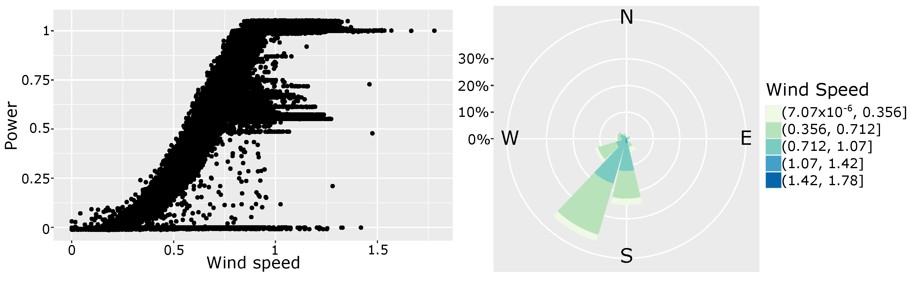
2.1. The Winji Gearbox Fault Detection Challenge

The WinJi Gearbox Fault Detection Challenge was provided by the Swiss asset management software provider WinJi AG, as described below:

We are an asset management software provider for renewable portfolios, also active in predictive maintenance. We have developed several methods for early prediction of faults based on SCADA data from wind turbines, achieving horizons of several days. Our aim is to push the performance of such predictions to at least a monthly horizon. Participants should make use of the provided SCADA data in order to train, test and validate methods that will provide clear indicators of an upcoming gearbox related fault, as well as/or a horizon-based probability of the event occurring. Over two years of 10-minute SCADA are provided, for five wind turbines in the same site. Two of these turbines experience gearbox failures leading to extended downtimes and one experiences bearing issues with no downtimes. The other two are free of significant failures. The dataset includes environmental, production and condition parameters as well as error information.

The data was anonymised by WinJi in the following ways:

• The power of each wind turbine was normalised by the rated power.
• The location and type of wind turbines was not provided.
• The time stamps were all shifted by an unspecified amount of time.
• The detailed fault information was not provided. Instead, fault occurrence indicators were provided as binary indicators, i.e., fault or no fault.

Whilst WinJi were involved strongly in the webinars in order to help and support the participants, they did not take part in the challenge themselves. This meant that a direct comparison between WinJi’s own analysis method and the new methods developed herein could not be carried out. WinJi was looking to learn from the challenge in order to further their knowledge indirectly. Their current method is based on a Normal Behaviour Model and is described further in [32].

Figure 2 shows the empirical power curve and wind rose (without filtering) for one of the wind turbines at the site (WT115). It can be observed that the power curve includes different operation conditions and the main wind direction is SSW.

2.2. The WeDoWind Framework

The WeDoWind framework was applied to the case study as follows:

• A dedicated space called “WinJi Challenges” was created on the digital platform together with WinJi. The WeDoWind Challenge description, including direct links to download the data, was developed together with WinJi and posted inside this space.
• A public “call for participants” website was created with a direct link to the registration form (https://www.wedowind.ch/spaces/winji-challenges-space; accessed on 5 April 2023). This was shared within the wind energy community using social media.
• A process for allowing WinJi to decide who may participate or not was set up. This process was not intended to reduce accessibility to the WeDoWind Challenge, but instead to ensure that applicants were real people interested in the WeDoWind Challenge and not robots, bots or imposters.
• A “Getting Started Guide” to using the digital platform was created and explainer videos were recorded in order to help users interact on the platform.
• A series of online workshops were organised for the participants—a launch workshop, interim workshops every month and then a final workshop. These involved brainstorming sessions in small groups as well as question and answer sessions with WinJi. The sessions were documented on a digital whiteboard and recordings were posted in the digital space.
• Regular email updates were sent with specific questions and actions to encourage interaction. This included requests to summarise and comment on different possible methods, as well as discussions of evaluation methods.
• The space was regularly checked, cleaned and coordinated by the WeDoWind developers to ensure that the information was up-to-date and understandable.
• Regular updates were communicated on social media during the challenge.

3. Submitted Solutions

3.1. Description of Submitted Solutions

A total of six solutions were submitted for the challenge. All of the solutions are summarised in

Table 1. Summary of all the submitted solutions.

Solution	Method	Contributor	Type	Goal	Pre-Proc.	Time Res.	Training Period
CAE-PSO	CAE	TUD	Unsup. Learn.	Pred. RUL	N (0, 1) Norm.	Minutes	100%
PM-DNN	DNN	ZSW	Sup. Learn.	Pred. Power Anomaly	N (0, 1) Norm.	Minutes	80%–20% random Blocks
DEC-DNN	DNN	ZSW	Sup. Learn.	Pred. Error Code	N (0, 1) Norm.	Minutes	80%–20% random Blocks
T-SNE	T-SNE	ZSW	Unsup. Learn.	Cluster Correlation	N (0, 1) Norm.	Minutes	80%–20% random Blocks
WHC-LOF	LOF	FISC	Unsup. Learn.	Pred. Anom. + RUL	WHC	Weeks	100%
TTF-RFR	RFR	MU	Sup. Learn.	TTF inference	Remove correlated features, stop instants	Hours	Leave one out (80%–20%)

and described in the next sub-sections below. The results are then presented in Section 3.2 and evaluated in Section 3.3. The contributors are TU Delft (TUD), the Center for Solar Energy and Hydrogen Research (ZSW), the Federal Institute of Santa Catarina (FISC) and Mondragon University (MU).

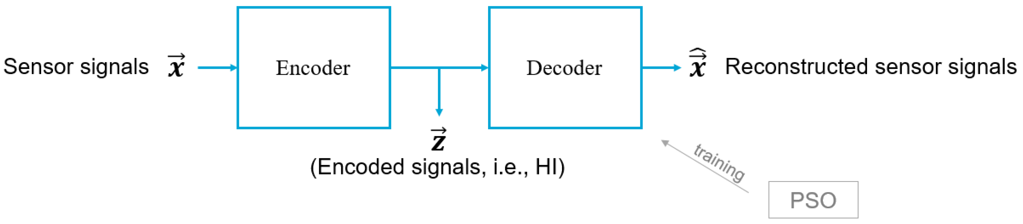
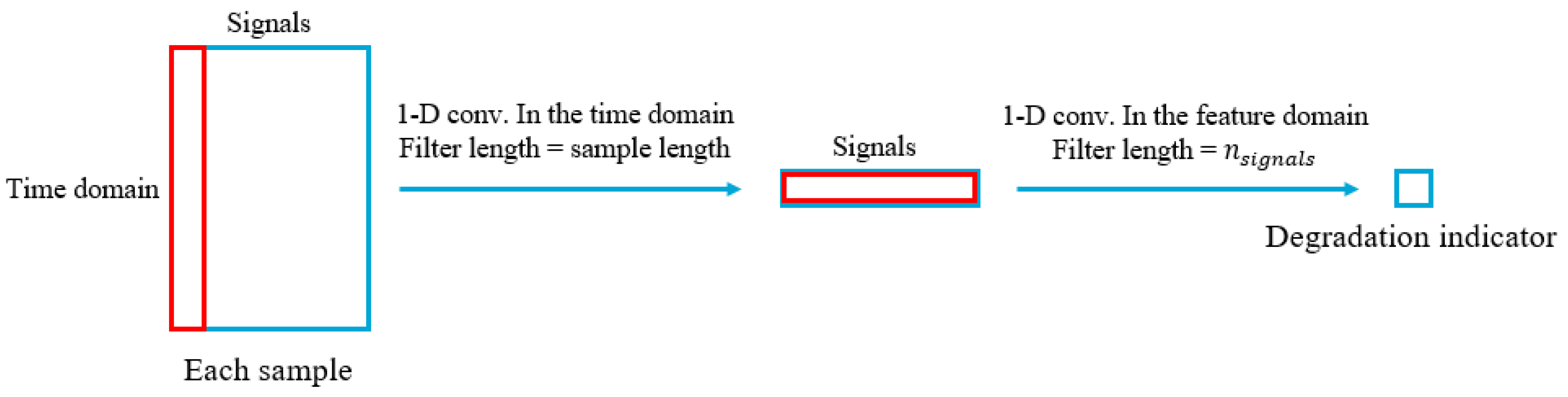
3.1.1. A Convolutional Autoencoder Trained with Particle Swarm Optimisation Algorithm for Constructing Health Indicators (CAE-PSO)

One of the most prevalent approaches for RUL estimation is constructing health indicators (HI), which are correlated with and act as proxies for the degradation process in the component studied. In this solution, a Convolutional Autoencoder (CAE) is proposed for unsupervised construction of health indicators from wind turbine SCADA data. The training cost function of the CAE is $f=|{\tau }_{\mathrm{MK}}|-MSE$, where $|{\tau }_{\mathrm{MK}}|\in [0,1]$ is the absolute value of the Mann–Kendall monotonicity score [33] of the HI constructed in the middle layer of the CAE and $MSE$ is the Mean Squared Error between the input signals and the reconstructed signals in the output layer (Figure 3). The training of the CAE is done by Particle Swarm Optimization (PSO) algorithm [34], which optimises the training cost function by searching the space of CAE weight parameters. The reason for using PSO rather than backpropagation for training the CAE is the fact that monotonicity is a metric related to the entire training set as a whole and not single samples or batches of samples from the training set which the network is trained on at each iteration of the backpropagation algorithm. Numerous algorithms have been proposed in the literature for both training Neural Networks and setting their hyperparameters, including evolutionary-based, swarm-based, and Bayesian-based [35,36,37]. However, PSO has been the most successful algorithm alternative to backpropagation for training Neural Networks [38]. By maximising the monotonicity of the constructed HIs, we aim at training the CAE to extract and isolate—from the SCADA signals—the factor that is related to the degradation of the component from other factors related to the operational and environmental conditions, process noise, etc. This is according to the fact that degradation is an irreversible and monotonic process. The proposed CAE is made up of an Encoder with two Convolutional layers. The first one performs convolution only in the time domain and the second one only in the feature domain. The Decoder is symmetric to the Encoder, as shown in Figure 4.

3.1.2. Performance Monitoring Using Deep Neural Networks (PM-DNN)

This was the primary approach of ZSW, and was chosen due to their positive experience with the method in many areas of renewable energy, including wind power for the early detection of icing. In this solution, the standard performance monitoring approach was investigated, using pure dense feed forward neural networks in the form of deep Multi-Layer Perceptron (MLP) [39] (otherwise known as Deep Neural Network (DNN)) trained with ADAM [40]. The used code is written in PyTorch [41]. The input data were normalised to a standard normal distribution (N(0, 1) Norm.). Since a validation set needs to be (I) from the same distribution as the training set, but (II) also be independent of the training set, the data were split into 200 blocks and 20% of the blocks were chosen randomly as validation data. This procedure is necessary, since the data are a time series and therefore shows high correlation from data point to data point. Pure random selection for the validation set would violate the rule for an independent validation set.

The DNN was trained with the wind turbine power output as a target. The hyper-parameters of the DNN architecture and the ADAM optimiser were optimised for the given data with Reinforcement Learning (RL). The validation set Mean Squared Error (MSE) was used as reward signal for the RL-Method Policy Gradients with Paramater-based Exploration (PGPE) [42]—we used the super symmetric, ranked version of the algorithm [43,44]. The PGPE implementation is an internal python/numpy code.

For the input data we ignored the error code itself, for obvious reasons. We assumed a Gaussian error distribution of the DNN and trained another DNN on the absolute differences of the prediction of the first DNN as a confidence model for the performance monitoring approach.

3.1.3. Direct Error Code Prediction Using DNNs (DEC-DNN)

This was the second approach of ZSW. It was applied because they wanted to know whether the error codes could be derived directly from the SCADA data and whether an increase in the probability of an error code could be observed in advance. For this, the same kind of DNN as in the PM-DNN solution was also used to investigated the naive approach, by training directly on the error codes as binary targets. The model was therefore a standard DNN with a logistic output activation function trained with ADAM and meta-optimised with PGPE. As an approximation, the output was interpreted as the probability of the occurrence of an error code.

The input data were again normalised to a standard normal distribution and split into validation and training sets by randomly choosing blocks of data as described in Section 3.1.2.

3.1.4. T-SNE Projection for Clustering (T-SNE)

This was the third approach of ZSW. Here, they tried to find higher-order correlations of the SCADA data to the error codes by projection with T-SNE. This was done mainly in order to understand the data and its connection to the error events. In this solution, standard T-SNE [45] was used to project all inputs (all variables except the error code) onto a 2D plane. We used the Scikit-Learn [46] implementation of T-SNE. The idea is to correlate clusters in the projection with mainly ErrorCode == 1 data points with the inputs. Experts, however, have to decide which of the variables are pure consequences of the gearbox failure and which are the causes. If one or more inputs correlate well with the given clusters this could lead to a very simple error detector.

The input data were again normalised to a standard normal distribution as described in Section 3.1.2.

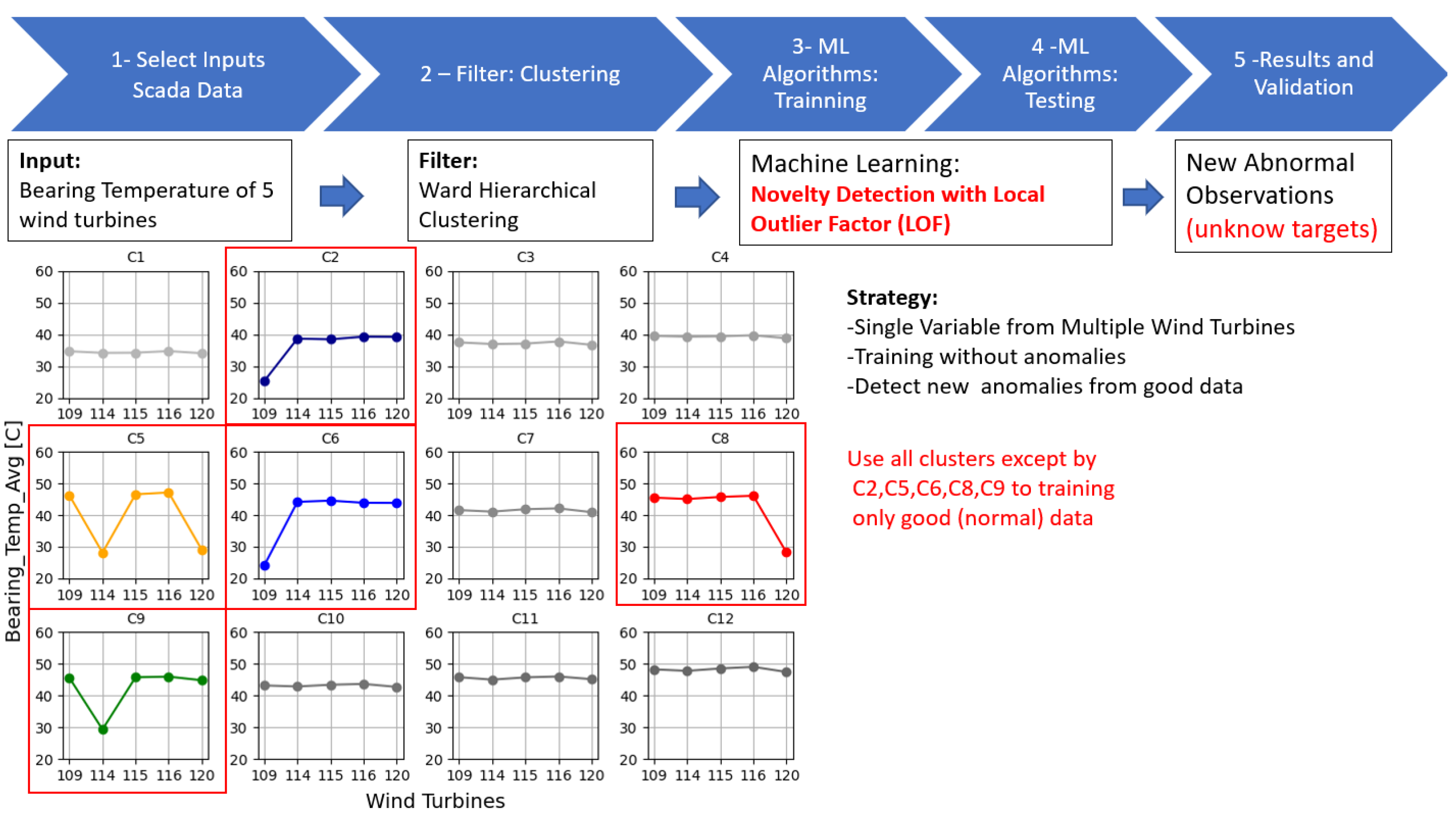
3.1.5. Combined Ward Hierarchical Clustering and Novelty Detection with Local Outlier Factor (WHC-LOF)

This solution uses unsupervised methods to detect turbine failure, where the strategy is to compare simultaneously the variables of a group of wind turbines based on the SCADA data. We chose this method because of time-series independence, which means that the algorithm is able to handle missing data and uses a short time series for training. Figure 5 shows the overview of the methodology. In the first step, we used the complete time series of the bearing temperature of the five wind turbines as an input. Secondly, the data are filtered by removing the events where the bearing temperatures of the five wind turbines are not the same magnitude. The Ward Hierarchical Clustering algorithm [22] was able to identify these events by the clusters C2, C5, C6, C8, and C9, which were manually removed. Then, only the events with the same magnitude of the bearing temperature were used for training. Hence, we used the Novelty Detection with Local Outlier Factor (LOF) [23] with these training data to detect the outliers associated with the failures of the wind turbine (third step). Finally, the algorithm can identify any event where one of the turbines is different from the others as the LOF is trained with only the events with the same magnitude of the bearing temperature.

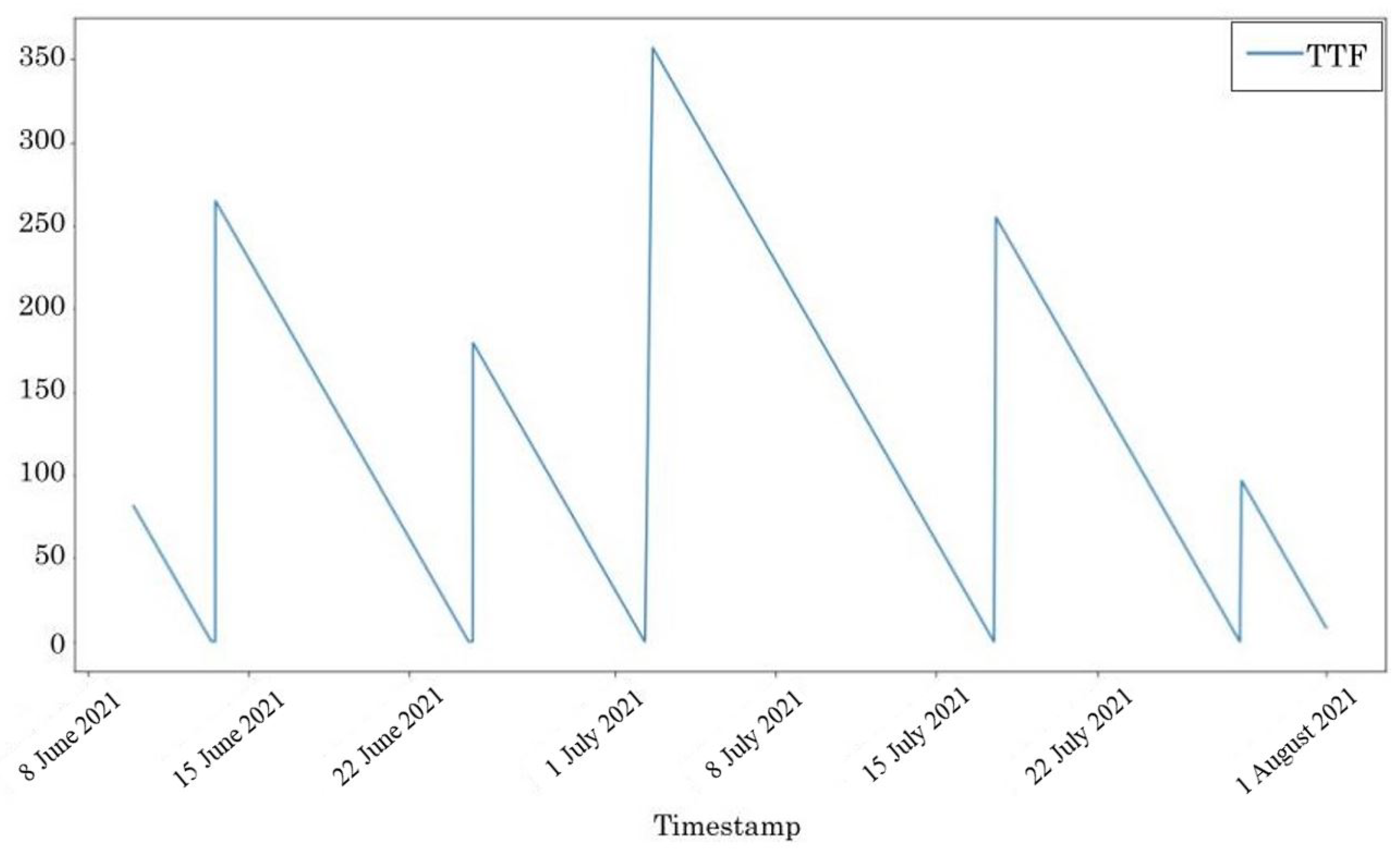
3.1.6. Time-to-Failure Prediction through Random Forest Regression (TTF-RFR)

This solution pre-processes data to create a new variable, referred to as time-to-failure (TTF), which determines the time to failure of the gearbox. To this end, the data set is modified so that the problem can be treated as a supervised problem. Namely, the following steps are implemented:

• Order all gearbox data sets with the “datetime” column in descending order.
• Iterate through all the rows in every dataset.
• While iterating, identify the first failure (error code = 1) and create the TTF variable with value 0.
• In every subsequent row, input the difference between the previous and actual “datetime” columns in the TTF column. In this case, the difference was stored in hour units.
• Whenever the current row is an error code = 1 row, reset the TTF value to 0.

Following this process for all the available gearbox data sets, this solution resulted in a new TTF variable, which models the remaining time until the next error code = 1 or failure occurrence time. The transformation of the problem from a binary event occurrence prediction into a time-to-failure prediction enables the implementation of RUL estimation models instead of anomaly detection ones. Figure 6 shows the calculated TTF value (in hours) for the gearbox #120, as an example of the TTF prediction variable.

The data set has been further pre-processed in order to remove (i) the data collected while the wind turbines are stopped and (ii) highly correlated variables. This was done because, while a wind turbine is stopped, the data records that there is an error. Because of this, if these time-instants are not pre-processed and discarded, models could learn to distinguish when the wind turbine is stopped and when it is running, rather than learning to distinguish when an error occurs and when it is working correctly. In addition, variables that are highly correlated have been removed to avoid having similar or directly repeated data.

As a result, these are the selected explanatory variables that have been used to predict the TTF of the turbine: wind speed, turbulence intensity, nacelle direction, rotor speed, blade angle, generated power, power factor, ambient temperature, brake temperature, hydraulic oil temperature, bearing temperature, hydraulic pressure, gear pressure, air pressure and humidity.

After the proposed re-formulation of the problem, it is possible to resolve the TTF prediction through a supervised learning strategy. To this end, the next phase comprised training and testing the models. This was carried out following a leave-one-out cross validation methodology. In the training of every model, the data set of one gearbox is left out of the training phase and reserved for validation. After training, the data set of the gearbox left outside the training set was used to measure the testing accuracy of the trained model.

An important detail to note is that only the TTF values under 15 h and above 0 h were used for training the predictive model. Hence, the models were trained to predict the time to failure of the last 15 h of operation, and they did not observe the data rows of the actual failures of the gearboxes. The reason for this filter was to design the regression model to (i) focus on the last hours of operation to maximize the accuracy in the most critical moments and (ii) avoid learning from data rows which contain the occurrence of actual failures and to force to predict the TTF out of normal operation data.

The model used for the prediction step was the Random Forest Regression (RFR) model. RFR has been selected because it has shown excellent performance in various competitions, e.g., [15,47]. RFR is an ensemble of recursive trees [48]. Each tree is generated from a bootstrapped sample and a random subset of descriptors is used at the branching of each node in the tree. RFR creates a large number of trees by repeatedly resampling training data and averaging differences through voting. The RFR model was implemented through the sklearn package in Python [46].

3.2. Results

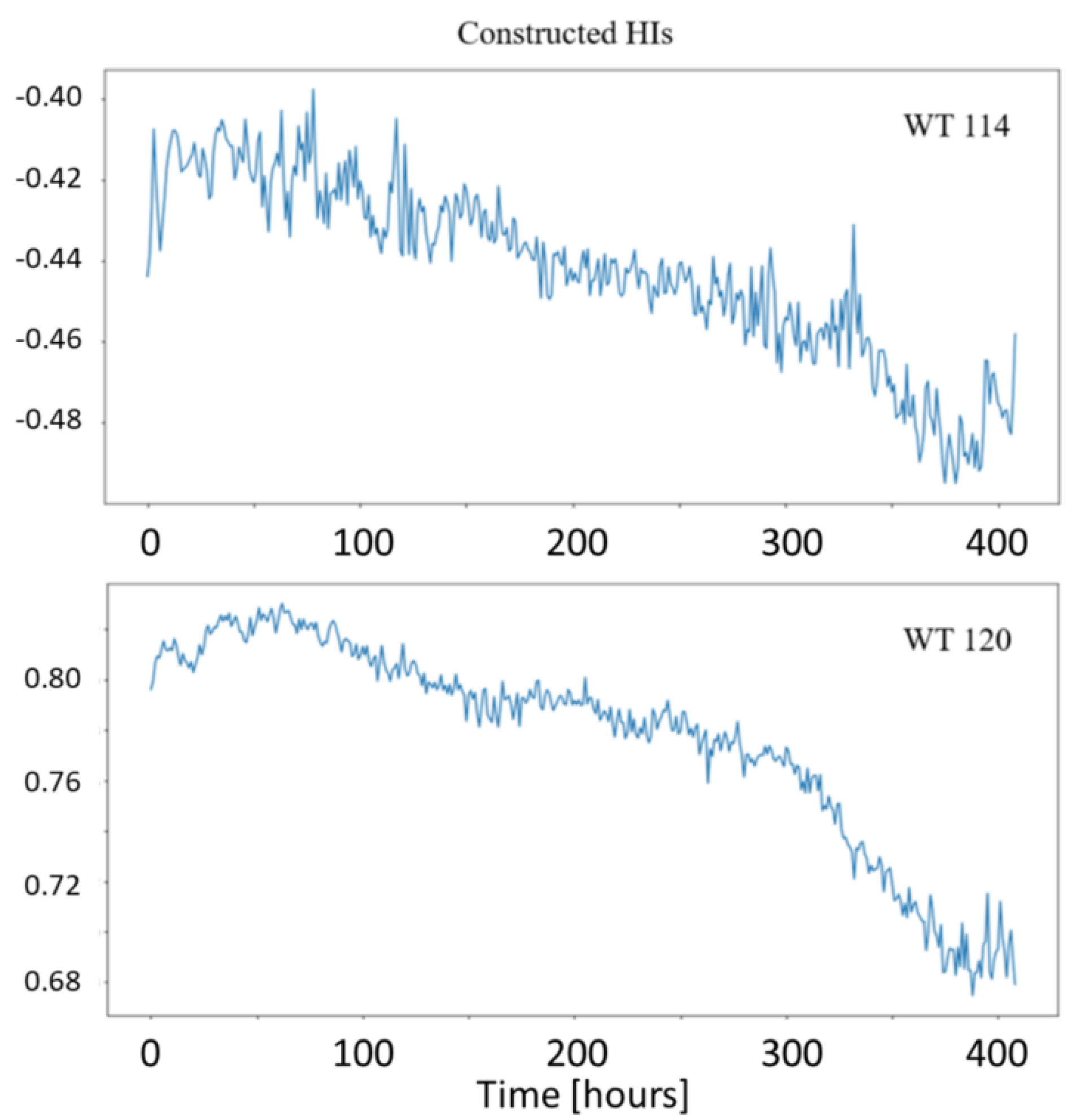
3.2.1. A Convolutional Autoencoder Trained with Particle Swarm Optimisation Algorithm for Constructing Health Indicators (CAE-PSO)

The proposed CAE was trained on the SCADA signals of the last 20 days leading to gearbox failure in wind turbines 114 and 120. The constructed HIs are plotted in Figure 7. Before being fed into the model, the SCADA signals were normalised to a range between 0 and 1 and the data points where the power is negative or the rotational speed is zero were dropped. The results show the ability of the proposed method to construct HIs which are monotonic ($|{\tau }_{MK,114}|=0.7611$, $|{\tau }_{MK,120}|=0.7623$), and, hence, correlated with the expected regime of degradation. Such HIs afford the wind farm operators the possibility to not only detect gearbox failure early, but also to estimate their RUL. However, after training the CAE with one of the two available wind turbine data with gearbox failure, the model is not able to construct a monotonic HI for the other wind turbine, i.e., it does not generalise. The reason is that training the model with only one wind turbine’s data set leads to over-fitting to that specific wind turbine’s operational and environmental conditions around the time of failure. Therefore, to test the performance of this model in predicting the RUL, the model needs to be trained with the data related to several wind turbines experiencing gearbox failure. This could not be done within the scope of this challenge.

3.2.2. Performance Monitoring Using Deep Neural Networks (PM-DNN)

The results of the PM-DNN solution are shown in Figure 8 (top and middle) for an example week for wind turbine number 109 (WTG 109) and WTG 120. nPower refers to normalised power, which is the power divided by the maximum observed power in the data set. Therefore it is dimensionless. A point is flagged as an “Outlier” if the prediction was more than 4 sigma (given by the confidence model) apart from the measurement. A “Warning” is given by a deviation of 3 sigma.

While in Figure 8-middle in some cases there is a accumulation of anomalies about 3 h before the gearbox failure 21, 25, and 26 February 2022), one could assume that the Performance Monitoring approach could work. On the other hand there is no anomaly accumulation before the 22 February 2022, and especially the 23 February 2022. Furthermore, there is an anomaly accumulation on the 24 February 2022 with no following gearbox failure. This trend continues as can be seen in Figure 8-top. There is no significant anomaly accumulation on the 25 February 2022 and there is an accumulation on the 21 February 2022, where no gearbox failure is detected.

While the confusion matrix for WTG 109 is quite sobering (see

Table 2. Confusion matrix for WTG 109 (TP = True Positive, FP = False Positive, TN = True Negative, FN = False Negative; “-” refers to “none”).

TP 71	FN 45
FP 48	TN -

), interestingly the hydraulic oil temperature often spikes in the False Negative cases of the performance monitoring (see Figure 8-bottom). On the other hand, we obtain numerous oil temperature spikes without any gearbox failure. By combining these two approaches one would increase the True Positive rate but would destroy the False Positive rate.

Overall, we conclude that there are at least two kinds of gearbox failures; one which could perhaps be tracked with performance monitoring and the other by monitoring the hydraulic oil temperature. Since it is not known what kind of gearbox failures exist in the data, this is difficult to know for certain. Thus, we have to conclude that there is no systematic appearance of outliers by the performance monitoring before the occurrence of gearbox failures. Therefore, the model cannot be used for prediction purposes, because True Positive rate is too low for a reliable predictor and the combination with oil temperature monitoring would result in an unfeasible high True Negative rate.

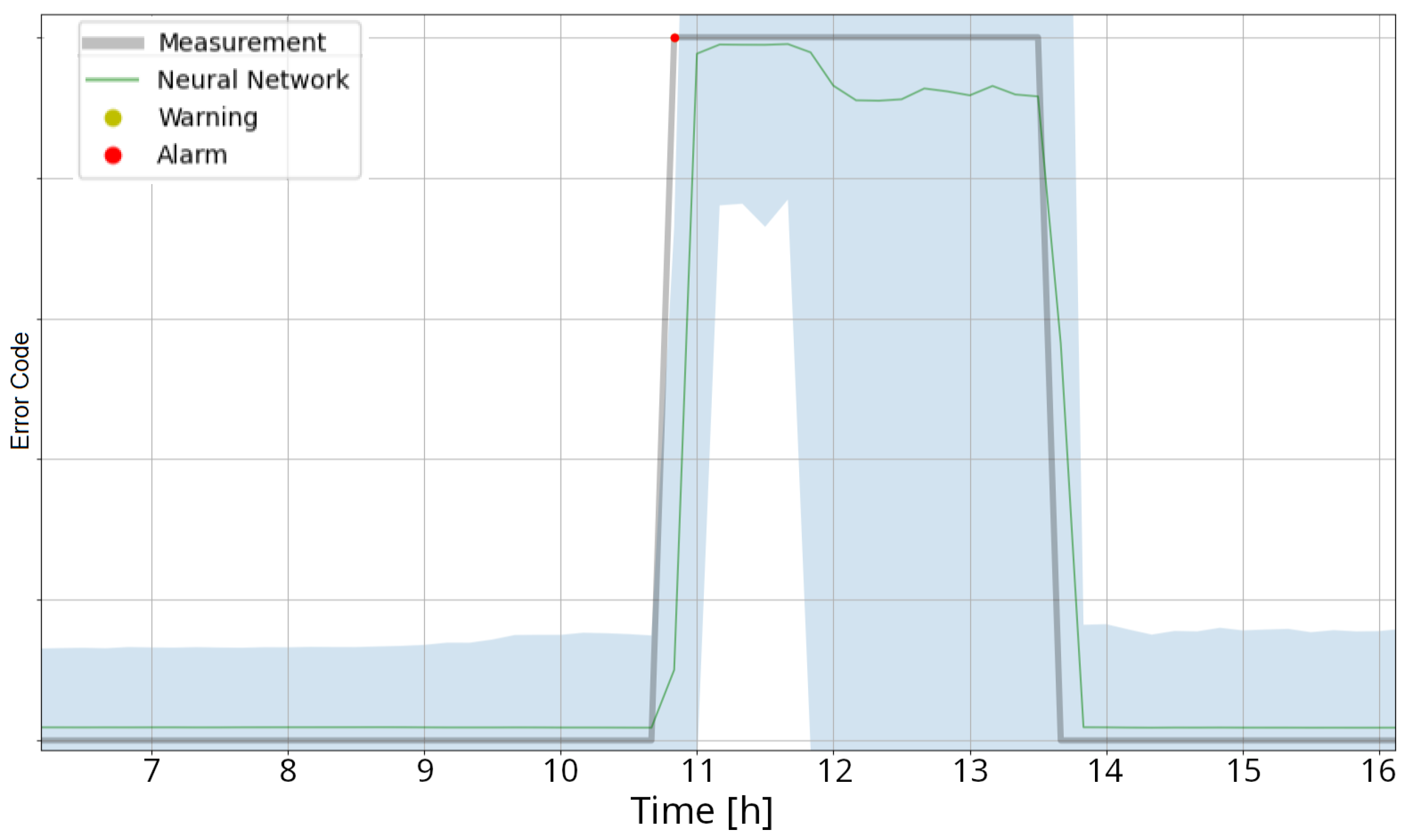
3.2.3. Direct Error Code Prediction Using DNNs (DEC-DNN)

The naive direct approach worked surprisingly well, as can be seen in Figure 9. However, it had a problem where the error codes could not be predicted in advance. In fact, quite the opposite was observed. There are several examples where the error could only be predicted one time step too late (see Figure 10). The conclusion is that the gearbox failures are not predicted by precursors of the failures but by inputs that are consequences of the failure. This could perhaps be enhanced by clustering, or feature engineering, as discussed in the next solution.

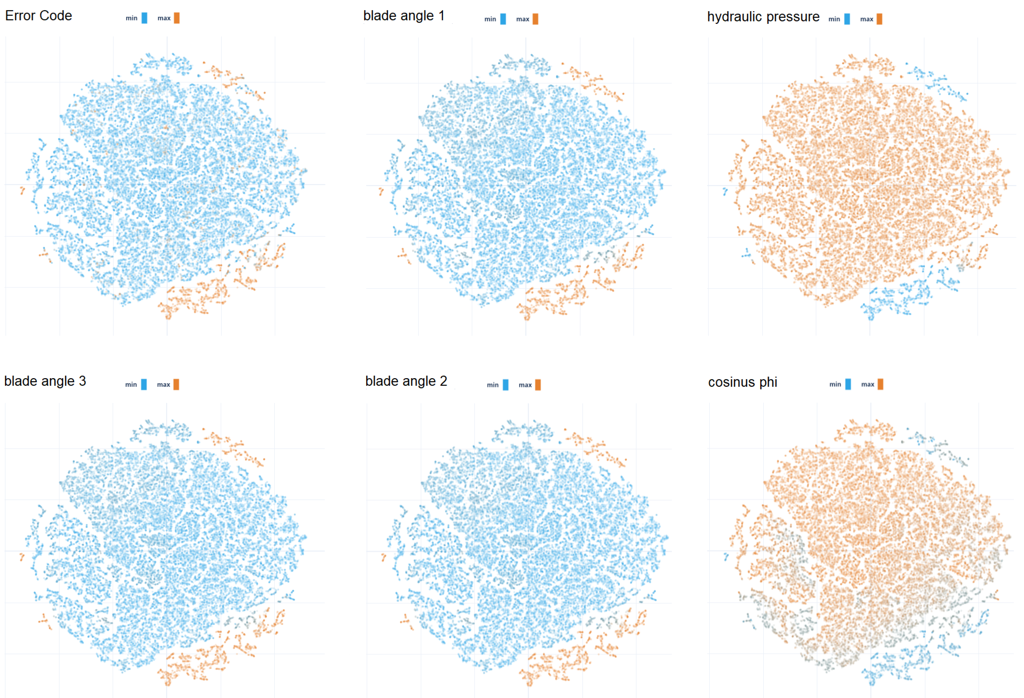
3.2.4. T-SNE Projection for Clustering (T-SNE)

Due to the results in Section 3.2.3, it is interesting to analyse the correlation between different inputs and the error codes, in order to investigate which of the higher correlated inputs are deemed precursors by wind energy experts. The ErrorCode = 1data points cluster well in a few distinct regions as shown in Figure 11. Several input variables are highly correlated with these clusters that represent high gearbox failure probability. However, the shown inputs with high correlation are all consequences of a gearbox failure, not causes. An interesting future work, in the case of the pure T-SNE projection (Section 3.1.4), would be to remove all the variables that experts think are consequences of the failure from the projection and see if the clearly structured clusters of failures are still present. This could indicate a correlation of some inputs to a gearbox failure. This would also make any connections between the remaining inputs to the error codes clearer and could provide a basis for constructing more meaningful features (Feature Engineering). This could be used as a pre-processing method for the other models presented here in the future. With the work done so far one has to assume, however, that this method is not sufficient to predict gearbox failures.

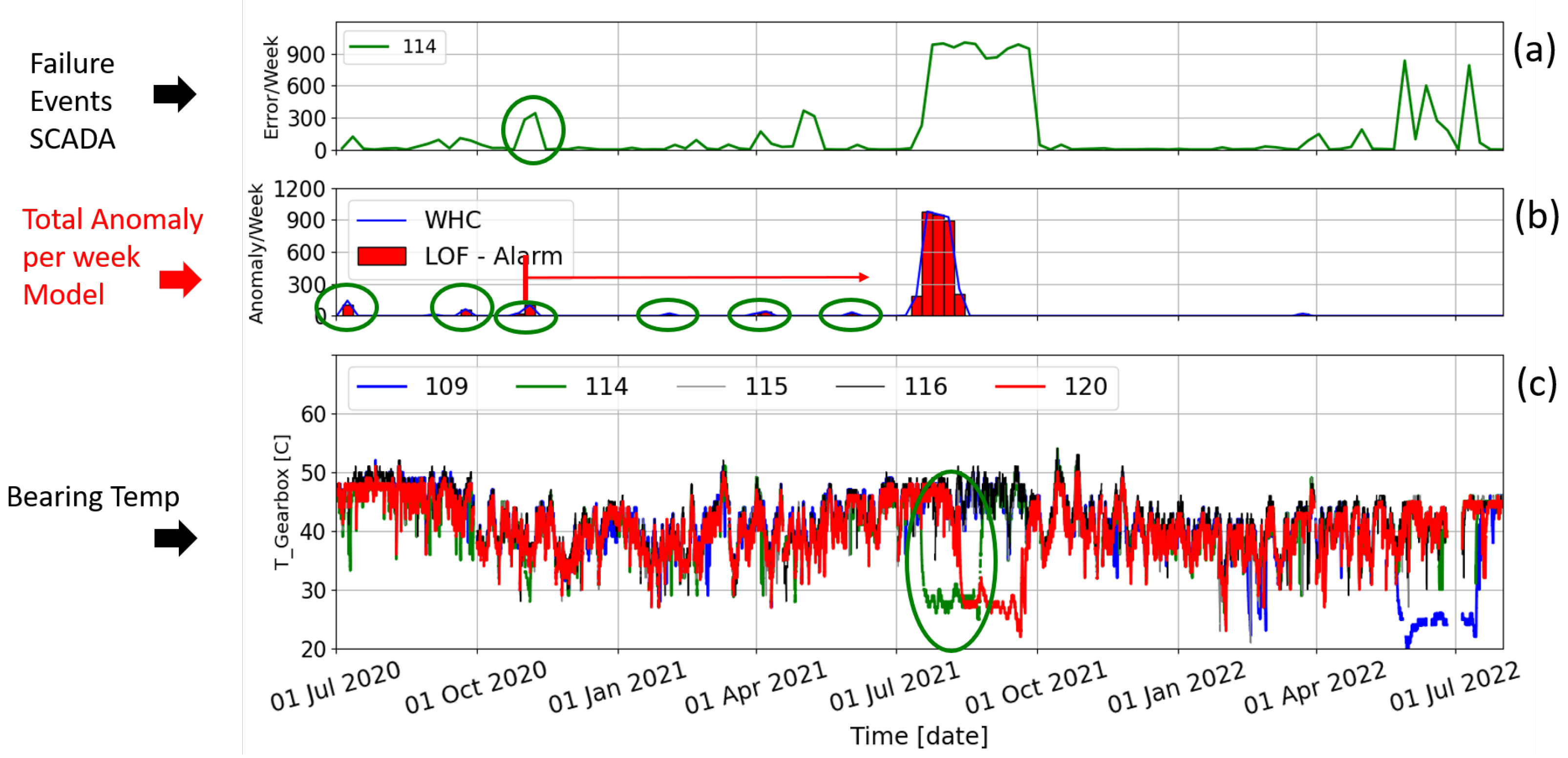
3.2.5. Combined Ward Hierarchical Clustering and Novelty Detection with Local Outlier Factor (WHC-LOF)

Figure 12c shows the time series of temperature bearing of five wind turbines where WTG 114 (green), 109 (blue), and 120 (red) have failed, indicated by the temperature drops along the period, when the turbine stops operating. The WHC-LOF method was applied with the temperature bearing of those five wind turbines, and the anomalies events were considered only for WTG114. The time resolution of the alarm output is important to adjust according to the number of anomalies events accumulated by the turbine. If the time resolution is small, the WHC-LOF can indicate many False Positive (FP) alarms because of the small random anomalies associated with noises of the measurements and the normal variability of the turbine and external conditions (Figure 12a). Thus, after a sensitivity analysis of the time resolution, the WHC-LOF was configured to sum the anomalies events every week (Figure 12b), where a few weekly accumulations of anomaly events are observed before the turbine failure. They may be interpreted in two different ways. First, we have a FP alarm if compared with the same amount of accumulated error code weekly (Figure 12a) with an arbitrary threshold to trigger the alarm. Second, the significant anomalies accumulation in week bases may be considered as a prediction alarm associated with a failure event in the future with a True Positive alarm (TP). However, the presence of an expert is necessary to supervise the anomalies and indicate if it is a possible future failure of the wind turbine.

In Figure 12b, six FP alarms systematically indicate that the turbine has anomalies in its bearing temperature from July 2020 to July 2021. The possible TP alarm may be considered on 8 November 2020 with 103 anomalies/week detected by the WHC-LOF in agreement with a significant number of error codes (341) indicated by the SCADA (Figure 12a). The failure of wind turbine 114 occurred on 18 July 2021, and therefore, the prediction alarm corresponds to 252 days before the turbine failure. The method positively demonstrates the prediction failure of wind turbine 114, which is necessary to understand the behaviour of the wind turbine for a long period before the turbine failure and not just the exact instant that turbine failure. The same method was applied to the EDP Wind Turbine Fault Detection Challenge [3], where the behaviour of the turbines was different from this current challenge, with only one FP detected before the turbine failure. Therefore, the complexity and variety of the behaviours before the turbine’s failure demand more data sets for training the Machine Learning algorithm and for the expert to understand and learn different FPs that may be considered as TP alarms and take the right decision to prevent the turbine failure.

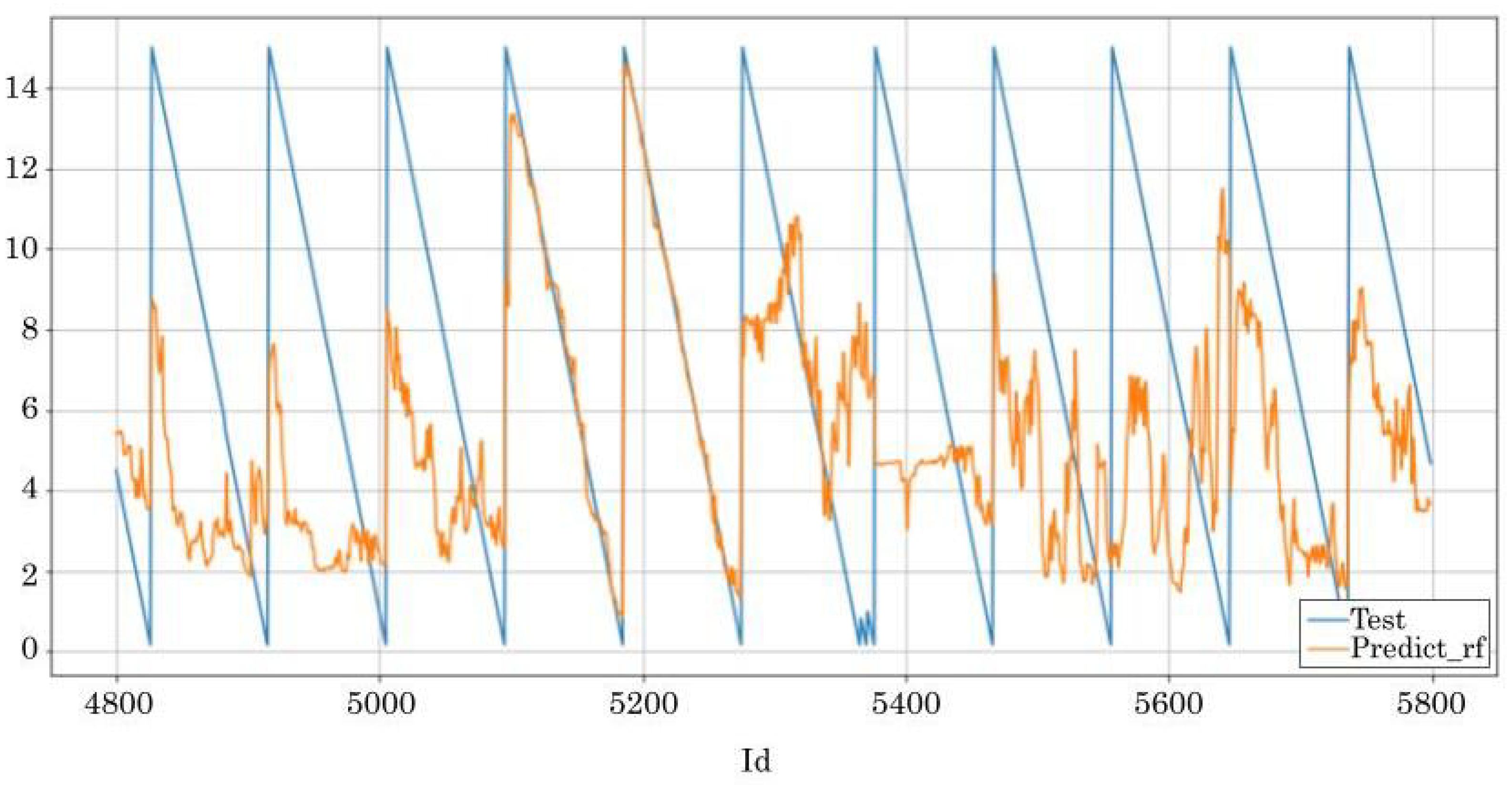
3.2.6. Time-to-Failure Prediction Using Random Forest Regression (TTF-RFR)

Model tuning was performed by adjusting the number of trees in the final model (n_estimators), maximum depth of the tree (max_depth), and the number of features to consider when searching for the best split (max_features). These parameters were evaluated in a predefined grid of parameters. In the first iteration n_estimators was tested in the range [100, 250, 500, 750, 1000, 1500] and in the second iteration it was fine-tuned in the range n_estimators = [700, 750, 800, 850, 900] as well as max_depth = [3, 5, 7, 10, 15, 25] and max_features = [sqrt, log, auto, float, int]. The RFR hyperparameters were tuned, and the best values are obtained with n_estimators = 850, max_depth = 5 and max_features = sqrt, while leaving the remainder of hyperparameters with their default values.

Table 3. Performance statistics of the TTF prediction strategy.

Gearbox Left Out for Testing	MAE (h)
115	3.72
116	3.57
120	3.68
109	3.83
114	3.76

shows the mean absolute error (MAE) of the best model in every run of the cross-validation process.

Figure 13 illustrates an example of the predictions of our model, where the y-axis is the time-to-failure in hours and x-axis is the temporal axis. The blue line is the actual TTF of the gearbox and the orange line is the prediction of the model. In some cases, such as observations 5000–5400, the model was able to predict the overall behaviour of the TTF variable, whereas in other cases, such as observations 5400–5700, it was not. Therefore, the proposed approach could be a practical TTF estimation solution, if the RFR model captures the underlying ageing process, which is not always the case.

All in all, if more information about underlying failure modes were provided, the proposed TTF-RFR approach may be a practical TTF estimate solution through capturing the ageing trajectories and their dependencies. In the current format, only the failure occurrence instants were provided, and with this information, it is challenging to accurately characterise the gearbox time-to-failure.

3.3. Comparison and Evaluation of Solutions

In general, as discussed in detail in [3], the evaluation of time-series anomaly detection algorithms presents a difficult task. This is due to the sensitivity of the algorithm performance to the alarm threshold [49] as well as the fact that false and missed alarms can have very different implications. For SCADA-data-based wind turbine fault detection, the most common measures include root mean squared error (RMSE) [50], mean absolute percentage error (MAPE) [51] and mean absolute error (MAE). Classification models are usually evaluated using accuracy, sensitivity, specificity and F1 [16,52,53]. However, these measures do not account for the costs associated with inspections, repairs and replacements. As this step is highly specific to the asset owner, there is no agreed-upon method for doing this in the literature. In the EDP Challenge, a simple method for estimating costs of True positives (TP), False negatives (FN) and False positives (FP) for different wind turbine components was applied [3].

In this work, a direct comparison using one of these indicators proved impossible, due to the heterogeneous nature of the different solutions. A summary of the main results and learning outcomes related to each solution related to the goal of the Challenge is shown in

Table 4. Summary of main results and learning outcomes.

Solution	Summary of Main Results	Learning Outcomes Related to Data Sharing
CAE-PSO	HIs correlate with degradation, therefore can be used for early failure detection and RUL estimation. However, the result was not generalisable to other wind turbines. The model needs to be trained with data of several wind turbines.	More data sets are required from multiple WTGs experiencing gearbox failure.
PM-DNN	No systematic appearance of outliers before the occurrence of gearbox failures. The model cannot be used for prediction purposes, because True Positive rate is too low for a reliably predictor and the combination with oil temperature monitoring would result in an unfeasibly high True Negative rate.	More information about the optimisation goals (i.e., costs of TPs, FPs and FNs) are needed. More details of failure types are required.
DEC-DNN	The gearbox failures were not predicted by precursors of the failures but by inputs that are consequences of the failure.	None.
T-SNE	Several input variables were highly correlated with these clusters that represent high gearbox failure probability. The shown inputs with high correlation are all consequences of a gearbox failure, not causes. The method is therefore not sufficient to predict gearbox failures.	More details of failure types and detailed analysis with experts needed.
WHC-LOF	The method has potential but the complexity and variety of the behaviours before the turbine’s failure demand more data sets for training the algorithm and for the expert to understand and learn different FPs that may be considered as TP alarms and take the right decision to prevent the turbine failure.	More details of failure types and detailed analysis with experts needed.
TTF-RFR	With the information provided here, it was challenging to accurately characterise the gearbox time-to-failure. Time to failure could be predicted with MAE of 3.57–3.72 h. If more information about underlying failure modes were provided, the approach may be a practical solution through capturing the ageing trajectories and their dependencies.	More details of failure types and detailed analysis with experts needed.

. The goal of the Challenge was to “train, test and validate methods that will provide clear indicators of an upcoming gearbox-related fault, as well as/or a horizon-based probability of the event occurring”. WinJi wanted to “push the performance of such predictions to at least a monthly horizon”. However, the summary presented in Table 4 shows that the submitted solutions did not achieve this directly.

In general, it can be concluded that the CAE-PSO, the PM-DNN, the WHC-LOF and the TTF-RFR solutions appear to have high potential to reach the goals of the challenge. However, there are a number of concrete things that would need to be done by the Challenge Providers:

• Access to more details of the different failure types. This could be performed in future WeDoWind Challenges; however, a trade-off needs to be made by Challenge Providers between anonymising the data and providing enough information to allow the challenge to be completed.
• Access to multiple data sets from more WTGs experiencing gearbox failure. Again, this could be done in future WeDoWind Challenges; however, in this case a decision balancing the amount of provided data and the expected quality of the results needs to be made by the Challenge Provider.
• Provision of a model or rule relating fault detection times or remaining useful lifetime to the estimated costs for repairs, replacements and inspections similar to the EDP one mentioned in Section 3.3. This could be done by the Challenge Provider in the future. Alternatively, this could even be developed by Solution Providers at the start of a Challenge, and facilitated by the moderator.
• Provision of a clear strategy for training and test periods in advance, as is common on other challenge-based platforms such as Kaggle (and as was the case in the previous WeDoWind EDP Challenge), by providing separate training and test data, or by defining how the participants should choose training and test data. In the future, if this is not provided by the Challenge Provider, it could be decided by the participants, and facilitated by the moderator.
• Participation in the Challenge by the Challenge Providers, and provision of details of their results and a description of their method. This can be recommended by the moderators at the start of a WeDoWind Challenge in the future. If there are confidentiality issues, they can take part in a reduced capacity, i.e., by only providing limited results.
• Provision of a pre-defined template or requirements, and even a pre-written analysis code, in order to improve the comparison process. This can be provided by Challenge Providers in future WeDoWind Challenges.

Additionally, the WeDoWind Challenge moderator could have supported this process more actively, as well as focused more on keeping the exact goal of the challenge in sight during the Challenge running.

It can be concluded that there are a number of issues and difficulties that come up when an attempt is made to share data for the purpose of comparing and evaluating different SCADA-data-based wind turbine fault detection models, such as in this WeDoWind Challenge study. This work has allowed a set of best practice data sharing guidelines to be developed, as described below in Section 4.1.

4. Discussion and Outlook

In this section, a new set of best practice data sharing guidelines for wind turbine fault detection model evaluation are first introduced. After that, the WeDoWind framework is evaluated and discussed, both in terms of its applicability here as well as its future transferability to other sectors.

4.1. Best Practice Data Sharing Guidelines for Wind Turbine Fault Detection Model Evaluation

The results of this study have been used to develop a new set of best practice data sharing guidelines, which can be applied directly by practitioners, as summarised in

Table 5. Best practice data sharing guidelines for wind turbine fault detection model evaluation.

Number	Guideline	Recommendation	Comments
1	Some information can be anonymised or normalised to maintain confidentiality	Wind turbine type, location and rated power are recommended	Reducing faults to binary codes can be very limiting for participants, especially if remaining useful lifetime is required
2	The details provided about failure types should be sufficient enough to allow models to be trained, in order to get the best compromise between information and confidentiality	3-4 fault types are recommended	The “Basic concepts and taxonomy of dependable and secure computing” published by IEEE [54] is useful for describing failure types
3	Sufficient data sets containing multiple failures of various wind turbines should be provided, in order to obtain the best compromise between information and confidentiality	At least 3–4 different faults should occur in 3–4 different wind turbines	-
4	A model or rule relating fault detection times or remaining useful lifetime to the estimated costs for repairs, replacements and inspections should be provided in advance.	A cost model for repairs, replacements and inspections similar to the EDP one is recommended [3].	If this cannot be done, the participants should make sure that this is discussed and agreed on at the start of the challenge.
5	A clear strategy for training and test periods should be provided in advance.	The provided data can be split into training and test data sets in advance.	If this cannot be done, the participants should ensure that this is discussed and agreed on at the start of the challenge.
6	The challenge provider should take part in the challenge.	In the best case, they should share both results and a description of their method.	If there are confidentiality issues, they can take part in a reduced capacity, i.e., by only providing results.
7	The challenge moderator should focus more on the goal of the challenge and actively do things to help the participants reach the goal.	Requiring the results to be submitted in a certain format or providing a template.	An analysis code can also be provided.

.

4.2. Applicability of the WeDoWind Framework

We have shown that the WeDoWind framework can be applied to successfully bring together a pool of talented and diverse people with different backgrounds to collaboratively tackle a problem. It exposes them to the realities of having to deal with unstructured and uncharacterised data, rather than nicely prepared simulation data. While further work is required to use the WeDoWind framework to directly produce easily-applicable open-source code, it nevertheless provides Challenge Providers with new insights and ideas for the improvement of their models. Initial feedback from some of the challenge participants showed that they highly value the possibility provided by WeDoWind to to compare and evaluate their work as well as the webinar organisation, which allowed ideas to be shared and discussed. A thorough participant survey is currently underway. Further case studies with a wide range of partners are underway. Ultimately, this allows the three “Grand Challenges of digitalisation in wind energy” to be addressed in a holistic manner. The results will be used to iteratively enhance and improve the best practice data sharing guidelines.

Some of the limitations that have become apparent during this work include: (a) the lack of a specific method for ensuring that the provided data is of sufficient quality or quantity, or that it is sufficiently documented for solving the challenge, (b) the lack of formal evaluation method defined at the beginning of the Challenges, and (c) the poor usability of the digital platform. Solutions for overcoming these limitations are currently being developed.

4.3. Outlook

The work presented in this paper is transferable to any industry in which data are being used to create business value. The idea of creating challenges that mutually benefit multiple parties can be used in any sector or for any topic. For example, researchers developing energy system planning tools may be interested in comparing and evaluating different tools based on some data provided by local and national authorities. Anyone developing fault detection tools for large structures or operating machines may be interested in comparing their tools based on data provided by the asset owners. Furthermore, the framework could even be applied to help organisations develop more useful and effective medical devices or services that better reflect the needs of patients, by bringing together all the important stakeholders together to solve the largest challenges. It could even be applicable to enhance data sharing and collaboration in political settings, such as by bringing together people from local communities to assess the results of surveys or other public data collection efforts and to provide inputs to the developers of public services.

5. Conclusions

In this work, the challenges related to comparing and evaluating different SCADA-data-based wind turbine fault detection models were investigated by carrying out a new case study, the “WinJi Gearbox Fault Detection Challenge”, based on the WeDoWind framework. The WeDoWind framework has previously been shown to create tangible incentives to motivate and empower different types of people from all over the world to share data and knowledge in practice.

The goal of the challenge was to help WinJi, the Challenge Providers, to push the performance of their predictions to at least a monthly horizon, by making use of the provided SCADA data in order to train, test and validate methods that will provide clear indicators of an upcoming gearbox related fault, as well as/or a horizon-based probability of the event occurring. A total of six new solutions were submitted to the challenge, using approaches including a Convolutional Autoencoder trained with Particle Swarm Optimisation algorithm for constructing health indicators (CAE-PSO), performance monitoring using Deep Neural Networks (PM-DNN), Direct Error Code Prediction using DNNs (DEC-DNN), T-SNE Projection for clustering (T-SNE), Combined Ward Hierarchical Clustering and Novelty Detection with Local Outlier Factor (WHC-LOC) and Time-to-failure prediction using Random Forest Regression (TTF-RFR).

A comparison and evaluation of the results showed that, in general, some of the approaches (CAE-PSO, PM-DNN, WHC-LOF and TTF-RFR) appear to have high potential to reach the goals of the challenge. However, there were a number of concrete things that would first need to done by the challenge providers and the challenge moderators in order to ensure success. This includes enabling access to more details of the different failure types, access to multiple data sets from more WTGs experiencing gearbox failure, provision of a model or rule relating fault detection times or a remaining useful lifetime to the estimated costs for repairs, replacements and inspections, provision of a clear strategy for training and test periods in advance, participation in the challenge and provision of details of their results and description of their method as well as provision of a pre-defined template or requirements.

This work presents some of the difficulties encountered when enabling cooperation between organisations and connecting people and data for a successful implementation of digitalisation in wind energy. Thus, these learning outcomes were employed directly to define a set of best practice data sharing guidelines for wind turbine fault detection model evaluation, in order to improve model evaluation and data sharing in the future.

The work presented in this paper is transferable to any industry in which data are being used to create business value, and case studies are currently being developed in a range of different sectors.

References

1. Clifton, A.; Barber, S.; Bray, A.; Enevoldsen, P.; Fields, J.; Sempreviva, A.M.; Williams, L.; Quick, J.; Purdue, M.; Totaro, P.; et al. Grand Challenges in the Digitalisation of Wind Energy. Wind Energy Sci. 2022. in review. [Google Scholar] [CrossRef]
2. Wilkinson, M.; Dumontier, M.; Aalbersberg, I.; Appleton, G.; Axton, M.; Baak, A.; Blomberg, N.; Boiten, J.-W.; da Silva Santos, L.B.; Bourne, P.E.; et al. The FAIR Guiding Principles for scientific data management and stewardship. Sci. Data 2016, 3, 160018. [Google Scholar] [CrossRef]
3. Barber, S. Co-Innovation for a Successful Digital Transformation in Wind Energy Using a New Digital Ecosystem and a Fault Detection Case Study. Energies 2022, 15, 5638. [Google Scholar] [CrossRef]
4. Maria, S.A.; Allan, V.; Christian, B.; Robert, V.D.; Gregor, G.; Kjartansson, D.H.; Pilgaard, M.L.; Mattias, A.; Nikola, V.; Stephan, B.; et al. Taxonomy and Metadata for Wind Energy Research & Development. Zenodo, 12 December 2017. [Google Scholar] [CrossRef]
5. Barber, S.; Clark, T.; Day, J.; Totaro, P. The IEA Wind Task 43 Metadata Challenge: A Roadmap to Enable Commonality in Wind Energy Data. Zenodo, 4 April 2022. [Google Scholar] [CrossRef]
6. Bresciani, S.; Ciampi, F.; Meli, F.; Ferraris, A. Using big data for co-innovation processes: Mapping the field of data-driven innovation, proposing theoretical developments and providing a research agenda. Int. J. Inf. Manag. 2021, 60, 102347. [Google Scholar] [CrossRef]
7. Lee, S.M.; Olson, D.L.; Trimi, S. Co-innovation: Convergenomics, collaboration, and co-creation for organizational values. Manag. Decis. 2012, 50, 817–831. [Google Scholar] [CrossRef]
8. Dao, C.; Kazemtabrizi, B.; Crabtree, C. Wind turbine reliability data review and impacts on levelised cost of energy. Wind Energy 2019, 22, 1848–1871. [Google Scholar] [CrossRef]
9. Zaher, A.; McArthur, S.; Infield, D.; Patel, Y. Online wind turbine fault detection through automated SCADA data analysis. Wind. Energy Int. J. Prog. Appl. Wind. Power Convers. Technol. 2009, 12, 574–593. [Google Scholar] [CrossRef]
10. Butler, S.; Ringwood, J.; O’Connor, F. Exploiting SCADA system data for wind turbine performance monitoring. In Proceedings of the 2013 Conference on Control and Fault-Tolerant Systems (SysTol), Nice, France, 9–11 October 2013; pp. 389–394. [Google Scholar]
11. Kusiak, A.; Verma, A. Analyzing bearing faults in wind turbines: A data-mining approach. Renew. Energy 2012, 48, 110–116. [Google Scholar] [CrossRef]
12. Sun, P.; Li, J.; Wang, C.; Lei, X. A generalized model for wind turbine anomaly identification based on SCADA data. Appl. Energy 2016, 168, 550–567. [Google Scholar] [CrossRef]
13. Bangalore, P.; Letzgus, S.; Karlsson, D.; Patriksson, M. An artificial neural network-based condition monitoring method for wind turbines, with application to the monitoring of the gearbox. Wind. Energy 2017, 20, 1421–1438. [Google Scholar] [CrossRef]
14. Bach-Andersen, M.; Rømer-Odgaard, B.; Winther, O. Flexible non-linear predictive models for large-scale wind turbine diagnostics. Wind Energy 2017, 20, 753–764. [Google Scholar] [CrossRef]
15. Liu, Y.; Chen, H.; Zhang, L.; Feng, Z. Enhancing building energy efficiency using a random forest model: A hybrid prediction approach. Energy Rep. 2021, 7, 5003–5012. [Google Scholar] [CrossRef]
16. Stetco, A.; Dinmohammadi, F.; Zhao, X.; Robu, V.; Flynn, D.; Barnes, M.; Keane, J.; Nenadic, G. Machine learning methods for wind turbine condition monitoring: A review. Renew. Energy 2019, 133, 620–635. [Google Scholar] [CrossRef]
17. Schlechtingen, M.; Santos, I.F. Comparative analysis of neural network and regression based condition monitoring approaches for wind turbine fault detection. Mech. Syst. Signal Process. 2011, 25, 1849–1875. [Google Scholar] [CrossRef]
18. Fu, J.; Chu, J.; Guo, P.; Chen, Z. Condition Monitoring of Wind Turbine Gearbox Bearing Based on Deep Learning Model. IEEE Access 2019, 7, 57078–57087. [Google Scholar] [CrossRef]
19. Gougam, F.; Rahmoune, C.; Benazzouz, D.; Varnier, C.A.C.; Nicod, J.M. Health Monitoring Approach of Bearing: Application of Adaptive Neuro Fuzzy Inference System (ANFIS) for RUL-Estimation and Autogram Analysis for Fault-Localization. In Proceedings of the 2020 Prognostics and Health Management Conference (PHM-Besançon), Besancon, France, 4–7 May 2020; pp. 200–206. [Google Scholar]
20. Li, X.; Teng, W.; Peng, D.; Ma, T.; Wu, X.; Liu, Y. Feature fusion model based health indicator construction and self-constraint state-space estimator for remaining useful life prediction of bearings in wind turbines. Reliab. Eng. Syst. Saf. 2023, 233, 109124. [Google Scholar] [CrossRef]
21. Xu, Z.; Bashir, M.; Liu, Q.; Miao, Z.; Wang, X.; Wang, J.; Ekere, N. A novel health indicator for intelligent prediction of rolling bearing remaining useful life based on unsupervised learning model. Comput. Ind. Eng. 2023, 176, 108999. [Google Scholar] [CrossRef]
22. Ward, J.H. Hierarchical Grouping to Optimize an Objective Function. J. Am. Stat. Assoc. 1963, 58, 236–244. [Google Scholar] [CrossRef]
23. Breunig, M.; Kriegel, H.P.; Ng, R.T.; Sander, J. LOF: Identifying Density-Based Local Outliers. In Proceedings of the 2000 Acm Sigmod International Conference On Management Of Data, Dallas, TX, USA, 16–18 May 2000; pp. 93–104. [Google Scholar]
24. Ahmed, I.; Dagnino, A.; Ding, Y. Unsupervised Anomaly Detection Based on Minimum Spanning Tree Approximated Distance Measures and its Application to Hydropower Turbines. IEEE Trans. Autom. Sci. Eng. 2019, 16, 654–667. [Google Scholar] [CrossRef]
25. Dao, P.B. A CUSUM-Based Approach for Condition Monitoring and Fault Diagnosis of Wind Turbines. Energies 2021, 14, 3236. [Google Scholar] [CrossRef]
26. Xu, Q.; Lu, S.X.; Zhai, Z.; Jiang, C. Adaptive fault detection in wind turbine via RF and CUSUM. IET Renew. Power Gener. 2020, 14, 1789–1796. [Google Scholar] [CrossRef]
27. Li, G.; Shi, J. Applications of Bayesian methods in wind energy conversion systems. Renew. Energy 2012, 43, 1–8. [Google Scholar] [CrossRef]
28. Zhang, C.; Liu, Z.; Zhang, L. Wind turbine blade bearing fault detection with Bayesian and Adaptive Kalman Augmented Lagrangian Algorithm. Renew. Energy 2022, 199, 1016–1023. [Google Scholar] [CrossRef]
29. Meng, L.; Su, Y.; Kong, X.; Lan, X.; Li, Y.; Xu, T.; Ma, J. A Probabilistic Bayesian Parallel Deep Learning Framework for Wind Turbine Bearing Fault Diagnosis. Sensors 2022, 22, 7644. [Google Scholar] [CrossRef] [PubMed]
30. Pandit, R.; Astolfi, D.; Hong, J.; Infield, D.; Santos, M. SCADA data for wind turbine data-driven condition/performance monitoring: A review on state-of-art, challenges and future trends. Wind Eng. 2023, 47, 422–441. [Google Scholar] [CrossRef]
31. Astolfi, D.; Pandit, R.; Terzi, L.; Lombardi, A. Discussion of Wind Turbine Performance Based on SCADA Data and Multiple Test Case Analysis. Energies 2022, 15, 5343. [Google Scholar] [CrossRef]
32. Maron, J.; Anagnostos, D.; Brodbeck, B.; Meyer, A. Artificial intelligence-based condition monitoring and predictive maintenance framework for wind turbines. J. Phys. Conf. Ser. 2022, 2151, 012007. [Google Scholar] [CrossRef]
33. Pohlert, T. Non-Parametric Trend Tests and Change-Point Detection. Thorsten Pohlert. 24 March 2015. Available online: https://www.researchgate.net/publication/274014742_trend_Non-Parametric_Trend_Tests_and_Change-Point_Detection_R_package_version_001?channel=doi&linkId=551298ec0cf268a4aaea93c9&showFulltext=true (accessed on 10 April 2023).
34. Poli, R.; Kennedy, J.; Blackwell, T. Particle swarm optimization. Swarm Intell. 2007, 1, 33–57. [Google Scholar] [CrossRef]
35. Faris, H.; Aljarah, I.; Mirjalili, S. Training feedforward neural networks using multi-verse optimizer for binary classification problems. Appl. Intell. 2016, 45, 322–332. [Google Scholar] [CrossRef]
36. Mazurowski, M.A.; Habas, P.A.; Zurada, J.M.; Lo, J.Y.; Baker, J.A.; Tourassi, G.D. Training neural network classifiers for medical decision making: The effects of imbalanced datasets on classification performance. Neural Netw. 2008, 21, 427–436. [Google Scholar] [CrossRef]
37. Zhang, Y.M.; Wang, H.; Mao, J.X.; Xu, Z.D.; Zhang, Y.F. Probabilistic Framework with Bayesian Optimization for Predicting Typhoon-Induced Dynamic Responses of a Long-Span Bridge. J. Struct. Eng. 2021, 147, 04020297. [Google Scholar] [CrossRef]
38. Jha, G.K.; Thulasiraman, P.; Thulasiram, R.K. PSO based neural network for time series forecasting. In Proceedings of the 2009 International Joint Conference on Neural Networks, Atlanta, GA, USA, 14–19 June 2009. [Google Scholar] [CrossRef]
39. Schmidhuber, J. Deep Learning in Neural Networks: An Overview. Neural Netw. 2015, 61, 85–117. [Google Scholar] [CrossRef] [PubMed]
40. Kingma, D.P.; Ba, J. Adam: A method for stochastic optimization. arXiv 2014, arXiv:1412.6980. [Google Scholar]
41. Paszke, A.; Gross, S.; Massa, F.; Lerer, A.; Bradbury, J.; Chanan, G.; Killeen, T.; Lin, Z.; Gimelshein, N.; Antiga, L.; et al. PyTorch: An Imperative Style, High-Performance Deep Learning Library. In Advances in Neural Information Processing Systems 32; Curran Associates, Inc.: Red Hook, NY, USA, 2019; pp. 8024–8035. [Google Scholar]
42. Sehnke, F.; Osendorfer, C.; R’uckstieß, T.; Graves, A.; Peters, J.; Schmidhuber, J. Parameter-exploring policy gradients. Neural Netw. 2010, 23, 551–559. [Google Scholar] [CrossRef]
43. Sehnke, F. Efficient baseline-free sampling in parameter exploring policy gradients: Super symmetric pgpe. In Proceedings of the International Conference on Artificial Neural Networks, Sofia, Bulgaria, 10–13 September 2013; pp. 130–137. [Google Scholar]
44. Sehnke, F.; Zhao, T. Baseline-free sampling in parameter exploring policy gradients: Super symmetric pgpe. In Artificial Neural Networks; Springer: Berlin/Heidelberg, Germany, 2015; pp. 271–293. [Google Scholar]
45. Van der Maaten, L.; Hinton, G. Visualizing data using t-SNE. J. Mach. Learn. Res. 2008, 9, 2579–2605. [Google Scholar]
46. Pedregosa, F.; Varoquaux, G.; Gramfort, A.; Michel, V.; Thirion, B.; Grisel, O.; Blondel, M.; Prettenhofer, P.; Weiss, R.; Dubourg, V.; et al. Scikit-learn: Machine Learning in Python. J. Mach. Learn. Res. 2011, 12, 2825–2830. [Google Scholar]
47. Nagy, G.I.; Barta, G.; Kazi, S.; Borbély, G.; Simon, G. GEFCom2014: Probabilistic solar and wind power forecasting using a generalized additive tree ensemble approach. Int. J. Forecast. 2016, 32, 1087–1093. [Google Scholar] [CrossRef]
48. Breiman, L. Random forests. Mach. Learn. 2001, 45, 5–32. [Google Scholar] [CrossRef]
49. Ruff, L.; Kauffmann, J.R.; Vandermeulen, R.A.; Montavon, G.; Samek, W.; Kloft, M.; Dietterich, T.G.; Müller, K.R. A Unifying Review of Deep and Shallow Anomaly Detection. Proc. IEEE 2021, 109, 756–795. [Google Scholar] [CrossRef]
50. Orozco, R.; Sheng, S.; Phillips, C. Diagnostic Models for Wind Turbine Gearbox Components Using SCADA Time Series Data. In Proceedings of the 2018 IEEE International Conference on Prognostics and Health Management (ICPHM), Seattle, WA, USA, 11–13 June 2018; pp. 1–9. [Google Scholar] [CrossRef]
51. Wang, L.; Zhang, Z.; Long, H.; Xu, J.; Liu, R. Wind Turbine Gearbox Failure Identification With Deep Neural Networks. IEEE Trans. Ind. Inform. 2017, 13, 1360–1368. [Google Scholar] [CrossRef]
52. Arcos Jiménez, A.; Gómez Muñoz, C.Q.; García Márquez, F.P. Machine Learning for Wind Turbine Blades Maintenance Management. Energies 2018, 11, 13. [Google Scholar] [CrossRef]
53. Tang, B.; Song, T.; Li, F.; Deng, L. Fault diagnosis for a wind turbine transmission system based on manifold learning and Shannon wavelet support vector machine. Renew. Energy 2014, 62, 1–9. [Google Scholar] [CrossRef]
54. Avizienis, A.; Laprie, J.C.; Randell, B.; Landwehr, C. Basic concepts and taxonomy of dependable and secure computing. IEEE Trans. Dependable Secur. Comput. 2004, 1, 11–33. [Google Scholar] [CrossRef]
55. Barber, S. GitLab Repository “WeDoWind—WinJi Gearbox Failure Detection”. 2023. [Google Scholar]
Figure 1. The value creation process of the WeDoWind framework.
Energies 16 03567 g001
Figure 2. Power Curve and wind rose for the WT115.
Energies 16 03567 g002
Figure 3. Architecture of the CAE.
Energies 16 03567 g003
Figure 4. Architecture of the Encoder of the CAE. The Decoder is symmetric.
Energies 16 03567 g004
Figure 5. Overview of the WHC-LOF method that combines Ward Hierarchical Clustering (WHC) for the filter process and Novelty Detection with Local Outlier Factor (LOF) for detecting the anomalies where only the good (normal) data is used to train (red text).
Energies 16 03567 g005
Figure 6. TTF estimation for WT #120.
Energies 16 03567 g006
Figure 7. Constructed HIs for WT 114 and 120—last 20 days leading to the gearbox failure.
Energies 16 03567 g007
Figure 8. An example week for the WTG 120 (top) and 109 (middle) with several gearbox error codes. As can be seen for WTG 109, in some cases there is a accumulation of anomalies quite some time before the gearbox failure (21, 25, and 26 February 2022). On the other hand there is no anomaly accumulation before the 22 and especially the 23 February 2022. Furthermore, there is an anomaly accumulation at the 24 February 2022 with no following gearbox failure. Temperature of the hydraulic oil (bottom) is however spiking before the 22. The same week as for the WTG 109 is shown for the WTG 120. There is no significant anomaly accumulation on the 25 February 2022 and there is an accumulation on the 21 February 2022, where no gearbox failure is detected. nPower refers to normalised power, which is the power divided by the maximum observed power in the data set.
Energies 16 03567 g008
Figure 9. The direct modelling of the error codes leads to a model that can predict the gearbox failures very well as they happen but not in advance. This can be seen by the DNN (green line) following the error code (grey line) closely.
Energies 16 03567 g009
Figure 10. Sometimes the model can even predict the gearbox failure one time step too late. This can be seen in the shown instance there the error code appears 10 min before the DNN predicted likelihood for an error code goes up.
Energies 16 03567 g010
Figure 11. T-SNE projection of error codes and inputs into a 2D space. The error codes cluster well in a few distinct regions and some inputs show high correlation to these clusters. However, all inputs that were identified by this method are consequences of a gearbox failure not a cause.
Energies 16 03567 g011
Figure 12. Error code from the SCADA data when the Turbine 114 indicates possible failures, with the data accumulated every week (a), Failure of Turbine 114 detected by WHC-LOF method with data accumulated every week (b), Time series of the bearing temperature of the five wind turbines where the green circle indicates that the bearing temperature drops when the Turbine 114 fails (c).
Energies 16 03567 g012
Figure 13. Difference between real and predicted TTF values for WT #109.
Energies 16 03567 g013