District Heating System Optimisation: A Three-Phase Thermo-Hydraulic Linear Model

Abstract

Investments in the development of the district heating system require a thorough analysis of the technical, economic, and legal aspects. Regarding the technical and economic context, a mathematical model of the district heating system has been proposed. It optimizes both the technical and economic aspects of the function and development of a district heating system. To deal with non-linearities, the developed linear programming model is divided into three phases: flow, thermal, and pressure. Therein, non-linear dependencies are calculated between the linear optimization phases. This paper presents the main assumptions and equations that were used to calculate the parameters of the heating system, along with the optimal level of heat production, the flow rate of the heating medium in the heat nodes and edges of the network graph, the heat, power, and temperature losses at each edge, and the purchase costs of heat and its transmission. The operation of the model was tested on a real-world district heating system. The case study results confirm that the model is effective and can be used in decision support. The economic results of the model, before the calibration process, were 3.6% different from historical values. After the calibration process, they were very similar to the real data—all percentage deviations were within 1%.

1. Introduction

Poland is among the European leaders in terms of the percentage of inhabitants connected to and who acquire heat through the district heating system. Over 50 percent of inhabitants are supplied through the district heating system. Poland is among the European leaders in terms of the percentage of inhabitants connected to and who acquire heat through the district heating system. Over 40 percent of inhabitants are supplied from the district heating system. Poland is the 6th largest district heating producer in terms of its share of consumers after Iceland (almost 100%), Latvia, Denmark, Lithuania, and Estonia [1]. District heating companies produced 376 PJ of heat in 2018, of which 233.6 PJ was the heat supplied to customers connected to the network [2]. In the face of war in Ukraine and the optimization of heating costs, restructuring of the system can be crucial to further operation. In fact, due to energy efficiency efforts carried out over the last decades, it is very difficult now to maintain the share of district heating relative to the total heat consumption in Poland.

The Polish district heating sector is very diversified. This applies to the network size, as well as to the number of companies operating in particular regions. Moreover, the fuels used for heat generation also vary depending on the location. In some regions (usually located near coal supply regions), over 90 percent of heat is coal-based. By contrast, in other regions, only 13 percent of heat is coal-based, and the heat production is dominated by natural gas (the share is over 80 percent).

Owing to the fact that the district heating system has to compete with other heating sources, the problem of optimization of the operation of this system captures the attention of decision makers. One of the well-known options in the decision-making process is the development of tools that serve as a ’helping hand’ in the process of making strategic and operational decisions.

The remainder of the paper is structured as follows. In Section 2, a literature review is presented. Section 3 contains a detailed description of the developed tool, and the main assumptions for the flow, thermal, and pressure phases are presented. Section 4, covers the description of a case study for which the model validation was conducted. Finally, in Section 5, the main findings are discussed.

2. Literature Review

The development of computational models that are applied in order to support decisions related to expanding or redesigning district heating systems is a complex task. Although the simulation and optimization of the operation of district heating systems have been the subject of several papers, only a few developed models have allowed operational or strategic analyses of district heating systems to be made. The forthcoming paragraphs provide a concise review of achievements in this field.

The authors of [3] presented a model for the thermo-economical optimal design of district heating network topologies with pipe diameter choices and operation parameters for realistic district heating networks. This approach is based on the adjoint approach and works with the possibility complete transport model to deal with the nonlinear effects that characterize 4th generation district heating networks. Owing to optimization based on a nonlinear physics model, heat losses, and the temperature-dependent effectiveness of consumer heating, systems could already be calculated in the design phase. The objective function was to minimize the costs associated with installed network piping, installed pump capacity, and its operation while meeting the thermal demand of all consumers within a reasonable tolerance.

In [4], the authors proposed an optimizing tool to find the correct district heating network expansion strategy under specified constraints. The model developed in the paper was formulated using a mixed-integer linear programming approach. The optimization problem was developed through the General Algebraic Modelling System (GAMS). The goal of the proposed model was that the future network extension be optimized based on the existing network’s capacities and layout, as well as on realistic connection scenarios and constraints identified by users. The objective function concerns regarded cost savings maximization or greenhouse gas emissions minimization. The model selected from the best mix of technologies and pipeline connection strategies to achieve that purpose.

A tool for the strategic outline and sizing of district heating networks using a geographic information system was developed in [5]. This study was developed based on a multi-period mixed-integer linear programming (MILP) optimization model that was part of a decision tool to optimally outline and size any new heating network project. This model aimed to maximize the net cash flow from a heating network while accounting for a few constraints (the main physical and urbanistic issues). Furthermore, the model enabled the ability to take into account the temporal behavior of the heating load in order to efficiently integrate thermal storage solutions into the optimal solution.

The issue of the optimization of supply temperatures in a district heating system was discussed in [6]. The model was formulated as a typical mathematical programming problem. It included such elements as consumer demand, a description of the district heating network, and the heat producing unit. The objective of the model is to minimize the total operational costs. The optimal supply temperatures were calculated for a given heat demand under certain environmental conditions. A two-component method was worked out. The first one was a node algorithm developed in Turbo Pascal. This method was employed to simulate flow and temperature variability in the network system. Based on the simulation results, the optimization model was computed and numerically solved in GAMS/MINOS.

A model for the operational planning of a district heating and cooling plant was showed in [7]. The problem was to set the optimal operation schedule that enabled the minimization of the cost of gas and electricity supplies. A key constraint was to meet the demand for cold water and steam by boilers and freezers. The model was formulated as a MILP (mixed integer linear programming) problem. An approximate solution was carried out with the employment of genetic algorithm (GA) methods. Another contribution of this paper was the comparison of the feasibility and effectiveness of the proposed method with the branch-and-bound approach through several numerical experiments.

In [8,9], a simplification of the technical description of the district heating network was introduced. In order to achieve this objective, two main assumptions were made: (1) a constant ratio among mass flows, and (2) the return temperatures on the primary side of all heat exchangers were equal. This method was used to achieve a reduction in the computation time. It was shown that the results resembled the original network ones. The model was applied to the district heating system of Hvals in Denmark.

A nonlinear model that facilitated the dynamic optimization of combined heat and power production systems was presented in [10]. An approach called “dynamic supply temperature optimisation” was employed. Particular attention was brought to the incorporation of the energy storage. The model was divided into three phases in order to reflect the thermo-hydraulic dynamic behavior of the district heating network, which included (i) a steady-state hydraulic model; (ii) a steady-state thermal model; and (iii) a dynamic thermal model. The aim of the model was operational planning through the determination of the operation mode with the minimum operating costs (the total costs of fuel supplies and other energy carrier purchases).

In [11,12], a mid-term model for the planning of the district heating systems in Stockholm (Sweden) was developed. It incorporated, inter alia, the planning of the production of heat and power for periods of up to one month. The aim of the model was to minimize the total operation cost under specified technical and economic constraints such as heat demand balance. The model was formulated as a mixed integer program (MIP). It was implemented in GAMS, and the resulting optimization problem was solved with the employment of XPRESS solver. The model was applied in a district heating company as a decision support tool.

A simulation model of a district heating network was also proposed in [13]. This model included production units, a distribution network, consumers, and—its most important contribution—an energy storage tank. All the components that are found in such a system were modelled. In particular, these included the following: steam boilers, cogeneration units, hot water boilers, pipes, nodes, sluice gates, heat exchangers, and storage tanks. The model was split into the following phases: (i) the computation of pressures and mass flows in the whole district heating network; (ii) the computation of temperatures in the network and thermal powers delivered to consumers; (iii) the calculation of economic (production and pumping costs) and environmental (polluting emissions) aspects. The model was implemented in MATLAB and Simulink. The model can be applied to design new district heating networks or to modify existing networks.

The authors of [14] proposed a method that included two different perspectives that led to two optimization models, which were integrated at a later stage. A mixed integer linear programming (MILP) model was developed to maximize a company’s profit, while a linear programming (LP) model was developed that aimed at minimizing the greenhouse gas emissions resulting from the energy system. The results of both systems were compared and integrated in order to achieve the optimal system configuration. Analysis allowed one to determine which customers were fundamental and which are detrimental to network profitability. The proposed comparison methodologies also made it possible to assess the environmental impact of the system in terms of reduced greenhouse gas emissions.

A decision support system was employed for the management of a district heating network in [15]. Their model optimized heating plant productions, including fuel choice and possible network extensions. The base of the system is a simulation model that determines the energy balance of a given district heating system. At each time step, a linear programming (LP) model was used in order to compute the optimal combination of heat production. The objective function was formulated as the minimization of the cost of energy production. Flow and return temperatures, as well as pumping costs, were calculated by the model.

A mixed integer non-linear programming (MINLP) model that could be applied for the analyses of new investments and the long-term operation of CHP plants in a district heating system with thermal storage options was presented in [16]. The model included the non-linear off-design behavior of CHP plants, as well as a generic mathematical model of thermal storage, which were accomplished without the need to fix temperatures and pressure. The provided example confirmed that it is possible to solve relatively complex systems using the multi-period MINLP approach.

A model for simulating district heating networks was worked out in [17]. The model was applied to carry out a case study of the Tannheim district heating system. The model optimized temperature and flows at the consumer installations. The network structure was modeled by means of a graph-theoretical approach where the network elements were pipline sections, consumers, and heat sources. The governing equations for hydraulic flows and heat distribution through pipeline networks were presented. The model consisted of two integral parts (hydraulic and thermal part). The modelling was performed in MATLAB.

A model of the district heating system of Kiruna was shown in [18]. The applied approach involved a mixed integer linear programming (MILP) model. The model of the district heating system consisted of two main parts developed in different software environments. The physical model of the network was developed in the Simulink/MATLAB environment. This model was applied to simulate the distribution of heat and mass flows within the network in order to calculate the overall thermal energy that was supplied through the network to satisfy deterministic demand at nodes. The ReMIND software (based on a mixed integer linear rogramming (MILP) approach) was used to optimize the necessary heat production in order to generate a schedule that allowed the minimization of operating cost to be worked out.

A mathematical model that simulated a district heating network was developed in [19]. This model was divided into two modules (hydraulic and thermal). This model is divided into two modules (hydraulic and thermal). The model allowed for multivariate simulation. It made it possible to run scenario analyses by changing network topology or meteorological data (such as spatial temperature). The model results included pressure at the nodes, mass flow distribution in the branches of a network or flow pressure, and temperature losses in the network.

A thorough literature review on the research area of modeling district heating systems (networks) showed that only a few models have focused on the simulation of a complete district heating system with detailed technical and economic aspects of its functioning. Usually, the aforementioned tools offer an analysis of limited economic and technical characteristics. However, there are also models that make it possible to simulate the district heating system as a whole, including modification of the network topology.

In this paper, a model that has been decomposed into three separate modules (flow model, thermal model, and pressure model) was proposed. That approach has not been presented before. Due to the lack of sufficient data and differences in model construction, it is not possible to compare the results obtained with the models described in this section.

3. Decision Support System for District Heating System

A company’s core business is the production and distribution of heat, and its main task is to meet the needs of inhabitants in terms of heat demand. The key parameter is the demand for thermal power, which is determined by the recipients of heat and defined as the ordered heat. The users are residents of multi-family housing, individual recipients, industrial plants, business entities, and public utility facilities. The proposed three-phase optimization model is a significant part of the decision support system discussed in this part. The created decision support tools are designed to simulate the functioning of the district heating system to an appropriate and sufficient degree in order to carry out long-term analyses. The decision support system for the district heating system (abbreviated as DSS-DHS) is discussed in this section.

3.1. Requirement Analysis

The developed decision support system for the district heating system (DSS-DHS) should be able to accomplish the following:

• calculate the parameters (mass flows, heats, temperatures, pressures) for a given heat network, as well as for assumed variations in the situation in the network;
• simulate the heat network and return network with appropriate accuracy according to physical conditions;
• keep the parameters of the heat network within assumed technical and physical constraints;
• reflect the spatial parameters of the heating network (lengths of the edges, heights of the nodes) in the DSS-DHS;
• set the flows of heating water for every edge of the heating network given demands in the leaves of the network;
• set the heat and temperature in every node and return node of the heating network, assuming heat losses in every edge of the heating network and return network, given the admissible technical constraints for temperature and heat;
• optimize the heat production while taking into account the costs of heat production costs;
• set the water pressures in the heating network and return network assuming losses both in edges and nodes, as well as admissible pressures;
• optimize the pumping values of the CHP and the pumping stations while taking into account the costs of pumping.

3.2. Mathematical Model

The mathematical model was divided into three phases (see Figure 1). The division was reasoned by the non-linear relationships among variables. Division makes it possible to implement three linear models of the district heating network:

• The first phase assumes the flows of heating water through every edge of the network calculation given flow demands in the leaves of the network. The first phase is called the flow phase. The calculations are done for the heating season and non-heating season. Flow phase works under Kirchhoff’s law conditions [20].
• In the second phase, we minimize water heating costs and cost of heat loss in the network. The variables in this phase are the heat production for every CHP; heat losses in every edge of the network; temperatures in every node, edge, and return edge; and, finally, the heat flow in the edges of the network. The second phase is called the thermal phase. The calculations are done for every day, as the model takes into account the average temperature for each day. The heat flows assume Kirchhoff’s law, and the temperature is distributed under the assumption of each node being a perfect mixer, as proposed in [21].
• The third phase considers the minimization of pumping costs in the CHPs, as well as the costs of pumping stations located in selected nodes. Given the parameters calculated using the results from the first and second phases and the bounds on the pressure in nodes, return nodes, edges, and return edges, the model returns the pressures in every node, as well as pressure losses in every edge and return edge. Losses are calculated for each of the edges and return edges using the Bernouli model [22]. It is most crucial for the model to calculate the differences between the pressure that is “injected” into the first edge by the CHP and the pressure that is “received” by the last return edge (so, the first edge). In other words, we are only interested in analyzing the path (from root to one of the leaves) that is characterized by the most difference in pressures. Thus, we assumed that the pressure flow is calculated using max operator. The third phase is called the pressure model.

During model development, we faced two problems. The first was to properly model the water and heat flows, the temperature, and the pressure distributions in every supply and return node; the second was to appropriately model the losses of heat, temperature, and pressure in every edge of the supply and return edges. In this paper, we present our solutions to the problems.

As we are introducing the mathematical models, there is a need to determine the meaning of certain specific terms. For the variable, we must understand the numerical value that is determined by the specific mathematical model according to given constraints, especially the constraints of the variable, which include the upper and lower limits, as well as the character of the variable (integer or continuous). For the parameter, we must understand the numerical value that is given to the specific mathematical model; therein, the values remain constant in a given context.

The heating network is represented by an acyclic-directed graph $G(V,E)$, where V is a set of nodes and E is a set of edges; every edge e connects two nodes, v, and w; v is the starting node of the edge e, and w is the ending node of the edge e. The supply network is modeled directly as the graph G. The return network is modeled indirectly as the graph $G^{\prime }(V,E^{\prime })$, where $E^{\prime }$ is constructed as follows. We take the edges $e\in E$, and we construct the return edges; therefore, the end of the edge e is the beginning of the edge $e^{\prime }$, and the beginning of the edge e is the end of the edge $e^{\prime }$. We do not introduce the graph $G^{\prime }$ in the model, as it can be notated without it. Thus, in the model formulae, we use the graph G for either supply or return networks.

For the sake of clarity, we introduce following notation. The symbol H relates to the heat. Thus, the symbol ${\overrightarrow{H}}_e$ signifies the flow of heat through the supply edge e, while the symbol ${\overleftarrow{H}}_e$ signifies the flow of heat through the return edge e. Furthermore, the symbol ${\overrightarrow{H}}_v$ signifies the flow of heat through the supply node v, while the symbol ${\overleftarrow{H}}_v$ signifies the flow of heat through the return node v. T The index p signifies the additional portion of the appropriate factor produced by producer p. To consider losses, the index $H^{\Delta }$ signifies the losses (appropriately in the supply and return networks), the index $H^I$ signifies heat flowing to the edge e (so, at the beginning of the edge), and the index $H^O$ signifies heat leaving the edge e (so, at the end of the edge). The notation also refers to the following symbols: F represents the flow of the heating water; T represents the temperature; and P represents the pressure.

We also assume that the representation of variables obtained during the execution of a phase are used in the next phases as a parameter.

3.3. Flow Model

The flow model is presented using Equation (1). The goal is to compute admissible flows in the heating network. Constraints (1) set the appropriate flows in edges according to Kirchhoff’s law. All symbols used in the model description are explained in Appendix A.

$$\begin{array}{ccc}\hfill {\forall }_{v\in V}\sum _{p\in P}p{l}_{p,v}\ast F_p+\sum _{e\in suc{c}_v}{F}_e-F{D}_v& =& \sum _{e\in pre{d}_v}{F}_e\hfill \end{array}$$

(1)

Afterwards, flows through the nodes can be computed using Equation (2).

$${\forall }_{v\in V}{F}_v=\sum _{e\in pre{d}_v}{F}_e$$

(2)

3.4. Thermal Model

The thermal model is considered for every day of the year. For the sake of clarity, we skipped the day index. When constructing this model, we assumed both heat and temperature losses. The flow of the heat by the node was assumed to meet Kirchhoff’s law. The temperature was assumed to mix perfectly inside a given node, and the temperature leaving the node was assumed to be equal for every edge that leaves the node.

$$\begin{array}{ccc}\hfill minOverallCost& =& \sum _{p\in P}24·3.6·{\overrightarrow{H}}_p·ProdCost{s}_p+\hfill \\ \hfill & +& \sum _{e\in E}{\overrightarrow{H}}_e^{\Delta }·LossesCost{s}_e\hfill \end{array}$$

(3)

subject to:

$$\begin{array}{ccc}\hfill {\forall }_{v\in V}\sum _{e\in pre{d}_v}{\overrightarrow{H}}_e^I+H{D}_v& =& \sum _{p\in P}p{l}_{p,v}·H_p+\sum _{e\in suc{c}_v}{\overrightarrow{H}}_e^O\hfill \end{array}$$

(4)

$$\begin{array}{ccc}\hfill {\forall }_{v\in V:{\sum }_{e\in suc{c}_v}{F}_e+{\sum }_{p\in P}p{l}_{p,v}·F_p>0}{\overrightarrow{T}}_v& =& \frac{{\sum }_{e\in suc{c}_v}{\overrightarrow{T}}_e^O·F_e+{\sum }_{p\in P}p{l}_{p,v}\ast T_p·F_p}{{\sum }_{e\in suc{c}_v}{F}_e+{\sum }_{p\in P}p{l}_{p,v}·F_p}\hfill \end{array}$$

(5)

$$\begin{array}{ccc}\hfill {\forall }_{v\in V,e\in pre{d}_v}{\overrightarrow{T}}_v& =& {\overrightarrow{T}}_e^I\hfill \end{array}$$

(6)

$$\begin{array}{ccc}\hfill {\forall }_{v\in V:{\sum }_{e\in pre{d}_e}{F}_e+F_v>0}{\overleftarrow{T}}_v& =& \frac{{\sum }_{e\in pre{d}_e}{\overleftarrow{T}}_e^O·F_e+({\overrightarrow{T}}_v-{\overrightarrow{T}}_e^{\Delta })·F_v}{{\sum }_{e\in pre{d}_e}{F}_e+F_v}\hfill \end{array}$$

(7)

$$\begin{array}{ccc}\hfill {\forall }_{v\in V,e\in suc{c}_v}{\overleftarrow{T}}_v& =& {\overleftarrow{T}}_e^I\hfill \end{array}$$

(8)

$$\begin{array}{ccc}\hfill {\forall }_{v\in V}MinTemp\le {\overrightarrow{T}}_v& \le & TS\hfill \end{array}$$

(9)

$$\begin{array}{ccc}\hfill {\forall }_{v\in V}{\overleftarrow{T}}_v& \ge & TR\hfill \end{array}$$

(10)

$$\begin{array}{ccc}\hfill {\forall }_{v\in V}{\overrightarrow{H}}_e^{\Delta }& =& L_e·cw·(TS+TR-2·T{P}_e)\hfill \end{array}$$

(11)

$$\begin{array}{ccc}\hfill {\forall }_{e\in E}{T}_e^{\Delta }& =& \frac{{\overrightarrow{H}}_e^{\Delta }}{cw·F_e}\hfill \end{array}$$

(12)

$$\begin{array}{ccc}\hfill {\forall }_{e\in E}{\overrightarrow{T}}_e^I& =& T_e^{\Delta }+{\overrightarrow{T}}_e^O\hfill \end{array}$$

(13)

$$\begin{array}{ccc}\hfill {\forall }_{e\in E}{\overleftarrow{T}}_e^I& =& T_e^{\Delta }+{\overleftarrow{T}}_e^O\hfill \end{array}$$

(14)

$$\begin{array}{ccc}\hfill {\forall }_{e\in E}{\overrightarrow{H}}_e^I& =& {\overrightarrow{H}}_e^{\Delta }+{\overrightarrow{H}}_e^O\hfill \end{array}$$

(15)

$$\begin{array}{ccc}\hfill {\forall }_{p\in P}{H}_p& \le & H{C}_p\hfill \end{array}$$

(16)

$$\begin{array}{ccc}\hfill {\forall }_{e\in E}{H}_e^I& \le & HT{C}_e\hfill \end{array}$$

(17)

$$\begin{array}{ccc}\hfill \sum _{v\in V}H{O}_v+\sum _{e\in E}{H}_e^{\Delta }& \le & \sum _{p\in P}H{C}_p\hfill \end{array}$$

(18)

The objective function (3) assumes minimization of the total sum of heat production costs (note that production costs $ProdCost{s}_p$ are expressed in [PLN/MW] units, and heat production $H_p$ is expressed in [GJ/day] units, so a recalculation is needed). The Equation (4) describes the heat flow in every node $v\in V$. It is a classical Kirchhoff’s flow condition where we consider heat inflowing into the node ${\overrightarrow{H}}_e^O$ from the edges that terminates in that node $e\in suc{c}_v$; additionally, we consider production in that node. Consequently, we consider the sum of heat that outflows from the node ${\overrightarrow{H}}_e^I$ into the edges that begin in that node $e\in pre{d}_v$; additionally, we consider the possible consumption of the portion of heat in that node $H{D}_v$. Note that the heat inflowing into the node is modeled as the heat that leaves particular edges that terminate in that node ${\overrightarrow{H}}_e^O$, and the heat outflowing from the node is modeled as the heat that injects into particular edges that begin in that node ${\overrightarrow{H}}_e^I$.

The temperature distribution is slightly more complicated to model, as we assumed its perfect mix in every node. In the Equation (5), we state that the temperature in a given node is equal to the weighted average of the temperatures that are inflowing into the node ${\overrightarrow{T}}_e^O$ from appropriate edges and, additionally, the temperature of water from the eventual boiler $F_p$. The weights are equal to the flows inside the particular edges $F_e$ and the flows leaving the boilers $F_p$. The equation is set only when there is positive inflow into the node. Consequently, the water leaving the node has equal temperature for all edges that leave this node (6).

The flow of temperature in the return network is similar to (7). The temperature in a given return node is equal to the weighted average of the temperatures that are inflowing into the node ${\overleftarrow{T}}_e^O$ and the temperature that leaves the heating factor in the node (${\overrightarrow{T}}_v-{\overrightarrow{T}}_e^{\Delta }$). The weights are equal to the flows inside the edges $F_e$ and inside the nodes $F_v$. The equation is set only when there is positive inflow into the node. For the supply network, the temperatures leaving the node are considered to be equal (8).

The constraints (9) and (10) describe the admissible bounds of the temperatures in the network. The heat losses are modeled using the constraint (11), where the losses are proportional to the length of the edge, the specific heat of the water, and the difference among the sum of arbitrarily set supply $TS$, return $TR$ temperatures, and the outside of the edge temperature $T{P}_e$. The equation is described in [23]. On the other hand, the Equation (12) describes the relationship among the heat and temperature losses.

The dependence among the temperatures inflowing and outflow through the edge and the temperature losses inside the supply and return edges are presented using constraints (13) and (14). Similarly, the relationship among the heat inflowing and outflowing through the edge and the heat losses is presented through the constraint (15). The heat production cap is set using the (16) constraint, and the admissible heat flow through the edges is set using the (17) constraint. Finally, the constraint (18) determines the ordered heat.

3.5. Pressure Model

Outputs of the previous phases were used for the calculation of important parameters. The relationships used to calculate the parameters were non-linear, so this was the reason for the model decomposition.

The parameters characterizing physical conditions in edges of the network are needed to solve the model. The first is pressure loss in every edge of the network $P_e^{\Delta }$ [Pa]. We assumed that the pressure losses for the same supply and return edges were equal. To calculate the losses, we used the following Formula (19). ${\varphi }_e$ is the diameter of the pipe (edge), and $L_e$ is its length.

$${\forall }_{e\in E}{P}_e^{\Delta }:={\displaystyle \frac{{\lambda }_e·\gamma ·L_e·v_e^2}{2·{\varphi }_e}}$$

(19)

To compute pressure loss, we needed to know the water velocity $v_e$ [m/s] (20) and the friction coefficient (21) ${\lambda }_e$ [-] for every edge.

$${\forall }_{e\in E}{v}_e:=1.237·\frac{F_e}{\gamma ·{\varphi }_e^2}$$

(20)

$${\forall }_{e\in E}{\lambda }_e:=\left\{\begin{array}{cc}{\displaystyle \frac{1}{1.14-2·lo{g}_{10}\left({\displaystyle \frac{k_e}{{\varphi }_e^2}}\right)}}& R{e}_e\ge 2300\\ {\displaystyle \frac{64}{R{e}_e}}& R{e}_e<2300\end{array}\right.$$

(21)

$k_e$ [mm] is the roughness of the pipe interior and is given as a parameter. $R{e}_e$ [-] is the Reynolds number for edge e, and it is used to predict flow patterns in fluid flow situations. The Reynolds number is computed using Equation (22).

$${\forall }_{e\in E}R{e}_e:={\displaystyle \frac{v_e·{\varphi }_e·\gamma }{{\eta }_e}}$$

(22)

${\eta }_e$ [Pa · s] is the water dynamic viscosity. The parameter is dependent on the water temperature, and is given in tabular form. The temperature we used to calculate the viscosity is the average temperature of the edge: $T_e=\frac{1}{2}({\overrightarrow{T}}_e^I+{\overrightarrow{T}}_e^O)$.

The constraints (23)–(26) present the pressure model.

$$\begin{array}{ccc}\hfill minPumpCost& =& (\sum _{p\in P}P{D}_p·P{C}_p·24·\sum _{v\in V}p{l}_{p,v}·F_v)/a_p+\hfill \\ \hfill & +& (\sum _{pr\in PR}({\overrightarrow{P}}_{pr}+{\overleftarrow{P}}_{pr})·PR{C}_{pr}·24·\sum _{v\in V}primLo{c}_{pr,v}·F_v)/a{r}_{pr}\hfill \end{array}$$

(23)

subject to:

$$\begin{array}{ccc}\hfill {\forall }_{p\in P}P{D}_p& =& P_p-\sum _{v\in V}p{l}_{p,v}·{\overleftarrow{P}}_v\hfill \end{array}$$

(24)

$$\begin{array}{ccc}\hfill {\forall }_{e\in E}\frac{{\overrightarrow{P}}_e^I}{\gamma ·g}+H_{star{t}_e}& =& \frac{{\overrightarrow{P}}_e^O+P_e^{\Delta }}{\gamma ·g}+H_{en{d}_e}\hfill \end{array}$$

(25)

$$\begin{array}{ccc}\hfill {\forall }_{e\in E}\frac{{\overleftarrow{P}}_e^I}{\gamma ·g}+H_{en{d}_e}& =& \frac{{\overleftarrow{P}}_e^O+P_e^{\Delta }}{\gamma ·g}+H_{star{t}_e}\hfill \\ \hfill {\forall }_{v\in V}{\overrightarrow{P}}_v=\sum _{e\in suc{c}_v}{\overrightarrow{P}}_e^O& +& \sum _{pr\in PR}primLo{c}_{pr,v}·{\overrightarrow{P}}_{pr}\hfill \end{array}$$

(26)

$$\begin{array}{ccc}\hfill & +& \sum _{p\in P}p{l}_{p,v}·P_p\hfill \end{array}$$

(27)

$$\begin{array}{ccc}\hfill {\forall }_{v\in V,e\in pre{d}_v}{\overrightarrow{P}}_v& \ge & {\overrightarrow{P}}_e^I\hfill \end{array}$$

(28)

$$\begin{array}{ccc}\hfill {\overleftarrow{P}}_e^O+\sum _{pr\in PR}primLo{c}_{pr,v}·{\overleftarrow{P}}_{pr}& \ge & {\overleftarrow{P}}_v\hfill \end{array}$$

(29)

$$\begin{array}{ccc}\hfill {\forall }_{v\in V,e\in suc{c}_v}{\overleftarrow{P}}_v& =& {\overleftarrow{P}}_e^I\hfill \end{array}$$

(30)

$$\begin{array}{ccc}\hfill {\forall }_{v\in V,{\sum }_{e\in pre{d}_v}1=0}{\overrightarrow{P}}_v& \ge & {\overleftarrow{P}}_v+P_{loss}\hfill \end{array}$$

(31)

$$\begin{array}{ccc}\hfill {\forall }_{v\in V}{\overrightarrow{P}}_v^{min}& \le & {\overrightarrow{P}}_v\le {\overrightarrow{P}}_v^{max}\hfill \end{array}$$

(32)

$$\begin{array}{ccc}\hfill {\forall }_{v\in V}{\overleftarrow{P}}_v^{min}& \le & {\overleftarrow{P}}_v\le {\overleftarrow{P}}_v^{max}\hfill \end{array}$$

(33)

$$\begin{array}{ccc}\hfill {\forall }_{e\in E}{\overrightarrow{P}}_e^{min}& \le & {\overrightarrow{P}}_e\le {\overrightarrow{P}}_e^{max}\hfill \end{array}$$

(34)

$$\begin{array}{ccc}\hfill {\forall }_{e\in E}{\overleftarrow{P}}_e^{min}& \le & {\overleftarrow{P}}_e\le {\overleftarrow{P}}_e^{max}\hfill \end{array}$$

(35)

$$\begin{array}{ccc}\hfill {\forall }_{pr\in PR}{\overrightarrow{P}}_{pr}& \le & P{R}_{pr}^{max}\hfill \end{array}$$

(36)

The objective of the model (23) assumes minimization of the pumping costs. The pumping costs are composed of the pumping costs for each producer and the pumping costs from the priming pumps. Note that the pumping for each producer assumes that the pump should increase the pressure ($P{D}_p$); the costs depend on the flow in the node; also, the pump efficiency is included. The priming pumps are located in arbitrarily selected nodes of the network, and they can increase/decrease the pressure in those nodes.

The constraint (24) sets the pressure difference between the pressures “injected” into the supply circuit and those “retrieved” from the return circuit. The pressure losses are computed using Bernouli’s equation [22]. We assumed the constraints for every supply and return edge (25) and (26). The Bernouli equation assumes the pressures at the beginning ${\overleftarrow{P}}_e^I$ and at the end ${\overleftarrow{P}}_e^O$ of the edge, as well as the heights of the nodes $H_{star{t}_e}$, $H_{en{d}_e}$.

The flow model used in the pressure model is assumed to search for the maximal pressure path from producer to leaf in supply and return networks. The path is searched for the case of determining whether the pressures are in admissible bounds. Therefore, the constraints (27) and (28) fix the selection of the maximal pressure path in the supply network, and the constraints (29) and (30) fix the selection of the maximum pressure path in the return network.

The dependence of the pressures on the supply and return network is determined using the constraint (31). Note that the constraint is only active for leaves. Constraints (32)–(35) set admissible bounds on the pressures in the supply and return networks. Finally, to determine the maximal priming pressure, we supply the Equation (36).

3.6. Implementation

All three phases were linear programming (LP) models. Therefore, the solution times were very fast. The model was implemented in GAMS (general algebraic modeling system) [24]. The optimization was carried out using GAMS version 42.4.0 (64 bit/MS Windows platform). The solvers included the following: (a) IBM ILOG CPLEX version 22.1.1.0 and (b) Gurobi Optimizer version 10.0.0 build v10.0.0rc2 (win64). All calculations used a computing server equipped with an 12th Gen Intel(R) Core(TM) i9-12900K 3.20 GHz with a thread count of 16 physical cores, 24 logical processors, and 48 GB of RAM.

4. Case Study

As presented in the previous chapters, this tool was used to optimize a real-world district heating system. A city located in the Silesian voivodeship in Poland was selected. The district heating network in this region, which is majorly owned by one company, is used to distribute heat to clients from a local heat source. Currently, a large part of the heating plant and the heat network shows significant deterioration. Emission standards established by the IED direEmission standards established by the IED directive, which were enforced starting in 2016, as well as the BAT Conclusions established in 2021 have caused the search for further modernization investment to meet the new limits.

The tool developed for this real-world case is flexible, and its results give an effective plan for the future heat market development in the analyzed region. Also, this tool can increase the management efficiency of the heat source and heating network. Furthermore, it can be used as a support tool in the planning and the investment decision-making process. It is worth noting that the implementation of this tool leads to the minimization of heat production and heat transfer costs in existing and new (planned) networks, which is the primary aim of the company that is functioning within a natural monopolistic market. Moreover, the model has been designed to simulate the operation of the heating system, and it is capable of carrying out long-term analyses.

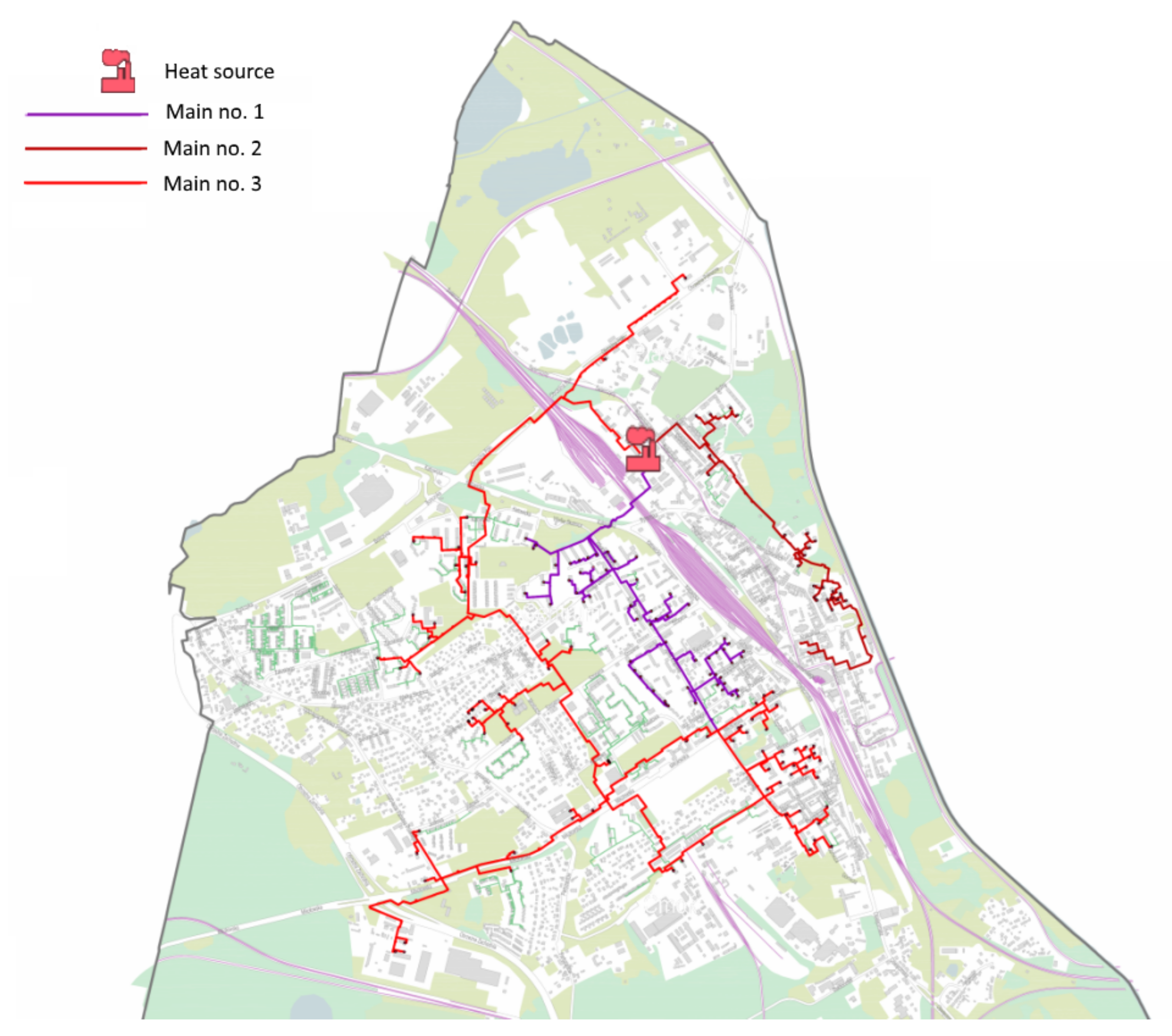
The heating market of the analyzed city can be divided into two zones: a downtown area (selected for analysis) and a suburban area. The downtown is an insular/separated market supplied by one heating plant, and there is the lack of an emergency/reserve heat source. The heating plant is practically located in the city center, and the district heating network consists of three mains (Figure 2).

General information about size and heat demand in the analyzed network:

• Total sales: approx. 60 MW (out of which, 7 MW is used for domestic hot water), or about 340 thousand GJ per year
  • Main No. 1—68 heat sale nodes—10 MW;
  • Main No. 2—24 heat sale nodes—8 MW;
  • Main No. 3—401 heat sale nodes—42 MW.
• Customers:
  • Residential buildings;
  • Public institution buildings (educational, health, cultural);
  • Detached houses.

According to the theory and construction practice of such tools, through the mathematical representation of its elements and the relationships between the real system and its implementation in the modelling system, the model makes it possible to calculate the decision variables based on scenario assumptions. In particular, the main outcomes from the model were as follows:

• The optimal level of thermal power generation (purchase) in heating plant;
• The optimal level of heat production (purchase);
• The flow rate of the heating medium in the heat source, nodes, and edges of the network;
• The average daily temperature of the heating medium in the heat source, nodes, and edges of the network;
• The average daily pressure of the heating medium in the heat source, nodes, and edges of the network;
• The heat, power, and temperature losses in each edge of the analyzed network;
• The disposable pressure and pressure losses in each edge of the analyzed network;
• The costs of heat purchase and heat transmission—minimization;
• The electricity costs associated with the operation of the pumps in the network.

5. Results and Discussion

The final model consisted of 244 nodes and 241 edges. The calculations were carried out in a loop set for 365 days—examining the thermal and pressure modules. The flow module was solved twice—for the winter and the summer period. The model statistics, along with the solving time for all three modules for one day, are shown in

Table 1. Model statistics.

Parameter	Flow	Thermal	Pressure	Total
	Module	Module	Module
Number of variables	1105	2739	1651	5495
Number of equations	1105	3789	4442	9336
Number of non-zero elements	2745	8310	6154	17,209
Solving time for 1 day—CPLEX [sec]	—	—	—	8.3
Solving time for 1 day—GUROBI [sec]	—	—	—	8.8
Solving time for 365 days—CPLEX [sec]	—	—	—	36.2
Solving time for 365 days—GUROBI [sec]	—	—	—	36.7

.

The total computation time using the CPLEX server was 8.3 s, while it was 8.8 s using the GUROBI server (for 1 day), and it was 36.2 s for CPLEX and 36.7 s for GUROBI (for 365 days). The results indicate that the calculation time using the GUROBI solver was a little longer, which led to the fact that it could be used for calculations; however, the use of the CPLEX solver is recommended. It is also possible to use various types of solvers used to solve linear problems. The calculation time for both solvers shows that the model can be easily used for the design and development of district heating networks. The obtained result is satisfactory from the point of view of making management decisions in the area of district heating network management.

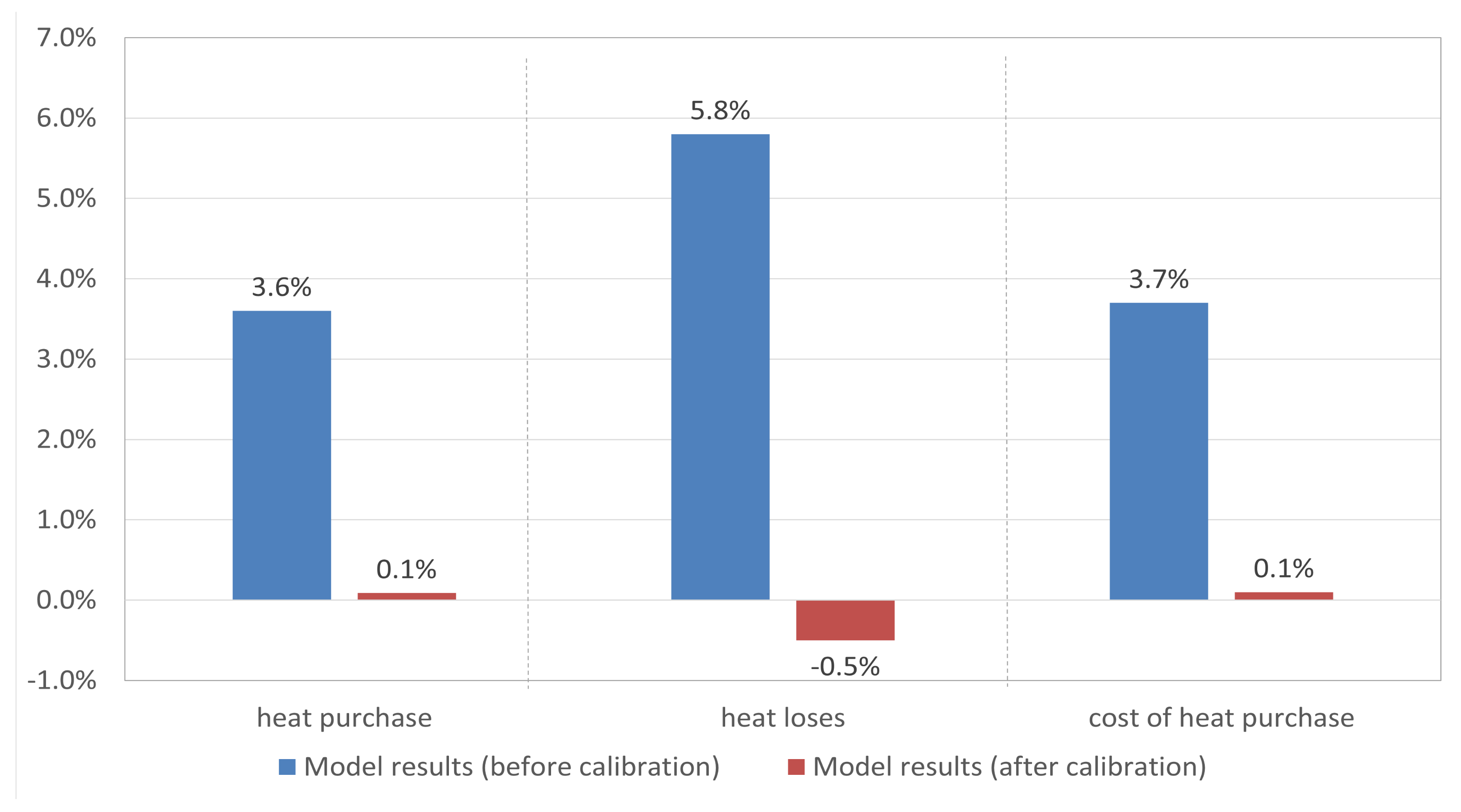
The model was calibrated using historical data obtained from the owner of the district heating network. Before calibration, the difference in calculated values of heat purchase compared to historical values was 3.6% (annual). Due to the differences in the process of obtaining and aggregating information on the consumption and settlement of heat sales in individual sections of the network, there were differences in the values of heat sales/transmission losses in individual periods of the year (winter season/summer season) in the model. We noticed that, in winter periods, the values indicated by the model vs. historical values were slightly underestimated, while, in the summer season, they were overstated. As a consequence, we performed additional calculations by introducing calibration factors (which were different for the winter season and different for the summer season). The determination of the calibration coefficients was carried out in steps of 1%. Finally, for the tested section of the network (constituting the case study), the value of the correction factor for the winter season was +7%, while, for the summer season, it was −15%. As a consequence, the results of the model, after the calibration process, were very similar to the real data (all percentage deviations were within 1%).

The results of the model, after the calibration process, were very similar to the real data (all percentage deviations were within 1%). Figure 3 presents the accuracy outcomes of the following variables: heat purchase, heat losses, and total cost of heat purchase.

Due to data confidentiality, we cannot provide detailed calculation results. However, we can present details about the selected edge. The temperatures in the supply network and the return network for an arbitrary edge are shown in (Figure 4). In the period from day 139 to 265, the flow temperature was at the lower limit (70 ${}^{°}$C); on days 1–99 and 322–365, there were large changes between days. For the rest (99–139 and 265–322), the temperature remained at an almost constant level (about 73.4 ${}^{°}$C) above the lower limit. The temperature in the return network varied from 43 ${}^{°}$C to 60 ${}^{°}$C. Note as well that the temperature in the supply network did not reach the assumed maximum (140 ${}^{°}$C), nor did it reach the assumed minimum in the return network (40 ${}^{°}$C).

The pressure in an arbitrarily selected edge is shown in Figure 5. The pressure in the supply network was 610–670 kPa in the winter season (days 1–138 and 266–365), and, in the summer season (days 138–265), it was at the level of 394–423 kPa. In the return network, the pressure was constant and amounted to 250 kPa in the summer season and 286 kPa in the winter season.

The model provided such values for each node and edge in the supply and return network, as well as values for temperature, pressure losses, and other relevant network parameters. For example, one can estimate the cost of heat loss by month (see Figure 6).

6. Conclusions

The proposed tool can be used in the design of a new heating network or in the extension of an existing one. Thanks to the ability to accurately model important physical conditions in the entire network and in each of its elements, it was possible to check the correctness of its operation for various weather conditions, to select operating points, and to check the profitability of the investment. The size of the example is quite large, and the current computing capabilities do not exclude testing the model for more extensive networks, which may be the subject of further publications.

The article has shown how to construct a decision-supporting tool which can be utilized in the context of investment decisions for district heating companies operating in a specific location. The developed decision support system for a district heating system meets the requirements formulated in Section 3.1. The mathematical model was composed of three modules, namely (i) a flow model, (ii) a thermal model, and (iii) a pressure model; decomposition was applied to deal with non-linear dependencies. The tool was implemented in GAMS (general algebraic modeling system), which is a high level modeling platform, and the calculations were obtained using CPLEX solver. The difference between historical data were within 1%, which revealed the high level of accuracy of the computation.