Non-Intrusive Load Decomposition Based on Instance-Batch Normalization Networks

Abstract

At present, the non-intrusive load decomposition method for low-frequency sampling data is as yet insufficient within the context of generalization performance, failing to meet the decomposition accuracy requirements when applied to novel scenarios. To address this issue, a non-intrusive load decomposition method based on instance-batch normalization network is proposed. This method uses an encoder-decoder structure with attention mechanism, in which skip connections are introduced at the corresponding layers of the encoder and decoder. In this way, the decoder can reconstruct a more accurate power sequence of the target. The proposed model was tested on two public datasets, REDD and UKDALE, and the performance was compared with mainstream algorithms. The results show that the F1 score was higher by an average of 18.4 when compared with mainstream algorithms. Additionally, the mean absolute error reduced by an average of 25%, and the root mean square error was reduced by an average of 22%.

1. Introduction

Non-intrusive load monitoring (NILM) technology decomposes the total load information at a power entrance to obtain information about the amount of electricity consumption of each equipment load, providing technical support for efficient power management [1,2]. NILM technology is a low-cost energy consumption monitoring and management method that can effectively reduce energy waste in buildings and has important practical implications for achieving “carbon peaking” and “carbon neutrality” [3,4].

NILM was first proposed by Professor George W. Hart in 1992 and was developed to simplify the process of collecting energy consumption data [5]. The development of instrumentation, computer technology, and the release of various public datasets such as REDD [6] and UK-DALE [7], provided a database and technical support system for non-invasive load decomposition [2]. Kelly et al. developed a non-invasive load decomposition toolkit (NILMTK) based on traditional algorithms in 2014 [8]. Then, they started investigating the application of deep learning algorithms in this field and used long short-term memory (LSTM) networks, denoising autoencoders (DAE), and convolutional neural networks (CNN) to solve non-intrusive load decomposition problems in 2015 [9]. In 2019, Batra et al. updated the toolkit by including the latest algorithms capable of performing load decomposition tasks at that time [10].

Up until now, the vast amount of NILM research that has been conducted by domestic and foreign scholars can be divided into two categories based on the frequency of data acquisition: (1) load decomposition methods based on high-frequency data and (2) load decomposition methods based on low-frequency data [2]. The data acquired by high-frequency acquisition (>1 Hz) contain richer information in regard to certain electrical parameters, such as harmonics, electromagnetic interference, V-I trajectory information, etc. For example, reference [1] collects harmonics, voltage-to-ampere ratio coefficients, and other features from real data, and proposes a non-intrusive load identification method based on the feature-weighted k-nearest neighbor (KNN) algorithm, solving the problem of misjudgment when identifying certain classes of loads in unbalanced datasets. In prior research [3], there have been instances of U-I trajectory images being constructed using voltage and current data acquired at high frequencies, while devices are accurately identified using a non-intrusive load decomposition method based on color coding. However, the acquisition of high-frequency data requires high-level measurement equipment, which involves a complex process of high costs and is therefore not suitable for residential electricity loads [11].

For these reasons, researchers have shifted their focus to the study of improving the accuracy of load decomposition based on low-frequency data (≤1 Hz) obtained from smart meters [12]. Prior work [13] proposed the adaptive density peak clustering-factorial hidden Markov model (ADP-FHMM) to reduce the dependence of prior information. Another study [14] introduced the appliances ON-OFF state identification factor in the hidden Markov model (HMM) to improve the accuracy of load decomposition. In [15], a non-linear support vector machine (SVM) approach is proposed to address the NILM problem. The method uses power differences to detect events for the switching states of electrical equipment, and [16] used the K-nearest neighbor algorithm (KNN) to solve the NILM problem, investigating the optimal settings of KNN variants.

However, both HMM-based methods and machine learning methods, such as SVM and KNN-based methods, require manual feature extraction. In contrast, deep neural network methods can automatically extract features without human involvement [17]. Prior work [18] has used the convolutional neural nets (CNN) model with sequence to point (seq2point) to reduce the misclassification rate of load decomposition. In another study [19], a preliminary exploration of the appliance transfer learning (ATL) and cross region transfer learning (CTL) capabilities of the model proposed in reference [18] was conducted, and the experimental results demonstrated that, while the seq2point model displays some capacity for generalization performance, parameter tuning is still required when applied to different datasets. Others [11] improved on this algorithm [18] by introducing the channel attention and spatial attention mechanisms into the sequence-to-point model, which improved the load decomposition efficiency. Another study [20] proposed a load disaggregation with attention (LDwA) model, which combines a regression sub-network with a classification sub-network. Here, the regression sub-network uses an encoder-decoder structure with an attention mechanism, and the classification sub-network uses a full convolutional network, relatively improving the generalization ability of the model. However, there is no evidence of any improvement with regard to the decomposition effect for multi-state appliances.

Although the performance of non-intrusive load decomposition methods for low-frequency sampling has greatly improved, generalization performance remains a comparatively difficult challenge to overcome. Therefore, in this paper, we seek to improve upon the classical seq2point model by applying instance-batch normalization networks (IBN-Net) to achieve better generalization performance capabilities in the field of non-intrusive load decomposition. The proposed model uses an encoder-decoder structure with a fused attention mechanism, in which the encoder and decoder are composed of multiple layers of IBN-Net with integrated instance normalization (IN) and batch normalization (BN) structures. This model allows the shallow output of the encoder to be fed into the corresponding layer of the decoder using a skip connection, improving the multi-scale information fusion capability of the network, and helping the encoder to construct more accurate power sequences of the target appliances. In this paper, the model is trained and tested using two publicly available datasets, REDD and UK-DALE. We also compare the proposed algorithm with current, more advanced algorithms, and the experimental results provide support for the accuracy and effectiveness of our proposed algorithm.

2. Non-Intrusive Load Decomposition Model

2.1. Non-Intrusive Load Decomposition Problem Modeling

The purpose of non-intrusive load decomposition is to obtain the power information of individual power-using devices by collecting the total load power information at the power inlet via the energy decomposition method. The only power information required by the proposed algorithm is the active power data that can be sampled at low frequencies. The decomposition task model can be described as follows: the total power sequence of a household within a period of time $T$ is $Y$, where $Y=\left\{y_1,y_2,\cdots ,y_T\right\}$, and each element within the sequence $y_t$ is the sum of the power of all power-using devices in the household at the time of $t$; and assuming that the household has M devices, the power sequence of the $i$ device at the corresponding time can be expressed as $X_i$, where $X_i=\left\{x_{i1},x_{i2},\cdots ,x_{iT}\right\}$, and $x_{it}$ represents the power of the $t$ device at the time of $i$. The model can then be expressed as follows:

$${\mathrm{y}}_t={\displaystyle \sum _{i=1}^M{x}_{it}}+ϵ$$

(1)

where $ϵ$ is a Gaussian noise factor with zero mean. The principle of non-intrusive load decomposition is to use the total power measurements to estimate the power values of individual devices.

2.2. Seq2point Framework

In recent years, the seq2point model and its variants have been widely used in the field of load decomposition; these predict the corresponding window sequence midpoint values of individual equipment loads from a fixed-length sequence of total load windows [11]. The load decomposition model of the seq2point architecture can be expressed as

$$x_{\tau }=F_b\left(Y_{t:t+L-1}\right)+ϵ$$

(2)

where the input to the model is $Y_{t:t+L-1}$, which is a sequence of total power windows with a window length of $L$; the output is the midpoint element of the corresponding sequence of target appliance windows $x_{\tau }$, where $\tau =t+\left[L/2\right]$. $F_b$ is the neural network that maps the input $Y_{t:t+L-1}$ to the output and $x_{\tau }$; and $ϵ$ is the $L$ dimensional Gaussian noise. Before processing the input power sequence, it is necessary to complete the first and last ends of the complete input power sequence with $L/2$ zero elements [18]. The method described in the paper uses a sequence-to-point mapping approach, which avoids interference from edge information of window sequences and improves the model’s generalization performance.

2.3. Flow Chart of Load Decomposition in This Paper

Figure 1 shows the flow of non-intrusive load decomposition in this study. It is easy to see from the flow chart that this study utilizes specific models for each individual appliance, while the network structure is constructed according to: (1) the physical meaning of non-intrusive load decomposition, and (2) the balance between the related strengths and weaknesses of each sub-network for the encoding and decoding processes. This approach avoids the potential network redundancy caused by the simple splicing of deep learning network structures.

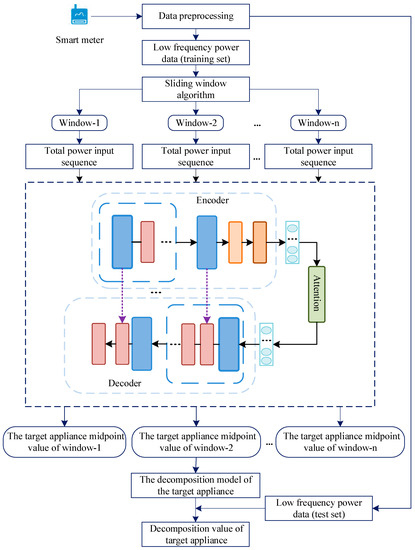
Figure 1. Flow chart of load decomposition in this study.

3. Seq2point Model Based on IBN-Net Codec Mechanism

In this paper, a sequence-to-point architecture is used, with internal replacement serving as an IBN-Net-based encoding-decoding mechanism, while the whole network consists two components, as shown in Figure 2. The encoder extracts the power information of the target appliance from the total power window sequence $Y_{t:t+L-1}$ and maps it to the context vector $C$, $C=\{h_1,h_2,\dots ,h_L\}$, $h_t$ for the hidden state at the moment of the input sequence $t$ generated during the encoding process. This is represented by Equation (3).

$$C=f_e\left(W{Y}_{t:t+L-1}+b\right)$$

(3)

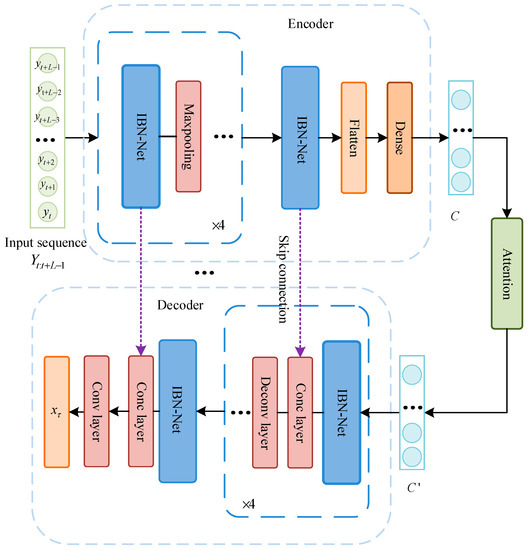
Figure 2. Model structure diagram.

The decoding process is shown by Equation (4):

$$x_{\tau }=f_d\left(W^{\prime }{C}^{\prime }+b^{\prime }\right)$$

(4)

where: $f_e$ is the encoding function; $f_d$ is the decoding function; $W$, $b$ and $W^{\prime }$, $b^{\prime }$ are the function weights and biases of the encoding and decoding layers, respectively; and $C^{\prime }$ is the dynamically variable context vector in the decoding process, which is generated by the attention mechanism between the encoder and decoder.

The encoder primarily consists multiple IBN-Net sub-modules, each of which is followed by a maximum pooling layer to reduce the temporal resolution and facilitate the network learning the high-level features of the target device, while the output of the IBN-Net stack is converted into a context vector C by a fully connected layer (Dense). The decoder has a similar structure to the encoder, consisting the same number of IBN-Net modules, where each IBN-Net is followed by a deconvolution layer to progressively increase the temporal resolution and reconstruct the signal from the target device. In addition, a skip connection function has been added to connect the output of the corresponding IBN-Net layer from the encoder to the decoder, as shown in Figure 2. The skip connection can help the decoder better fuse the features extracted from the shallow network of the encoder and allow for a more accurate reconstruction of the target device power sequence. Skip connections between corresponding layers in the encoder and decoder are implemented using the concatenate (Conc) layer. After repeated experiments, the number of layers of the IBN-Net sub-module in the encoder was determined to be five layers. The maximum pooling layer divides the temporal resolution by two for each step in the encoder, while the deconvolution operation in the decoder multiplies the temporal resolution in the decoder by two.

3.1. IBN-Net Sub-Module

The instance and batch normalization network is a new convolutional network structure that integrates instance normalization (IN) and batch normalization (BN) [21,22]. This integration enhances the CNN’s generalization ability across domains (e.g., load data of other households or other datasets) without fine-tuning [23].

Depending on the different configurations of BN and IN, the IBN-Net can have different structures and be applied to a variety of scenarios. The structure of the IBN-Net sub-module in this paper is shown in Figure 3. The IBN-Net consists three consecutive convolutional layers with a shallow convolutional module combining batch normalization and a corrected linear unit activation function (ReLU). The number of filters in the convolutional layers in all IBN-Net networks is either 64 or 256, respectively, and the kernel size is three. The input of the IBN-Net is connected to the instance normalization layer using residual connections so that the gradients can circulate throughout the model during training, effectively preventing the gradient disappearance problem.

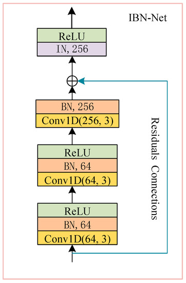
Figure 3. IBN-Net structure diagram.

3.2. Attention Mechanism

In the classical encoder-decoder architecture, only the context vector $C$ is used between the codecs to represent the information of the whole input sequence. As a result, the fixed-length vector $C$ is not capable of carrying all the information from the input when the length of the input sequence increases to a certain level, revealing the limitations of the model’s information processing capabilities. The introduction of the attention mechanism solves this problem by providing the model with a corresponding focus that can be enabled at different points during decoding, thus enhancing the information utilization capability of the model [24].

Inspired by a previous study [18], the attention mechanism between the encoder and the decoder in this study was designed as a single-layer feedforward neural network. This neural network computes the attention weights and returns a weighted average of the encoder’s output over time, i.e., the context vector $C^{\prime }$. The attention unit captures moments of significant activation by the target device in the encoder output features, extracting the feature information that is deemed to be most valuable for decomposition. This process allows the network to implicitly detect certain events (e.g., turning devices on or off) and specific signal components (e.g., high power consumption) for the purpose of assigning them higher weights. The calculation process of the attention unit is shown in Figure 4. Its mathematical definition is shown in Equations (5)–(7).

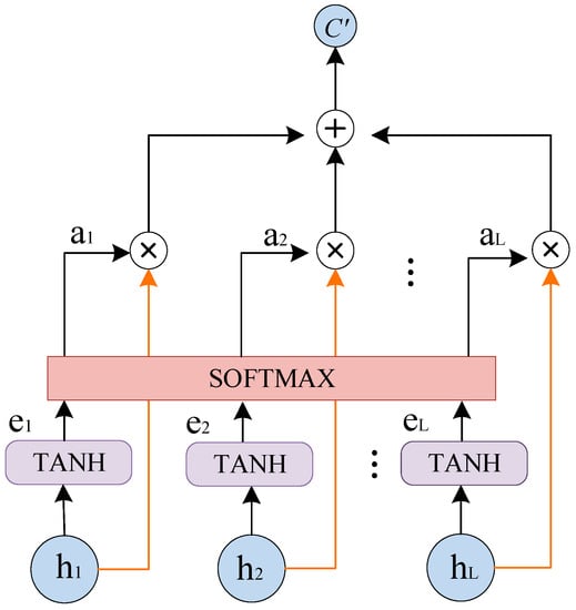
Figure 4. Structure of attention mechanism.

Its mathematical definition is

$$e_t=V_a{}^{\mathrm{T}}\times \tanh (W_a{h}_t+b_a),t=1,2,\cdots ,L$$

(5)

$${\alpha }_t=\frac{\exp (e_t)}{{\displaystyle \sum _{j=1}^L\exp (e_{\mathrm{j}})}},t=1,2,\cdots ,L$$

(6)

$$C^{\prime }={\displaystyle \sum _{t=1}^L{\alpha }_t}{h}_t$$

(7)

where $V_a$, $W_a$, and $b_a$ are parameters learned in conjunction with other components of the network and are continuously adjusted with training.

4. Data Pre-Processing and Experimental Setup

4.1. Dataset Selection

The following two publicly available datasets, which contain data from different countries, were selected for this paper.

The UK-DALE dataset [6] was first published by Jack Kelly in 2015 and contains data on the active power (as distinguished from total power) and sub-devices of five UK homes. The five houses that were analyzed contain 54, 20, 5, 6, and 26 sub-metering devices, respectively, with a sampling period of 6 s collected over roughly 1 to 2.5 years.

The REDD dataset [7] was released in 2011 and collected data on the total house power and sub-equipment energy consumption from six U.S. households, sampled at 1 Hz. It also contains high-frequency data on the main power supply of the two houses, though it should be noted that the model in our study is primarily concerned with energy consumption data sampled at low frequencies.

4.2. Electrical Selection

Regarding appliance selection, four appliances were selected for this paper: a refrigerator, a dishwasher, a microwave oven, and a washing machine. These four appliances were chosen in accordance with the findings of prior research, while also considering the distribution of appliances in the two aforementioned datasets. Additionally, the different operating characteristics of the four appliances allow for a full verification of the proposed model’s load decomposition performance. Refrigerators (RF) and microwaves (MW) are typical switching appliances, while washing machines (WM) and dishwashers (DW) are multi-state appliances. They exist in multiple households in both datasets, which is beneficial when testing for generalization performance.

4.3. Data Pre-Processing

Since the sampling frequencies of the two datasets are not uniform, it was necessary to downsample the REDD dataset; this downsampling was performed using a 6 s sampling interval.

After downsampling, missing data were patched and missing data longer than 3 min (i.e., those with more than 30 consecutive missing data points) were attributed to device shutdown; therefore, the corresponding elements were nullified. Gap filtering was performed for data segments that were missing data shorter than 3 min (i.e., those with less than 30 consecutive missing data points). The gap filtering was performed according to previously established methods [25].

After obtaining the experimental data, the data were normalized using Equation (8).

$$z=\frac{z_t-z_p}{\sigma }$$

(8)

where $z$ is the normalized value; $z_t$ indicates the reading of the total power supply or experimental appliance at time t; $z_p$ indicates the mean value of the total power supply or experimental appliance, and $\sigma$ indicates the standard deviation of the total power supply or of the experimental appliance. The mean and standard deviation were calculated from the data used in the current experiment.

4.4. Experimental Setup

The hardware environment uses a 64-bit computer with an Intel(R) CoreTM i7-11700 CPU @ 2.5 GHz and a GeForce GTX3060. The software platform is a Win10 operating system running Python 3.6.13 (64-bit) and the Tensorflow 2.4.0 framework. The development environment of the experiment was created using the NILMTK v0.4. Keras, an artificial neural network library using TensorFlow as its backend, was used to build the model in this study. The mean square error was chosen as the loss function and the Adam optimizer was used to adjust the model parameters. The validation set loss during training was monitored using the ModelCheckpoint callback function in Keras for the purpose of saving the best models that emerged during the training process. All experiments were iterated for 100 epochs, and early stopping was used during the training process to prevent overfitting. The patience of the early stopping mechanism was set to 20, i.e., we waited for 20 epochs following the last validation loss improvement before interrupting the training loop.

Figure 5 shows the trend of validation loss and training loss during one of the training sessions. The yellow curve represents the validation loss, and the blue curve represents the training loss. The horizontal axis indicates the number of training iterations, and the vertical axis represents the value of loss. During the training process, the validation loss reached its minimum value at the 67th iteration, at which point the weights and other training parameters were saved. The validation loss did not decrease further during the next 20 iterations, so the training loop was interrupted at the 87th iteration, according to the early stopping mechanism. It is worth noting that both the “train_loss” and “val_loss” are dimensionless values because they were normalized during the data pre-processing stage.

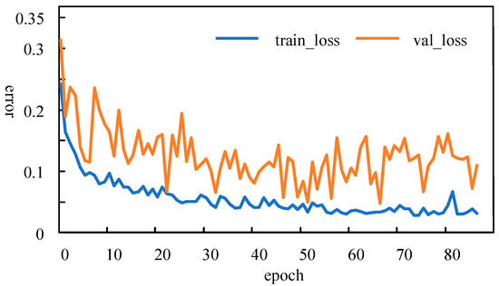
Figure 5. Graph of the trend of loss for a particular training session.

4.5. Performance Metrics

Mean absolute error (MAE) and root mean square error (RMSE) are commonly used in the field of non-invasive load decomposition as metrics to evaluate the decomposition accuracy of algorithms [2]. Therefore, this study likewise used these two kinds of performance metrics to analyze the load decomposition accuracy. The calculation methods are shown in Equations (9) and (10), respectively.

$$MAE=\frac{1}{m}{\displaystyle \sum _{k=1}^m|x_k^{\prime }-x_k|}$$

(9)

$$RMSE=\sqrt{\frac{1}{m}{{\displaystyle \sum _{k=1}^m\left(x_k^{\prime }-x_k\right)}}^2}$$

(10)

where m is the number of sample points; $x_k$ is the true value of the kth sample point of the target appliance; and $x_k^{\prime }$ is the predicted value of the k-th sample point of the target appliance. Both MAE and RMSE are expressed in watts.

In addition, to measure the recognition accuracy of each device being in either the on or off state, we used the classification metric F1 score, which is the harmonic mean of precision (P) and recall (R).

$$F1=\frac{2P\cdot R}{P+R}$$

(11)

$$P=\frac{TP}{TP+FP}$$

(12)

$$R=\frac{TP}{TP+FN}$$

(13)

where TP indicates the number of samples when the target appliance is actually in operation and the predicted value is determined to be in operation; FP indicates the number of samples when the target appliance is actually off and the predicted value is determined to be in operation; and FN indicates the number of samples when the target appliance is actually in operation and the predicted value is determined to be off [20]. When the active power is greater than a specific threshold, the appliance is considered to be “on”, and when the active power is less than or equal to the same threshold, it is considered to be “off.” The particular threshold, 15 W, was chosen in accordance with prior studies [20]. Precision, recall, and the F1 score were represented by a value between 0 and 1. A higher F1 score indicates a better classification performance for the model [12].

5. Discussion

In order to verify the decomposition ability and generalization of the method in this paper, the same experimental appliances were trained and tested within the same house, as well as within different houses in the UK-DALE dataset. The proposed method was also compared and analyzed against the more advanced DAE [9], Seq2seq [18], Seq2point [18], and LDwA [20] algorithms. The evaluation metrics obtained from the experiments were retained to three decimal places.

5.1. Comparison and Analysis of Experimental Results of the Same House

In the same house experiment, four kinds of experimental appliances—refrigerator, microwave, washing machine, and dishwasher—were trained and tested using low-frequency power data from house 1. Different time periods were selected for the training and testing sets, and there was no intersection between them. The results of the performance metrics for this experiment are shown in Table 1. The last column of Table 1 is the average value of the performance metrics of the four types of electrical appliances obtained by each algorithm in the experimental results. “IBN-Net” in Table 1 denotes the model proposed in the paper.

Table 1. Comparison of experimental results of several algorithms.

Metric	Models	RF	WM	DW	MW	Average
MAE (W)	DAE	24.071	23.352	13.631	13.376	18.608
	Seq2seq	23.441	15.315	8.794	9.725	14.319
	Seq2point	20.169	18.967	8.759	11.659	14.889
	LDwA	19.037	13.416	8.954	8.694	12.525
	IBN-Net	15.855	9.707	7.057	8.192	10.203
RMSE (W)	DAE	37.578	141.003	119.317	86.412	96.078
	Seq2seq	34.437	117.376	95.186	73.740	80.185
	Seq2point	34.665	118.916	88.592	83.978	90.788
	LDwA	29.154	85.112	66.712	76.037	64.254
	IBN-Net	28.529	75.163	59.491	71.365	58.637
F1	DAE	0.783	0.253	0.332	0.313	0.420
	Seq2seq	0.792	0.533	0.608	0.454	0.597
	Seq2point	0.832	0.664	0.646	0.480	0.656
	LDwA	0.905	0.822	0.672	0.689	0.772
	IBN-Net	0.916	0.871	0.753	0.819	0.840

From the results of the evaluation metrics in Table 1, it can be seen that the error and F1 scores of Seq2point and LDwA place them in a better position among the algorithms compared, but both are inferior to the algorithm proposed in this study. In terms of average values, when compared with the Seq2point and LDwA algorithms, our model shows a reduction in the RSME by 35.4% and 8.7%, while the MAE is reduced by 31.5% and 18.5%, and the F1 scores are improved by 28% and 8.8%, respectively. Among them, the reduction of error indicators for the dishwasher and washing machine is larger; the RMSE is reduced by 10% and 11.7%, and the MAE is reduced by 21% and 27.6%, respectively. It demonstrates that the model proposed in this study greatly improves the load decomposition capabilities of multi-state appliances. Preliminary analysis concludes that this is due to the introduction of the skip connection, which is further supported by the ablation experiment in Section 4.4. In summary, the model proposed in this study displays a higher load decomposition accuracy for low-frequency sampling data.

Figure 6 shows results from the same house experiment, and the graphs show the comparison curves of the four kinds of experimental appliances’ real power usage along with the power usage predicted by the proposed model. According to the fitting degree and tracking effect shown in the figure, it can be concluded that the power decomposition results of the proposed model are close to the real power usage.

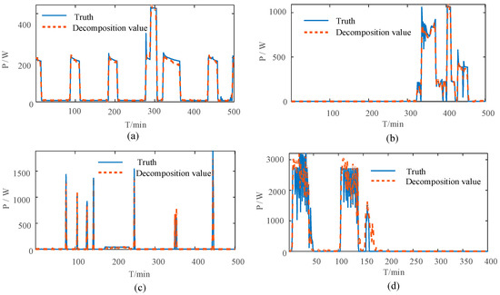
Figure 6. Example graph of experimental results of the same house (a) Refrigerator (b) Dishwasher (c) Microwave (d) Washing machine.

5.2. Comparison and Analysis of Experimental Results of Different Houses

In the practical application of NILM, trained models are mostly applied to unknown families; therefore, the generalization performance of a model is especially important. To assess this aspect, experiments were conducted using different room data from the UK-DALE dataset for training and testing, respectively, with the training set coming from Households 1 and 2 and the test set coming from Household 5. The Seq2point and the LDwA model, with a high accuracy of load decomposition in the experiments of the previous section, were chosen to compare the generalization performance with the model proposed in this paper. The experimental results of different houses are shown in Figure 7, which shows the average values of the four experimental appliance evaluation metrics.

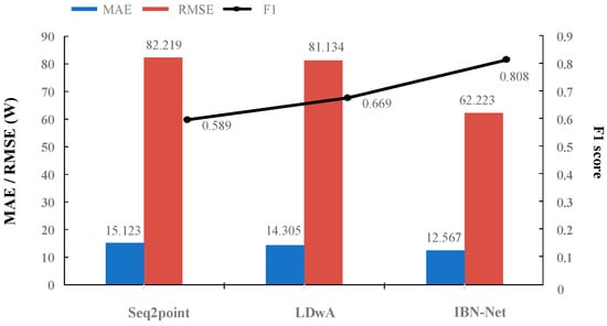
Figure 7. Comparison of the results of several algorithms for different house experiments.

According to the results in Figure 7, it can be seen that the decomposition accuracy of our proposed model is higher when the experiments are conducted in different houses. This indicates that the generalization performance of our model is better than that of the two comparison models.

5.3. Comparison and Analysis of Experimental Results of Transfer Learning

Considering the comprehensiveness of the evaluation, the cross-region transfer learning capability (CTL) of the model was verified. The UK-DALE dataset was selected as the training set and the REDD dataset was selected as the test set. The experimental results are shown in Figure 8, where the evaluation metrics are taken as an average of the four experimental appliances. From Figure 8, it can be seen that, compared with the seq2point and LDwA models, the model proposed in this study has fewer errors and higher F1 scores. That is, the proposed model exhibits a better cross-region transfer learning ability while still maintaining accuracy when applied to unknown rooms in different regions. The experimental results of CTL have achieved the desired objectives and verify the validity of the model.

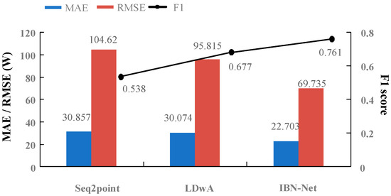
Figure 8. Comparison of CTL experimental results.

5.4. Ablation Experiment

To verify the effectiveness of the network, we conducted ablation experiments for family 1 in the UK-DALE dataset, and verified the effectiveness of the attention mechanism, instance and batch normalization, and skip connection. The model’s performance was further improved by setting up three different codec model construction schemes and quantitatively evaluating the performance of the different modules. The experimental results are shown in Table 2. Scheme A involves replacing the IBN-Net subnetwork of the model depicted in Figure 2 with CNN and removing the skip connections. Scheme B builds upon Scheme A by adding skip connections between corresponding layers in the encoder and decoder. Scheme C refers to the removal of the attention module from the model shown in Figure 2. This is done to perform an ablation analysis of the attention mechanism and to investigate its contribution to the performance of the model. Compared with the other three schemes, our model performed better based on both evaluation metrics. In terms of average values, the F1 score of Scheme B was reduced by about 6% and the MAE increased by about 34% compared with our proposed method. Comparing with Scheme B, it was found that the F1 score of Scheme A was reduced by about 7% and the MAE of Scheme A increased by about 16%, indicating that the skip connection had a positive effect on the performance of the model. Comparing Scheme C with our method, it can be observed that the F1 score is reduced by 3% and the MAE is increased by 12%. These results show that the attention mechanism, instance and batch normalization, and the skip connection have an enhancing effect on network performance.

Table 2. Comparison of results of ablation experiments.

Metric	Model Solutions	IN and BN	Skip Connection	Attention	RF	WM	DW	MW	Average
MAE (W)	A			√	21.243	13.445	9.386	10.538	13.653
	B		√	√	24.005	15.865	11.175	12.263	15.827
	C	√	√		17.758	10.874	7.907	9.170	11.427
	Complete model	√	√	√	15.855	9.707	7.057	8.192	10.203
F1	A			√	0.817	0.744	0.643	0.732	0.734
	B		√	√	0.861	0.818	0.707	0.770	0.789
	C	√	√		0.887	0.845	0.732	0.798	0.815
	Complete model	√	√	√	0.916	0.871	0.753	0.819	0.840

It is worth noting that the ablation of the skip connection has a more significant impact on the experimental results for washing machines and dishwashers. In the configuration without the skip connection (Scheme A), the F1 score for these appliances was reduced by about 9% and the MAE increased by about 20% compared with the skip connection (Scheme B) configuration. This indicates that when the skip connection is used to fuse the features extracted from the encoder layer to the corresponding decoder layer, the ability to identify multi-state devices is improved. The results of the ablation experiments are consistent with the previous analysis. It suggests that the inclusion of attention mechanism, skip connection, and application of IN and BN can enhance the performance of the model for decomposition in this particular study.

6. Conclusions

In this paper, we proposed a non-invasive load decomposition method based on an attention mechanism and a sequence translation model. The model consists mainly multilayer IBN-Net subnetworks in the encoder and decoder. The batch normalization (BN) module in the subnetwork enhances the network’s ability to discriminate features and facilitates the encoder’s ability to map more relevant features to the hidden layer, while the shallow instance normalization (IN) module in the subnetwork improves the generalization performance of the network. The skip connection between the encoder and decoder transmits the features extracted from the IBN-Net in the encoder directly to the corresponding IBN-Net layer in the decoder, enabling the decoder to reconstruct a more accurate power sequence of the target appliance. The usefulness of the skip connection is especially obvious when targeting multi-state appliances. In addition, the attention mechanism between the encoder and decoder can help the decoder generate more accurate appliance activation by changing the context vector. The proposed model was compared with state-of-the-art NILM methods using the UK-DALE and REDD data sets, and significant results were obtained. Compared with current, more advanced algorithms, our model increases the F1 score by 18.4% on average, while decreasing the MAE by an average of 25% and the RMSE by an average of 22%.

References

- Zhu, H.; Cao, N.; Deer, H.; Zhang, Z.; Ke, W. Non-intrusive load identification method based on feature-weighted KNN. Electron. Meas. Technol. 2022, 45, 70–75. [Google Scholar]
- Deng, X.P.; Zhang, G.Q.; Wei, Q.L.; Wei, P.; Li, C.-D. A survey on the non-intrusive load monitoring. Acta Autom. Sin. 2022, 48, 644–663. [Google Scholar]
- Cui, H.Y.; Cai, J.; Chen, L.; Jiang, C.; Jiang, Y.; Zhang, X. Non-intrusive load fine-grained identification based on color encoding. Power Syst. Technol. 2022, 46, 1557–1565. [Google Scholar]
- Chen, J.; Wang, X.; Zhang, H. Non-intrusive load recognition using color encoding in edge computing. Chin. J. Sci. Instrum. 2020, 41, 12–19. [Google Scholar]
- Hart, G.W. Nonintrusive appliance load monitoring. Proc. IEEE 1992, 80, 1870–1891. [Google Scholar] [CrossRef]
- Kolter, J.Z.; Johnson, M.J. REDD: A public data set for energy disaggregation research. In Proceedings of the Workshop on Data Mining Applications in Sustainability (SIGKDD), San Diego, CA, USA, 21 August 2011; Volume 25, pp. 59–62. [Google Scholar]
- Kelly, J.; Knottenbelt, W. The UK-DALE dataset, domestic appliance-level electricity demand and whole-house demand from five UK homes. Sci. Data 2015, 2, 150007. [Google Scholar] [CrossRef]
- Batra, N.; Kelly, J.; Parson, O.; Dutta, H.; Knottenbelt, W.; Rogers, A.; Singh, A.; Srivastava, M. NILMTK: An Open Source Toolkit for Non-intrusive Load Monitoring. In Proceedings of the 5th International Conference on Future Energy Systems (ACM e-Energy), Cambridge, UK, 11–13 June 2014; pp. 265–276. [Google Scholar]
- Kelly, J.; Knottenbelt, W. Neural NILM: Deep Neural Networks Applied to Energy Disaggregation. In Proceedings of the 2nd ACM International Conference on Embedded Systems for Energy-Efficient Built Environments, Seoul, Republic of Korea, 4–5 November 2015; pp. 55–64. [Google Scholar]
- Batra, N.; Kukunuri, R.; Pandey, A.; Malakar, R.; Kumar, R.; Krystalakos, O.; Zhong, M.; Meira, P.; Parson, O. A demonstration of reproducible state-of-the-art energy disaggregation using NILMTK. In Proceedings of the 6th ACM International Conference, New York, NY, USA, 13–14 November 2019; pp. 358–359. [Google Scholar]
- Xu, X.; Zhao, S.; Cui, K. Non-intrusive load disaggregate algorithm based on convolutional block attention module. Power Syst. Technol. 2021, 45, 3700–3705. [Google Scholar]
- Liu, R. Non-Intrusive Load Decomposition Based on Data Augmentation and Deep Learning; Zhejiang University: Hangzhou, China, 2021. [Google Scholar]
- Wu, Z.; Wang, C.; Peng, W.; Liu, W.; Zhang, H. Non-intrusive load monitoring using factorial hidden markov model based on adaptive density peak clustering. Energy Build. 2021, 244, 111025. [Google Scholar] [CrossRef]
- Yu, C.; Qin, Z.J.; Yang, Y.D. Non- intrusive Load Disaggregation by Improved Factorial Hidden Markov Model Considering ON-OFF Status Recognition. Power Syst. Technol. 2021, 45, 4540–4550. [Google Scholar]
- Gong, F.; Han, N.; Zhou, Y.; Chen, S.; Li, D.; Tian, S. A SVM Optimized by Particle Swarm Optimization Approach to Load Disaggregation in Non-Intrusive Load Monitoring in Smart Homes. In Proceedings of the 2019 IEEE 3rd Conference on Energy Internet and Energy System Integration (EI2), Changsha, China, 8–10 November 2019; pp. 1793–1797. [Google Scholar]
- Hidiyanto, F.; Halim, A. KNN Methods with Varied K, Distance and training data to disaggregate NILM with similar load characteristic. In Proceedings of the 3rd Asia Pacific Conference on Research in Industrial and Systems Engineering, Depok, Indonesia, 16–17 June 2020; pp. 93–99. [Google Scholar]
- Li, K.; Feng, J.; Xing, Y.; Wang, B. A Self-training Multi-task Attention Method for NILM. In Proceedings of the 2022 IEEE 11th Data Driven Control and Learning Systems Conference, Chengdu, China, 3–5 August 2022; pp. 11–15. [Google Scholar]
- Zhang, C.; Zhong, M.; Wang, Z.; Goddard, N.; Sutton, C. Sequence-to-Point Learning with Neural Networks for Non-Intrusive Load Monitoring. In Proceedings of the National Conference on Artificial Intelligence, New Orleans, LA, USA, 2–7 February 2018; AAAI Press: Palo Alto, CA, USA, 2018; pp. 2604–2611. [Google Scholar]
- D’Incecco, M.; Squartini, S.; Zhong, M. Transfer Learning for Non-Intrusive Load Monitoring. IEEE Trans-Actions Smart Grid 2020, 11, 1419–1429. [Google Scholar] [CrossRef]
- Piccialli, V.; Sudoso, A.M. Improving Non-Intrusive Load Disaggregation through an Attention-Based Deep Neural Network. Energies 2021, 14, 847. [Google Scholar] [CrossRef]
- Cao, H.; Shen, X.; Liu, C. Improved infrared target detection algorithm of YOLOv3. J. Electron. Meas. Instrum. 2020, 32, 188–194. [Google Scholar]
- Liu, J.W.; Zhao, H.D.; Luo, X.L. Research progress on deep learning batch normalization and its related algorithms. Acta Autom. Sin. 2020, 46, 1090–1119. [Google Scholar]
- Pan, X.; Luo, P.; Shi, J.; Tang, X. Two at Once: Enhancing Learning and Generalization Capacities via IBN-Net. In Proceedings of the Computer Vision—ECCV 2018, Munich, Germany, 8–14 September 2018; pp. 484–500. [Google Scholar]
- Virtsionis-Gkalinikis, N.; Nalmpantis, C.; Vrakas, D. SAED: Self-attentive energy disaggregation. Mach. Learn. 2021, 1–20. [Google Scholar] [CrossRef]
- Yue, J.R.; Song, Y.Q.; Yang, D.X.; Li, L. Non-Intrusive Load Decomposition Algorithm Based on seq2seq Model. Electrical Measurement and Instrumentation. 2021. Available online: https://kns.cnki.net/kcms/detail/23.1202.TH.20210705.1100.005.html (accessed on 23 February 2023).
Disclaimer/Publisher’s Note: The statements, opinions and data contained in all publications are solely those of the individual author(s) and contributor(s) and not of MDPI and/or the editor(s). MDPI and/or the editor(s) disclaim responsibility for any injury to people or property resulting from any ideas, methods, instructions or products referred to in the content. |
© 2023 by the authors. Licensee MDPI, Basel, Switzerland. This article is an open access article distributed under the terms and conditions of the Creative Commons Attribution (CC BY) license (https://creativecommons.org/licenses/by/4.0/).