Lithologic Identification of Complex Reservoir Based on PSO-LSTM-FCN Algorithm

Abstract

Reservoir lithology identification is the basis for the exploration and development of complex lithological reservoirs. Efficient processing of well-logging data is the key to lithology identification. However, reservoir lithology identification through well-logging is still a challenge with conventional machine learning methods, such as Convolutional Neural Networks (CNN), and Long Short-term Memory (LSTM). To address this issue, a fully connected network (FCN) and LSTM were coupled for predicting reservoir lithology. The proposed algorithm (LSTM-FCN) is composed of two sections. One section uses FCN to extract the spatial properties, the other one captures feature selections by LSTM. Well-logging data from Hugoton Field is used to evaluate the performance. In this study, well-logging data, including Gamma-ray (GR), Resistivity (ILD_log10), Neutron-density porosity difference (DeltaPHI), Average neutron-density porosity(PHIND), and (Photoelectric effect) PE, are used for training and identifying lithology. For comparison, seven conventional methods are also proposed and trained, such as support vector machines (SVM), and random forest classifiers (RFC). The accuracy results indicate that the proposed architecture obtains better performance. After that, particle swarm optimization (PSO) is proposed to optimize hyper-parameters of LSTM-FCN. The investigation indicates the proposed PSO-LSTM-FCN model can enhance the performance of machine learning algorithms on identify the lithology of complex reservoirs.

1. Introduction

Lithology identification plays a critical role in reservoir characterization and reducing the risk of exploration and development. It creates lithological patterns by analyzing, calculating, and studying geophysical data of rock strata measured along borehole sections [1]. The classification of lithologies is the foundation for reservoir characterization and geological analysis as it represents the reservoir’s petrophysical characteristics. Establishing sign information through lithology identification provides engineers with better design and formulate plans. The information brought by lithology identification can help to understand the physical properties and production state of rocks, which is critical for on-site mining. If something goes wrong in this link, it will cause significant economic losses and impact safe mining and other aspects.

Studies on lithology identification can be classified into two categories: direct and indirect methods [2]. The direct approach involves collecting core samples at a particular formation for visual observation and laboratory analysis to establish information that is valid and accurate. Three main core analysis methods used to identify lithology include: (1) direct observation: identifying lithology by observing core physical properties [3]. (2) slice analysis: core samples are sectioned to identify lithology using analytical instruments [4]. (3) physical experiments: various optical instruments are used to identify and analyze core features [5,6,7]. Direct identification is the most accurate way to identify lithology, but it is usually conducted manually, which is a time-consuming, laborious, and highly subjective process that necessitates the use of highly skilled and dedicated professionals [8]. However, in actual oilfield production, core samples are rare due to difficulties in obtaining cores. So, it is hard to identify the lithology and physical properties of the whole well [9]. In contrast, indirect approaches entail the use of well logs, which measure the physical properties of formations and fluids, providing the majority of the subsurface data available to reservoir engineers. Indirect approaches based on inversion results and rock physics relationships are often limited by the inversion accuracy and reliability of the rock physics relationships, which are challenging to be applied in complex reservoirs. Thus, there is a need for more robust and efficient methods for lithological identification.

Machine learning techniques demonstrate prominent performance for lithology identification. Researchers identified lithology with sample classifier algorithms. A modified random forest algorithm, named probabilistic random forest (PrRF), was proposed [10] to aim at probability-based fuzzy for borehole lithology. Then, Stephen et al. [11] mapped the lithology using random forests. It improved the accuracy of a random forest in lithology identification. Liu et al. [12] combined the support vector machines (SVM) model with a sequence algorithm to improve the accuracy of SVM for high-similarity lithological sequences. The implant particle swarm optimization-support vector machines (IPSO-SVM) model also provided support for element logging of shale formation [13].

Neural network algorithms were also widely applied in the field of lithology identification. Morteza [14] applied ANN algorithms in lithology identification. Then, the CNN model and the FCN model have made significant progress in lithologic image recognition and feature extraction [15,16,17,18]. Similarly, the LSTM model has also been applied in the conditions of different layers for lithology identification, dealing with time series data well [19,20,21]. Due to the limitations of a single algorithm, the hybrid algorithm model has received considerable attention. The CNN-LSTM model showed good performance in logging curve prediction [22,23,24].

With the development of technology, the update of hybrid machine learning models has also advanced. Compared to the CNN-LSTM model, the LSTM-FCN model does not require complex data preprocessing or feature engineering [25]. Fitting the LSTM model and the FCN model, greatly improved the ability of the FCN layer in processing time series classification. In recent years, the LSTM-FCN model has been developed for computing, medicine, and other fields [26,27]. The application of LSTM-FCN in these fields provides a reference for its application in lithology identification.

However, tuning hyper-parameters for higher accuracy in the lithology identification process using hybrid models is very time-consuming. Therefore, adding an optimization algorithm to the mixed model has been widely used.

Soltani et al. [28] proposed the PSO-K-means method for lithology identification in high salinity reservoirs, and the accuracy of the optimized model is increased by 7%. Zhang et al. [13] greatly improved the accuracy of SVM for lithology identification through the improved PSO algorithm.

Studies have achieved good results using previous classifiers to analyze and identify lithology, however, most of the research focuses on mature classifiers [29,30,31]. This study works on the gaps in the technology by developing a PSO-FCN-LSTM model that can good dealing with discrete data. The new hybrid model extracts the critical information of the parameters and features for lithology prediction and improves the prediction accuracy by optimizing the algorithm. It is designed and developed for highly heterogeneous complex reservoirs.

The rest structure of this paper is as follows. Section 2 explains the algorithm and architecture of the proposed PSO-LSTM-FCN neural networks. Section 3 presents experimental results and discusses the performance in terms of accuracy. The results show that compared with the existing lithology classification techniques, the accuracy of the proposed classifier is improved by 14%. Section 4 leads to limitations and future work of the proposed hybrid model. Section 5 summarizes the main conclusions of our work.

2. Proposed Method

2.1. Recurrent Neural Networks

A recurrent neural network (RNN) is an artificial neural network (ANN) with a tree-like hierarchical structure, and network nodes recurse input information according to their connection order. It is one of the deep learning algorithms. RNN is very effective for sequential data. It can mine temporal and semantic information in data. Pascanu et al. [32] implement RNN to maintain a hidden vector h that is updated at time step t,

$${\mathit{h}}_{\mathit{t}}=\mathit{t}\mathit{a}\mathit{n}\mathit{h}\left(\mathit{W}{\mathit{h}}_{\mathit{t}}-1+\mathit{I}{\mathit{x}}_{\mathit{t}}\right)$$

(1)

where tanh is the activation function, x_t denotes the input vector at time step t, W denotes the recurrent weight matrix, and I denotes the projection matrix. A hidden state, h, and a weight matrix, W, can be used to make a prediction, y_t.

$${\mathit{y}}_{\mathit{t}}=\mathrm{softmax}\left(\mathit{W}{\mathit{h}}_{\mathit{t}} - 1\right)$$

(2)

In the following equation, σ stands for activation function. RNN is used repeatedly as a unit structure whose output is determined by both memory and input at the current moment. It also filters information features by applying nonlinear mapping of activation function and gradually passes on the information.

$${\mathit{hl}}_{\mathit{t}}=\mathsf{\sigma }\left({\mathit{Whl}}_{\mathit{t}}{ - 1+\mathit{Ihl}}_{\mathit{t}} - 1\right)$$

(3)

The corresponding RNN model is shown in Figure 1.

2.2. Long Short-Term Memory

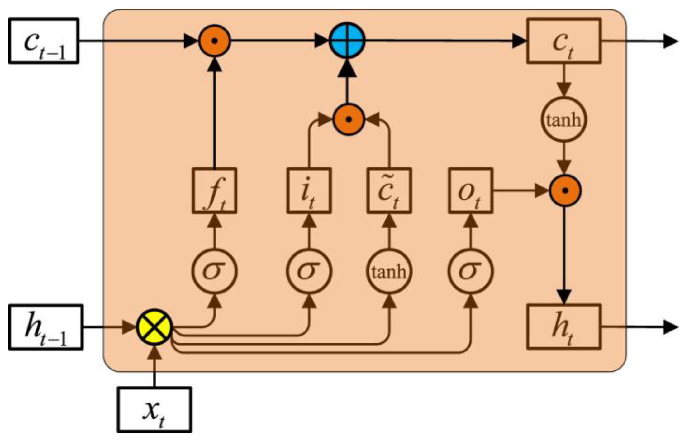
For the RNN model, gradient disappearance and gradient explosion restrict its performance [33]. These two cases are essentially the same, both of which are problems of the continuous multiplication term in extreme cases. Therefore, to alleviate or even eliminate this influence, long short-term memory (LSTM), is one of the variants of RNN. It solved the gradient problems by introducing a gate mechanism to control the flow and loss of features [34]. LSTM is the combination of the RNN structure and the gate structure. It stores information through its unique memory vector, thus eliminating the adverse effects such as gradient explosion existing in RNN. The computation at each time step is depicted by Graves et al. [33] as follows.

$${\mathit{g}}_{\mathit{u}}=\mathsf{\sigma }\left({\mathit{W}}_{\mathit{u}}{\mathit{h}}_{\mathit{t}}{ - 1+\mathit{I}}_{\mathit{u}}{\mathit{x}}_{\mathit{t}}\right)$$

(4)

$${\mathit{g}}_{\mathit{f}}=\mathsf{\sigma }\left({\mathit{W}}_{\mathit{f}}{ \mathit{h}}_{\mathit{t}} {- 1+\mathit{I}}_{\mathit{f}}{\mathit{x}}_{\mathit{t}}\right)$$

(5)

$${\mathit{g}}_{\mathit{o}}=\mathsf{\sigma }\left({\mathit{W}}_{\mathit{o}}{\mathit{h}}_{\mathit{t}} {- 1+\mathit{I}}_{\mathit{o}}{\mathit{x}}_{\mathit{t}}\right)$$

(6)

$${\mathit{g}}_{\mathit{c} }=\tan \mathit{h}\left({\mathit{W}}_{\mathit{c}}{\mathit{h}}_{\mathit{t}} {- 1+\mathit{I}}_{\mathit{c}}{\mathit{x}}_{\mathit{t}}\right)$$

(7)

$${\mathit{m}}_{\mathit{t}}{=\mathit{g}}_{\mathit{f}} \odot { \mathit{m}}_{\mathit{t}}{ - 1+\mathit{g}}_{\mathit{u}} \odot { \mathit{g}}_{\mathit{c}}$$

(8)

$${\mathit{h}}_{\mathit{t}}=\tan \mathit{h}\left({\mathit{g}}_{\mathit{o}} \odot { \mathit{m}}_{\mathit{t}}\right)$$

(9)

where g represents the activation vectors of different gates at different times, h_t is the LSTM units hidden state vector, the logistic sigmoid function is defined by σ, and the element-wise multiplication is represented by ⊙. The recurrent weight matrices are represented by the notation W_u, W_f, W_o, and W_c, whereas the projection matrices are represented by I_u, I_f, I_o, and I_c. The advantages of LSTM are apparent. LSTM has the advantage of excellent sequence modeling ability and solves the problem of RNN gradient through long-term memory function. At the same time, the disadvantage is the lack of parallel processing and time-consuming calculation. Bahdanau et al. [35] proposed an attention mechanism to learn these long-term dependencies. Figure 2 showed how the specific LSTM units are implemented. f_t represents the forgetting gate, i_t is the input gate, and c_t represents the cell status update value.

2.3. Evolutionary Optimization

Particle swarm optimization (PSO), a metaheuristic, stochastic population-based evolutionary optimization algorithm. was chosen for this investigation. Each optimization problem solution is imagined as a bird, called a particle. Each particle in the swarm survives with a velocity and position in solution search space. All particles are searched for the optimal solution in a D-dimensional search space through a swarm by adjusting their speed and direction through the fitness function and sharing their own experience. Formulas of updating movement of an i^th particle in (k + 1)^th iteration are given below [36]:

$${\mathit{v}}_{\mathit{ij}}^{\mathit{k}+1}{=\mathit{v}}_{\mathit{ij}}^{\mathit{k}}{+\mathit{c}}_1\left({\mathit{x}}_{\mathit{ij}}^{\mathit{pb}}{-\mathit{x}}_{\mathit{ij}}^{\mathit{k}}\right){+\mathit{c}}_2\left({\mathit{x}}_{\mathit{ij}}^{\mathit{gb}}{-\mathit{x}}_{\mathit{ij}}^{\mathit{k}}\right)$$

(10)

$${\mathit{x}}_{\mathit{ij}}^{\mathit{k}+1}{=\mathit{x}}_{\mathit{ij}}^{\mathit{k}}{+\mathit{v}}_{\mathit{ij}}^{\mathit{k}+1}$$

(11)

In each iteration, the particle searches for two extremes to update itself. The first extreme value (p_best) is the cognitive behavior determined by the particle’s own best experience traveled so far. The second extreme value (g_best) decides social behavior. g_best is the optimal solution for the whole population. The social coefficient (c₁) and cognitive coefficient (c₂) are parameters to control the behavior of particles and maintain the balance between their exploration and exploitation properties. When they are vector superimposed, the particle’s velocity tends towards global and individual optimizations [37].

2.4. The Proposed Model: LSTM-FCN

This section describes the basic foundation of the hybrid approach, flowchart, algorithms, and detailed architecture of the proposed LSTM-FCN. Figure 3 shows the hybrid model used in this paper, consisting of an FCN block and an LSTM block. The hybrid model is based on the LSTM-FCN network structure proposed by Karim et al. [25].

The fully convolutional block contains three temporal convolutional blocks. These time convolution blocks can extract features from the input data and dig for relationships between the data. It was copied from the original fully convolutional block by Wang et al. [38]. For the whole FCN block, it contains a fully convolutional network, which can adapt to the input of any size. There is also an upsampling deconvolutional layer to reduce the dimensions for further calculation. For the LSTM block, the existence of the gate structure makes its most significant characteristic, memory, perfectly reflected.

Table 1. The Structure of LSTM-FCN Layer.

Layer (Type)	Output Shape	Parameters	Connected to
input_1 (InputLayer)	(None, 1, 5)	0
permute (Permute)	(None, 5, 1)	0	input_1[0][0]
conv1D (Conv1D)	(None, 5, 128)	1152	permute [0][0]
batch_normalization (BatchNor)	(None, 5, 128)	512	conv1D [0][0]
activation (Activation)	(None, 5, 128)	0	batch_normalization [0][0]
conv1D_1 (Conv1D)	(None, 5, 256)	164,096	activation [0][0]
batch_normalization_1 (BatchNor)	(None, 5, 256)	1024	conv1D_1[0][0]
activation_1 (Activation)	(None, 5, 256)	0	batch_normalization_1[0][0]
conv1D_2 (Conv1D)	(None, 5, 128)	98,432	activation_1[0][0]
batch_normalization_2 (BatchNor)	(None, 5, 128)	512	conv1D_2[0][0]
lstm (LSTM)	(None, 8)	448	batch_normalization_2[0][0]
activation_2 (Activation)	(None, 5, 128)	0	input_1[0][0]
dropout (Dropout)	(None, 8)	0	lstm [0][0]
global_average_pooling1d (GlobalPooling)	(None, 128)	0	activation_2[0][0]
concatenate (Concatenate)	(None, 136)	0	dropout [0][0] global_average_pooling1d [0][0]
dense (Dense)	(None, 9)	1233	concatenate [0][0]

illustrates how the proposed model is built and run on the Python platform. For multivariate classification, LSTM-FCN shows outstanding performance in end-to-end processing time series classification [25].

The combination of LSTM and FCN leads to a complicated model, demanding extensive trial and error when setting hyperparameters. So PSO-based LSTM-FCN is used in this investigation.

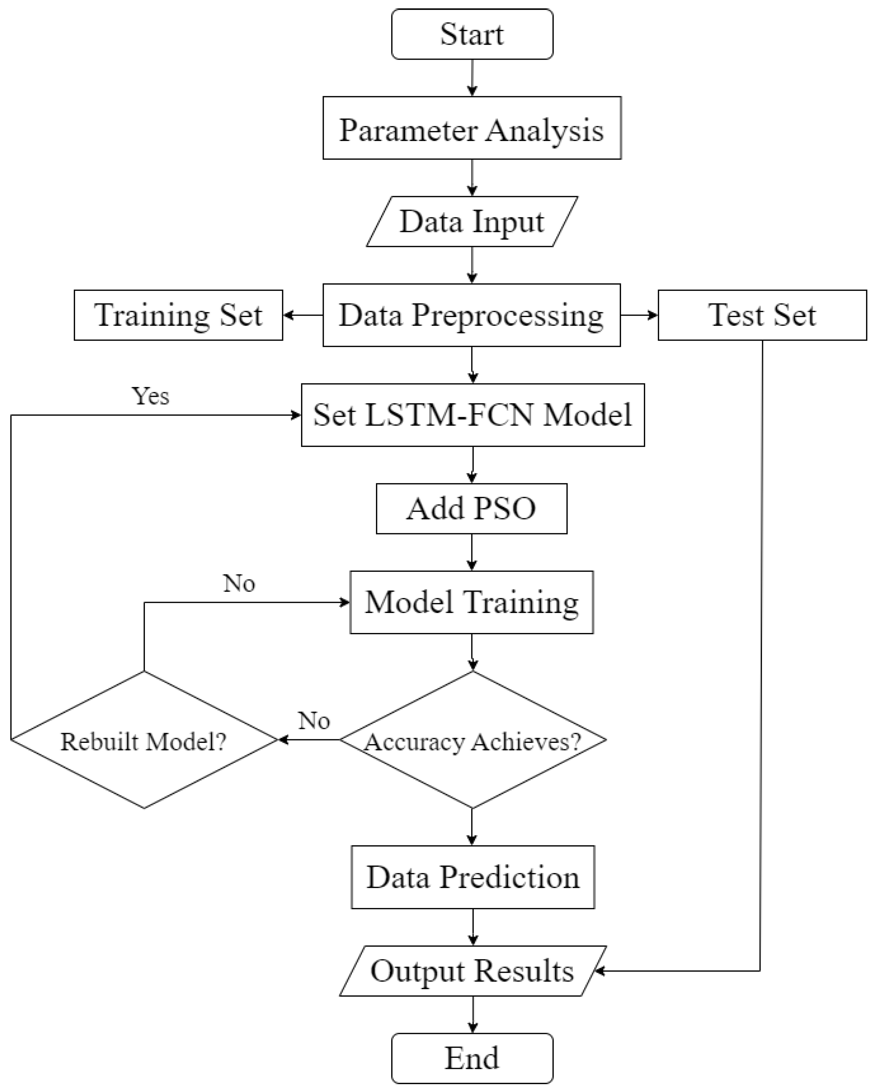
The proposed PSO-based LSTM-FCN method automatically extracts important features of lithology information by connecting LSTM and FCN to minimize the loss of information by modeling sequential information. Figure 4 shows the structure of the proposed PSO-based LSTM-FCN neural network. The proposed method minimizes the loss in parsing so that the pattern information and the order information are not lost. The FCN layer automatically extracts the pattern information. The order of features is learned once again in the LSTM layer. PSO algorithm is adopted to tune the hyperparameters automatically, and the corresponding settings are chosen to encode as particles.

The proposed technique consists of three major components, as presented in Figure 4.

(1)

prepare, analyze, and preprocess the data,

(2)

set the LSTM-FCN model, input the processed parameter data,

(3)

optimize the LSTM-FCN model using the PSO algorithm and output prediction results.

2.5. Model Evaluation Metrics

For the F1-score, precision, Recall, and Jaccard index can be computed efficiently using the confusion matrix. Take a classification problem where the sample has positive, negative, true, and false categories. Four combinations of the predicted results and accurate labels, including true positive (TP), false positive (FP), false negative (FN), and true negative (TN), are chosen to evaluate the model.

Precision is a measure of accuracy, which represents the proportion of positive examples that are true positive examples. It is expressed as,

$$\mathit{Precision}=\mathit{TP}÷\left(\mathit{TP}+\mathit{FP}\right)$$

(12)

Recall represents the proportion of the true positive examples in all examples. It is desirable to have high values for both precision and recall, but often when an algorithm is tuned to increase one, the other decreases:

$$\mathit{Recall}=\mathit{TP}÷\left(\mathit{TP}+\mathit{FN}\right)$$

(13)

F1-score combines the above two metrics and gives the performance index of the classifier [39].

$$\mathit{F}1=\frac{2*\mathit{Precision}*\mathit{Recall}}{\mathit{Precision}+\mathit{Recall}}$$

(14)

Jaccard index, also called Jaccard similarity coefficient, is defined as the size of the intersection of real (y) and predicted values (y_p) divided by the size of the union of those two labels [40].

$$\mathit{Jaccard}=\frac{{\mathit{y}*\mathit{y}}_{\mathit{p}}}{{||\mathit{y}||}^2\times ||{\mathit{y}}_{\mathit{p}}||{}^2}$$

(15)

3. Results

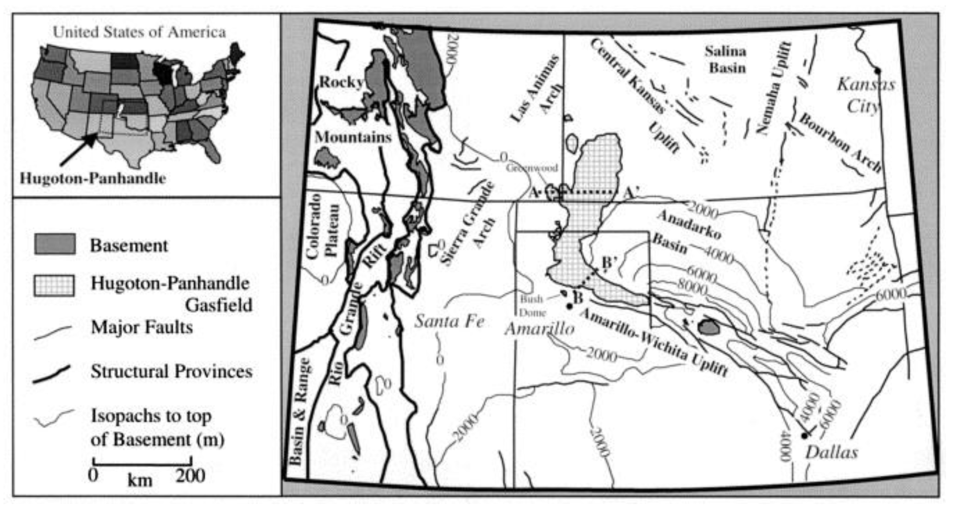
In the study, 3232 data samples from Hugoton Field were used. The Hugoton Field is located in Kansas, Texas, and Oklahoma. The entire field covers about 8500 square miles, it is one of the largest oil and gas fields in the United States. The specific location of the oilfield is shown in the figure below (Figure 5). The main oil pay zones represent thirteen shoaling-upward, fourth-order marine-continental cycles, and have remarkable lateral continuity [41]. The specific log data used is from Shrimplin Well in Hugoton Field and can be downloaded from the field’s official public data.

The Python third-party package TensorFlow was used as the platform to build the lithology classifier. All experiments were conducted on Intel (R) Xeon (R), Silver 4216 CPU @ 2.10 GHz with 10 GB of RAM.

3.1. Data Preparation

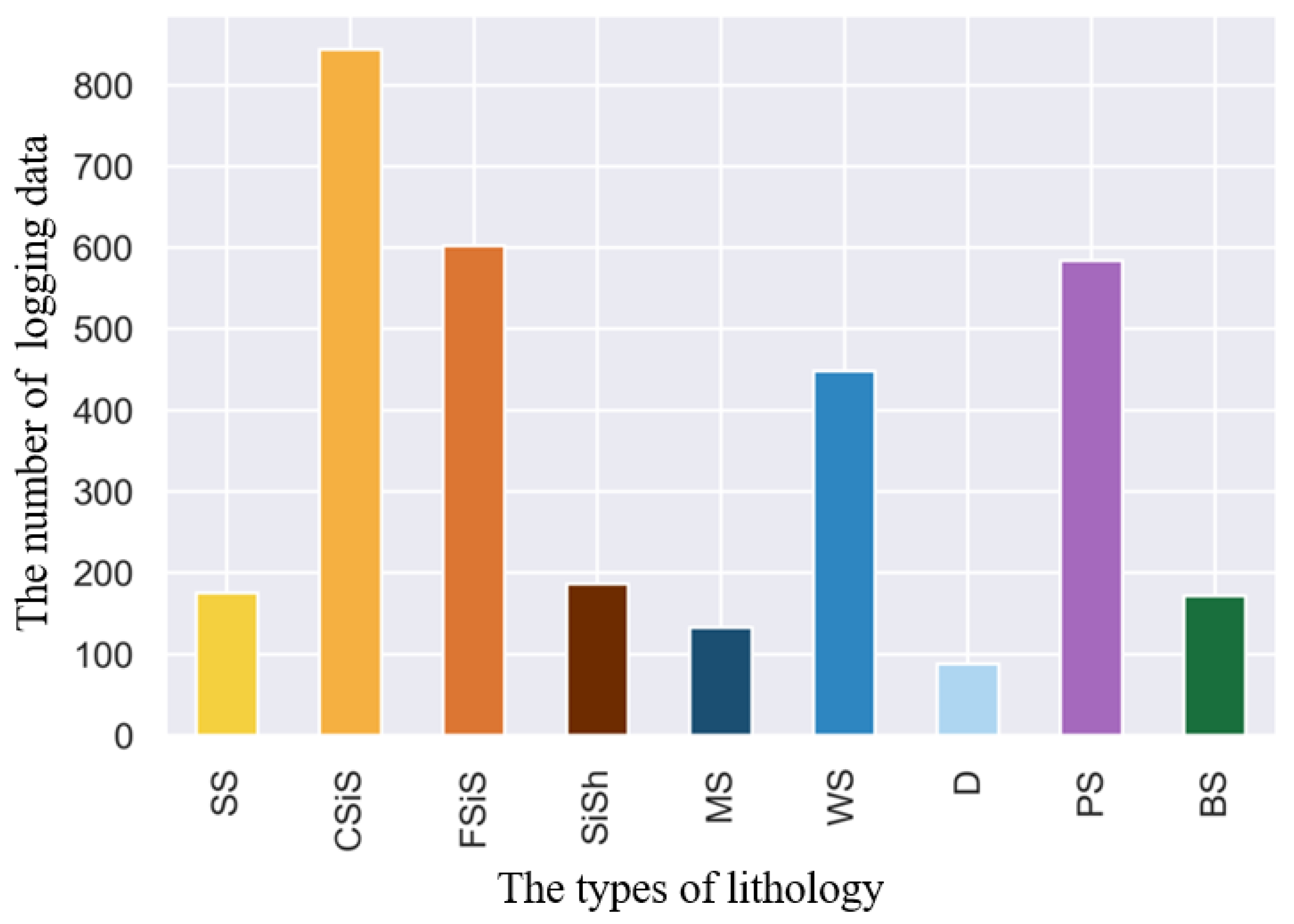
In the dataset, a total of nine lithologies were shown, including sandstone (SS), calcareous siltstone (CSiS), ferruginous siltstone (FSiS), marine_silt_shale (SiSh), mudstone (MS), wackestone (WS), dolomite (D), packstone (PS), bafflestone (BS). More specifically, up to 844 sets of data were distributed in CSiS, 602 sets of data were distributed in FSiS, and the lowest is D, only 88 sets of data are spread (Figure 6).

3.2. Correlation Analysis

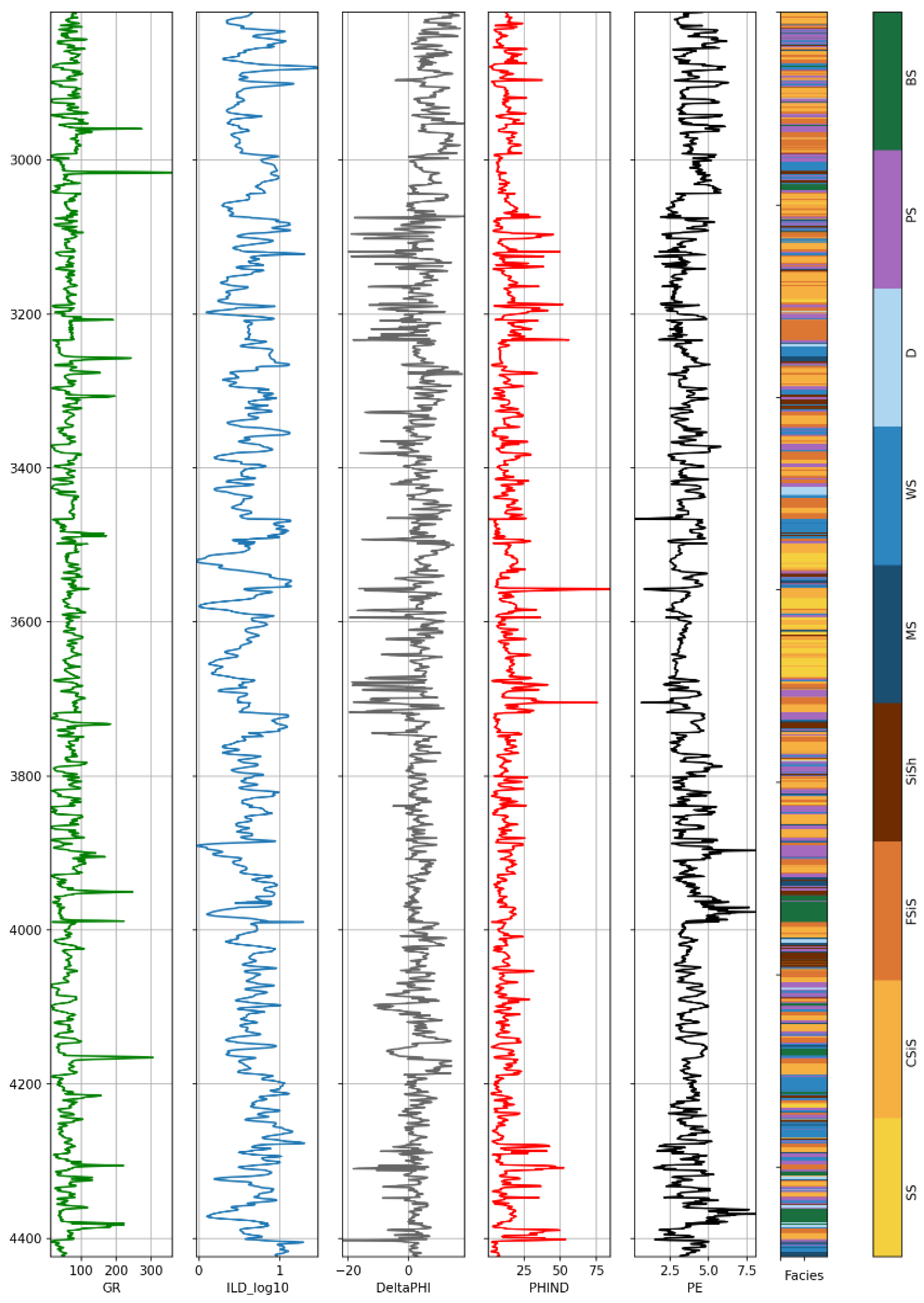
For the study data, phases of each half-foot core sample were studied and matched with well-logging data at the proper location. The characteristic variables included five wireline logging measurements. The five variables are:

GR: determination of natural radioactivity intensity under different lithology.

ILD_log10: the resistivity of rock is measured by electrodes arranged in deep strata.

DeltaPHI: comprehensive logging technology consisting of acoustic transit time logging, neutron logging, and density logging. There are different responses in different lithological formations.

PHIND: using neutron ray to detect the physical properties of rock strata around drilling wells.

PE: the parameter proportional to the electron photoelectric absorption cross section r/Z can better reflect the lithology.

Figure 7 lists the facies, corresponding abbreviated labels, and logging curves of characteristic parameters. Among them, the lithology is arranged in depth order from top to bottom, and different lithology is distinguished by different colors. All logging data can be extracted by classifiers to better classify the lithology. After data preprocessing, such as data normalization and data dimension reduction, the logging data will be input into the classifier for calculation. At the same time, the data will be applied equally to each classifier used in the experiment.

The following figure shows the correlation analysis between the five parameters (Figure 8). The heat map shows the correlation of each two parameters. PHIND and PE have the best negative correlation, with a correlation coefficient of 0.57. They are followed by the pair of ILD_log10 and PE, which has a coefficient of 0.38. Although the correlation does not look very good, the discrete data is more closely related to the actual environment produced in unconventional reservoirs in complex environments.

3.3. Data Normalization

This chapter starts with the data examination (

Table 2. The Data Information.

	Facies	GR	ILD_log10	DeltaPHI	PHIND	PE	Depth
count	3232	3232	3232	3232	3232	3232	3232
mean	4.52	66.14	0.64	3.56	13.48	3.73	3615.75
std	2.55	30.85	0.24	5.23	7.70	0.90	466.57
min	1.00	13.25	−0.03	−21.83	0.55	0.20	2808.00
25%	2.00	46.92	0.49	1.16	8.35	3.10	3211.88
50%	3.00	65.72	0.62	3.50	12.15	3.55	3615.75
75%	7.00	79.63	0.81	6.43	16.45	4.30	4019.63
max	9.00	361.15	1.48	18.60	84.40	8.09	4423.50

). In this part, the basic features of the data set are analyzed and described. This step laid a foundation for the next step of data preprocessing.

Next, the experiment conditioned the data and remove incomplete parts. Then the study scaled data to zero mean and unit variance to make a more efficient model performance. Finally, the experiment divided the processed dataset randomly into training and test data. Through the above steps to data preprocessing, the model can be better fitted and trained.

3.4. Classifiers Comparison

In this part, training 7 machine learning classification models under the same conditions, and compare them with the proposed model to verify the superiority of the model. The study will put these log data into trained, supervised classifiers to predict lithology. All classifier algorithms are implemented based on scikit-learn libraries. The classifiers are:

(1)

Logistic regression (LR)

(2)

Gaussian process classifier (GPC)

(3)

Support vector machines (SVM)

(4)

Multi-layer Perceptron classifier (MLP)

(5)

Convolutional Neural Networks Classifier (CNN)

(6)

Long Short-term Memory (LSTM)

(7)

LSTM-CNN

Two evaluation indexes (F1-score and Jaccard index) were used to provide an essential reference for each model.

The evaluation score shows that the LSTM-FCN model scores better than the rest. It can be seen from the scores of the classifier that the LSTM-FCN model got 0.575 points with the Jaccard index and 0.725 points for the F1-score. Both were the highest scores. The following histogram (Figure 9) is more intuitive to show that for the predictive ability, the LSTM-FCN model is the best classifier in the study.

3.5. The PSO-LSTM-FCN Model

In the experiment, due to the lack of correlation between the original well log data, only using the LSTM-FCN model is not satisfactory. The experiment solved this problem by using the PSO algorithm in the model.

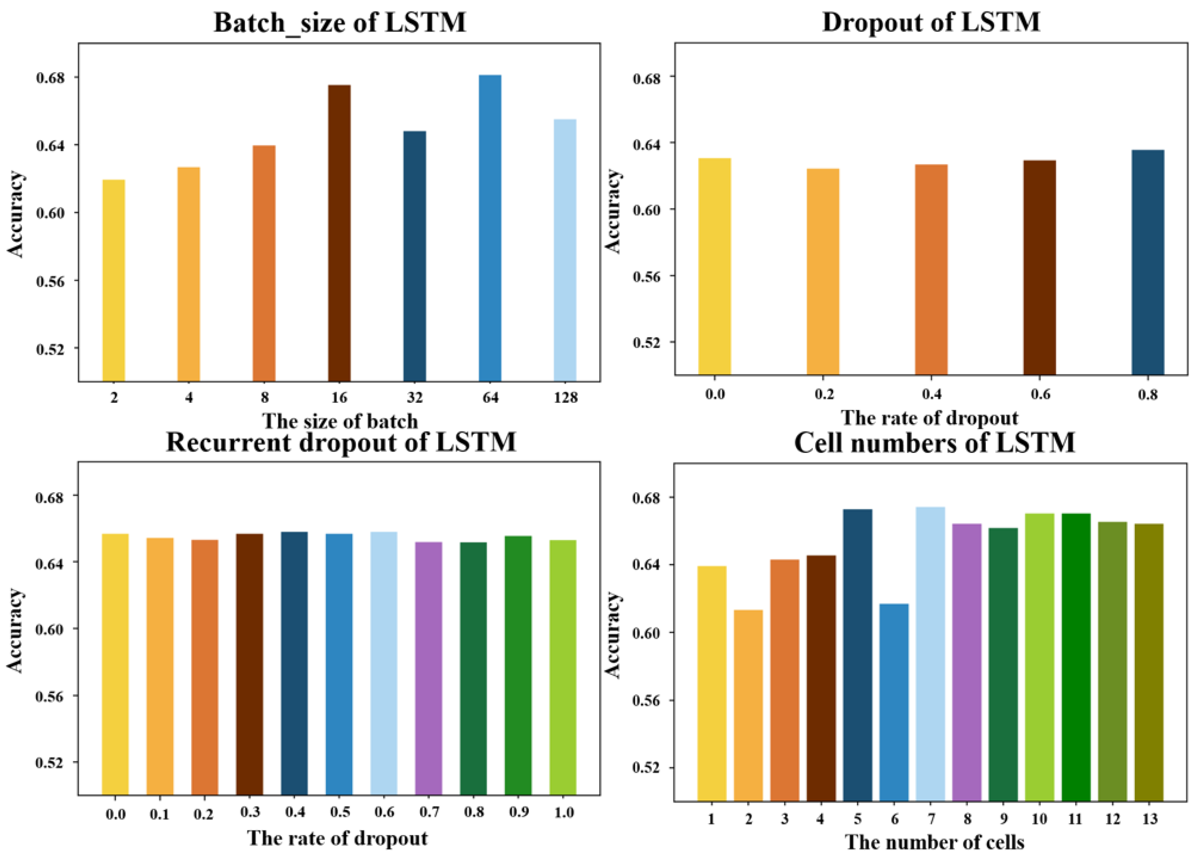
Before the optimizer is run, the parameters to be optimized are first screened. Based on the parameter’s physical meaning and the model’s requirements, the experiment selected four main parameters from 24 parameters for sensitivity analysis, including recurrent_dropout, num_cells, batch_size, and dropout.

The results of sensitivity analysis for selected parameters are shown in the following figure (Figure 10). From the histogram, the change of recurrent_dropout and drop out has almost no effect on the accuracy of the model. Similarly, when num_cells is greater than 8, its influence on accuracy is negligible. Therefore, in the subsequent PSO optimization, batch_size in the LSTM parameters is first selected for optimization.

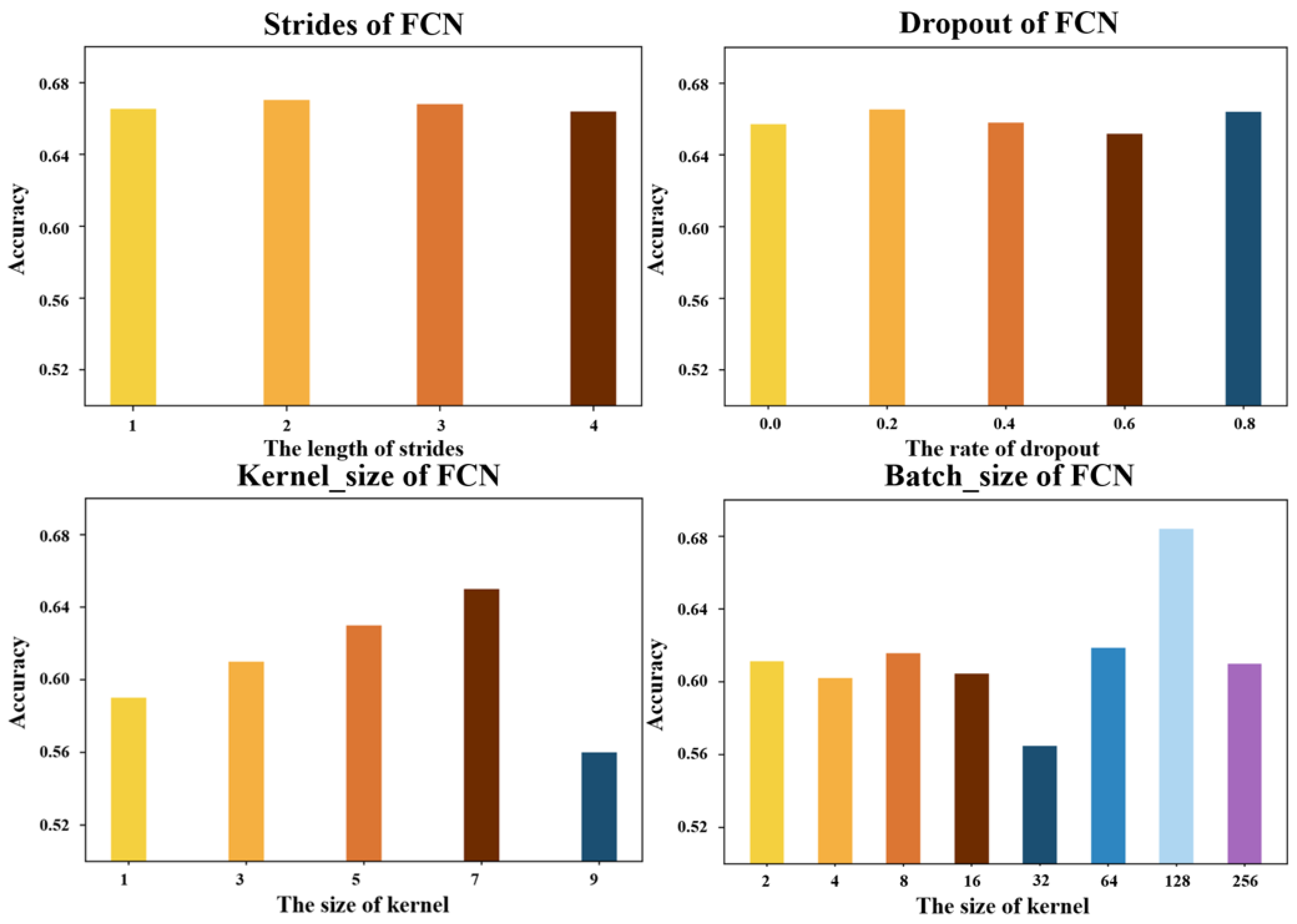
Similarly, for the fully convolutional layer, of all the parameters, kernel_size, batch_size, drop out, and strides are selected. Sensitivity analysis for these parameters is shown in the figure (Figure 11). The change of strides and dropout almost does not affect the evolution of accuracy. The remaining two parameters change the accuracy to some extent. Therefore, for the fully convolutional layer, kernel_size and batch_size were initially selected for PSO optimization.

Then the different combinations are input into the model with varying numbers of layers (1, 2, 3, 4, 5) to calculate the accuracy, and the accuracy of the same layers is averaged. The result shows that the average accuracy of the three-layer FCN has the best performance (Figure 12).

According to the results of sensitivity analysis and LSTM-FCN layer optimization investigation [27], the layer number of the model and the selection range of the feature parameters are determined. Based on this, the experiment mixed the three-layer FCN model with the LSTM model and conducted PSO optimization on the following seven parameters. The following table (

Table 3. Parameters Used in PSO Optimization.

Parameter	Physical Significance	Range
The batch size of the first layer of FCN	The number of samples taken for one training in the first convolutional layer of FCN	64–256
The batch size of the second layer of FCN	The number of samples taken for one training in the second convolutional layer of FCN	64–256
The batch size of the third layer of FCN	The number of samples taken for one training in the third convolutional layer of FCN	64–256
The kernel size of the first layer of FCN	The number of steps in the first convolutional layer of FCN	1–10
The kernel size of the second layer of FCN	The number of steps in the second convolutional layer of FCN	1–10
The kernel size of the third layer of FCN	The number of steps in the third convolutional layer of FCN	1–10
The batch size of LSTM	The number of samples taken for one training of LSTM	32–128

) shows each parameter’s physical meanings and recommended ranges. In particular, although PSO is looking for the optimal solution randomly, it cannot select the parameter range randomly. Otherwise, the accuracy will fall into the dilemma of local optimization and getting the desired result. In the actual study process, it is found that the optimization range of the selected parameters is shown in the table below, which is set to avoid the significant decrease in accuracy caused by overfitting.

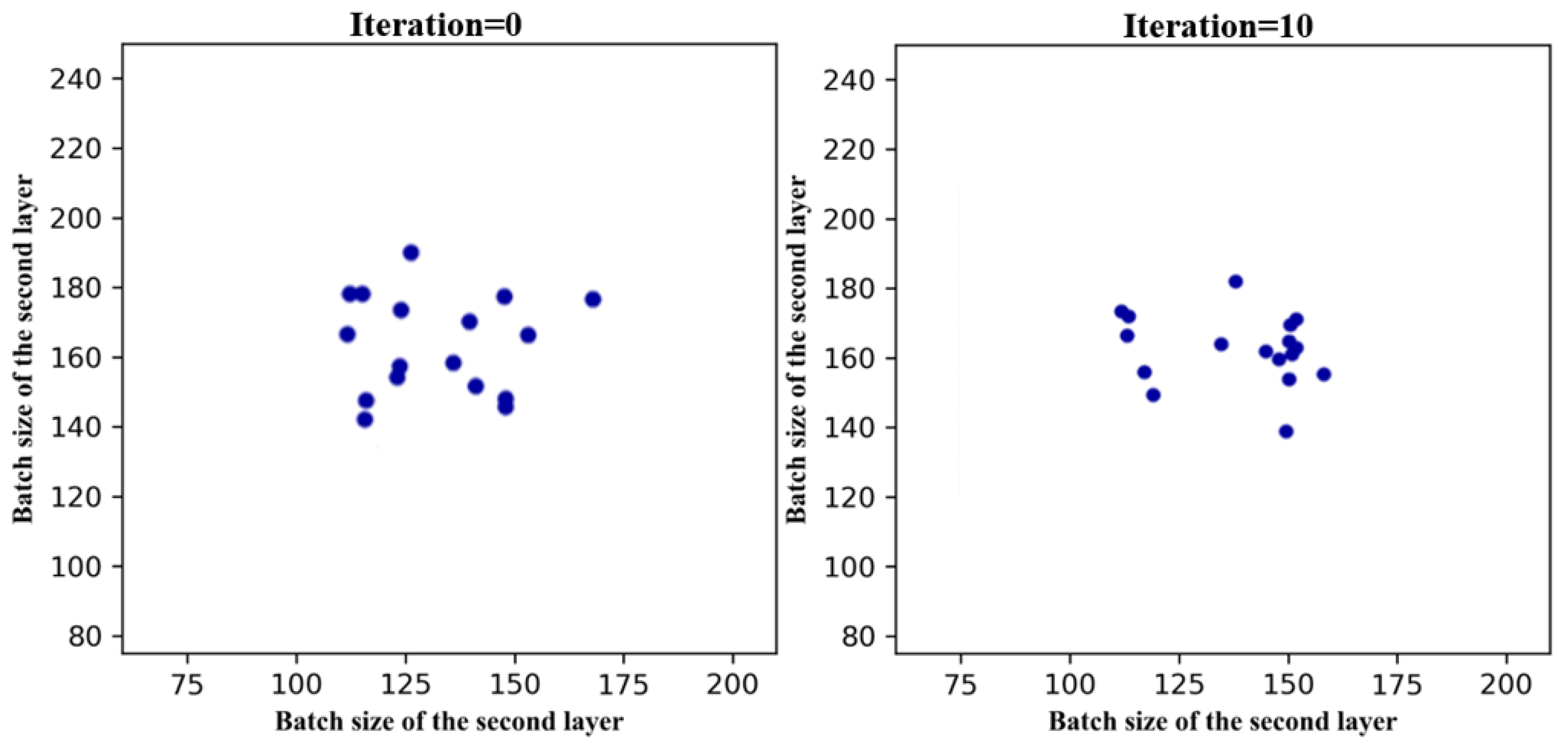
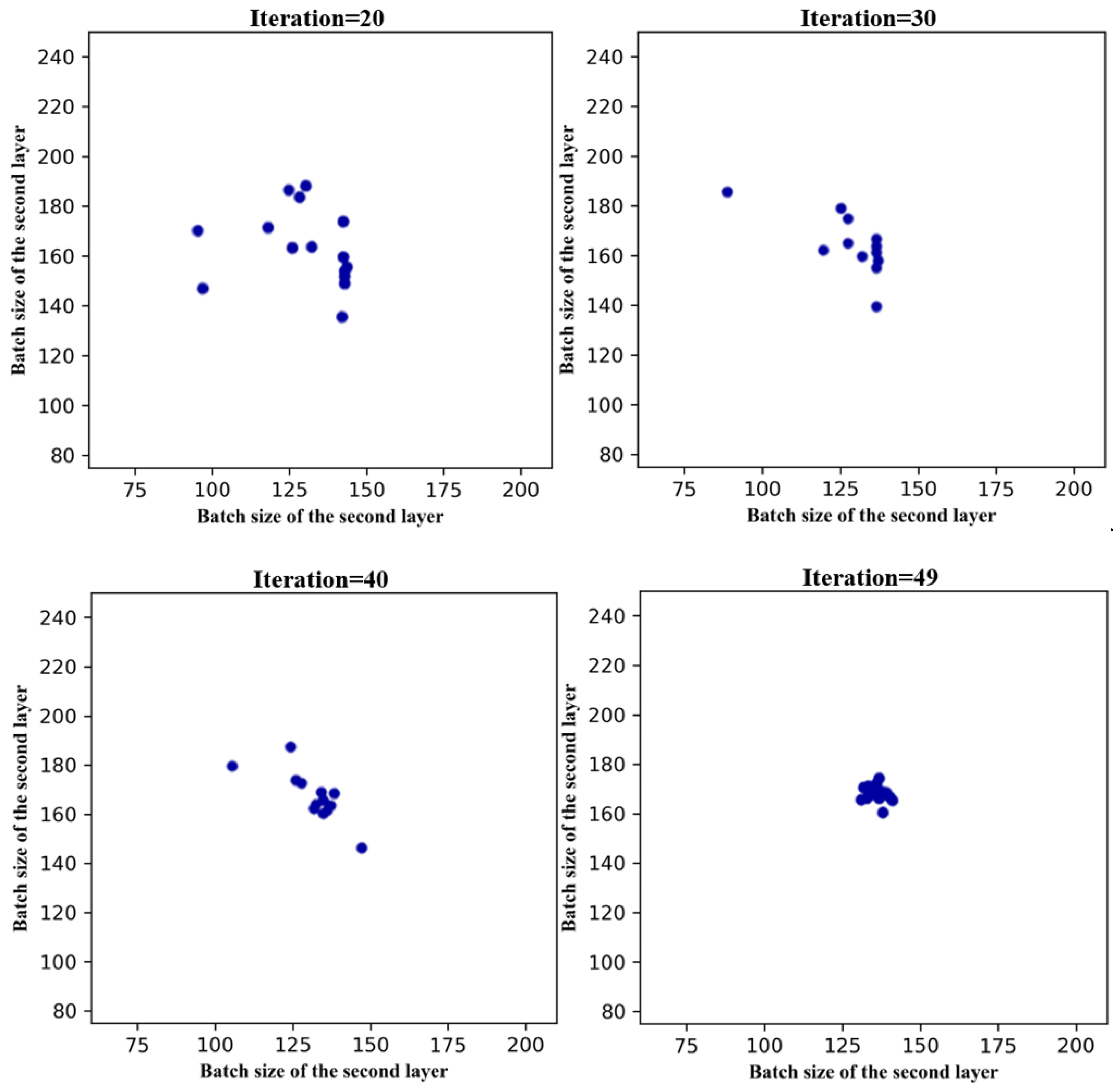
Optimizing the parameters in the PSO process is shown in Figure 13. By selecting the first two layers of the FCN for demonstration, the abscissa and ordinate are the values of the two layers of the FCN, respectively. In a total of 50 iterations, Figure 13 records the position of the parameters after every ten iterations. It shows how the parameters are optimized to the best position.

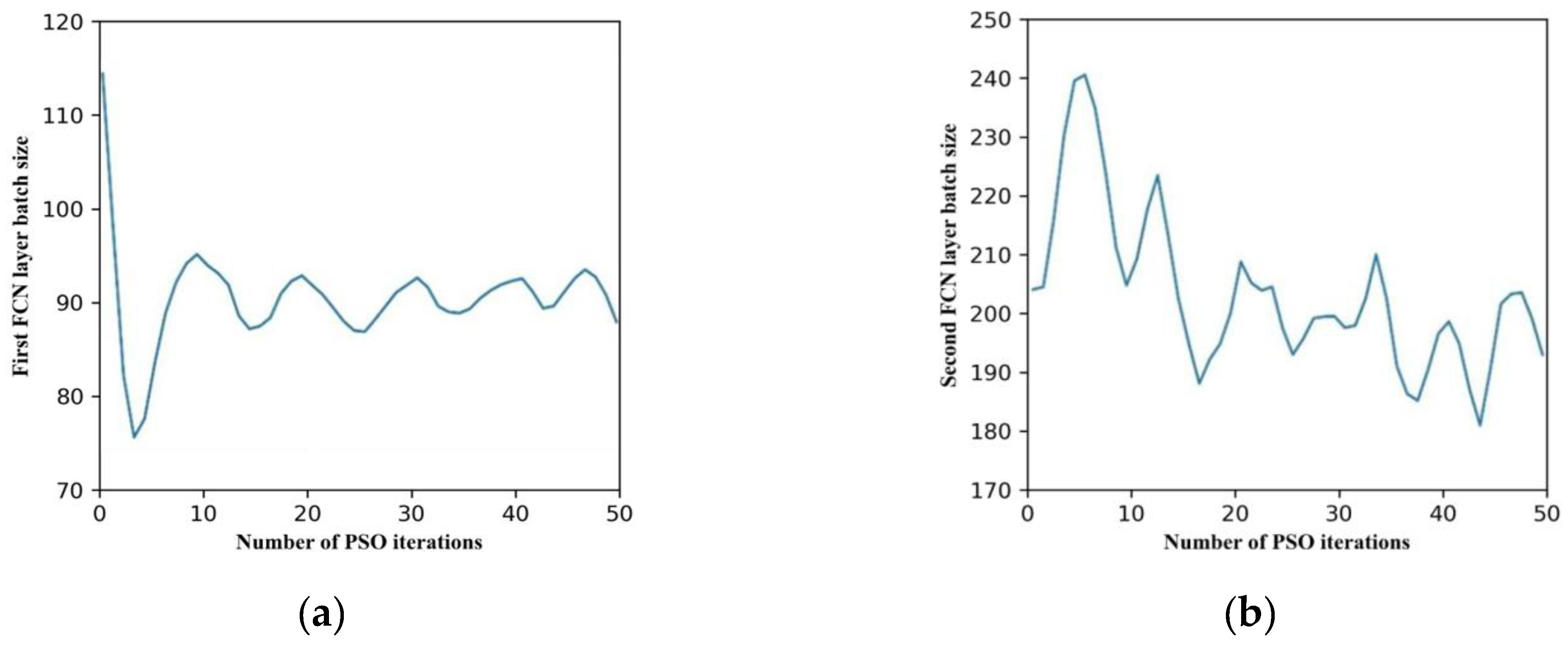
Then, the optimization process of each parameter with iteration is shown in Figure 14.

Table 4. The Confusion Matrix of the PSO-LSTM-FCN Model.

Pred True	SS	CSiS	FSiS	SiSh	MS	WS	D	PS	BS	Total
SS	22	3			1					26
CSiS	8	107	48		1	1		2		167
FSiS		8	109	1		3	1			122
SiSh		4	3	20		7		1		35
MS		1	3	1	5	11		3		24
WS		1		3		67	1	16	1	89
D		1					14	2		17
PS	1	3	3	1	1	9	3	111	7	139
BS						2	1	2	23	28
Precision	0.81	0.94	0.76	0.87	0.72	0.77	0.80	0.91	0.84	0.85
Recall	0.95	0.74	0.99	0.67	0.61	0.85	0.82	0.90	0.92	0.84
F1-score	0.87	0.83	0.86	0.76	0.71	0.86	0.80	0.90	0.88	0.83

shows the confusion matrix, which is a standard format for precision evaluation, of the PSO-LSTM-FCN network model for the classification results of test sets. In the matrix, the columns represent the predicted categories, the rows represent the true attribution categories of the data, and the specific numbers in the table represent the rate of real data accurately predicted to be of these categories. As can be seen from the Table 4, lithologic CSiS, SiSh, PS, and BS achieved good identification effects. The F1-score values and the recall values of lithologic SiSh, D, and MS are lower than those of other lithologies. The reason for this phenomenon may be due to the small number of training samples affecting the accuracy of the model training.

In this part, after the PSO optimization process, the model precision accuracy rate reached 0.85. It has increased by 12.5% compared with that before PSO optimization.

4. Discussion

In terms of processing discrete data, the PSO-LSTM-FCN model proposed in this paper achieves a better effect than previous classifiers. However, the proposed model also has limitations. On the one hand, the lack of interpretability of the model has an impact on the detection of model bias and model reliability; On the other hand, compared with existing mature applications, the accuracy of the model needs to be improved.

The interpretability of the model can be explained by fitting the model to an interpretable algorithm. This method can fully explain the operation of the model from the whole or the part. Using this method can not only improve the reliability of the model, but also make the model more friendly to non-specialists [42].

For accuracy improvement, there is one way to solve this from an optimization perspective. By combing the design process, it is found that the selection of FCN layers in the process of PSO optimization is not particularly rigorous. Just by adding a control variable to the method of this experiment data, it is too simple to determine the number of layers, and it is not universal. So after investigating the optimization techniques, the model’s accuracy will be more accurate by optimizing the number of layers through multi-layer PSO [43]. Multi-layer PSO is a new PSO technology. Through the superposition of two layers of PSO, one layer optimizes the classifier’s parameters, and the other layer optimizes the number of layers of the classifier, to dynamically select the optimal number of layers. In this way, the proposed model can achieve higher accuracy.

5. Conclusions

In this paper, a new method of lithology prediction based on the PSO-LSTM-FCN model is innovatively proposed.

• The paper investigated the application status of lithology identification and discovered the shortcoming of existing technology. On this basis, the paper proposed the PSO-LSTM-FCN model for lithology identification which is suitable for nonlinear discrete data.
• The experiment compared the LSTM-FCN model with seven classifiers. The F1-score and the Jaccard index showed that the proposed new model achieves 0.575 and 0.725 scores, surpassing all previous classifiers. Therefore, the LSTM-FCN model is selected for optimization and used to identify lithology.
• The experiment selected the parameters to be optimized through sensitivity analysis. In the LSTM layer, the analysis showed that batch_size had a greater influence on the accuracy. And in the FCN layer, the kernel_size and batch_size are to be selected. Then, through the PSO optimization, the accuracy of the model reaches 85%, greatly improving the accuracy of the machine learning model in lithology identification.

References

1. Valentín, M.B.; Bom, C.R.; Coelho, J.M.; Correia, M.D.; de Albuquerque, M.P.; de Albuquerque, M.P.; Faria, E.L. A deep residual convolutional neural network for automatic lithological facies identification in Brazilian pre-salt oilfield wellbore image logs. J. Pet. Sci. Eng. 2019, 179, 474–503. [Google Scholar] [CrossRef]
2. Chaki, S.; Routray, A.; Mohanty, W.K. A probabilistic neural network (PNN) based framework for lithology classification using seismic attributes. J. Appl. Geophys. 2022, 199, 104578. [Google Scholar] [CrossRef]
3. McPhee, C.; Reed, J.; Zubizarreta, I. Core Analysis: A Best Practice Guide; Elsevier: Amsterdam, The Netherlands, 2015. [Google Scholar]
4. Młynarczuk, M.; Górszczyk, A.; Ślipek, B. The application of pattern recognition in the automatic classification of microscopic rock images. Comput. Geosci. 2013, 60, 126–133. [Google Scholar] [CrossRef]
5. Migeon, S.; Weber, O.; Faugeres, J.C.; Saint-Paul, J. SCOPIX: A new X-ray imaging system for core analysis. Geo-Mar. Lett. 1998, 18, 251–255. [Google Scholar] [CrossRef]
6. Mitchell, J.; Chandrasekera, T.; Holland, D.; Gladden, L.; Fordham, E. Magnetic resonance imaging in laboratory petrophysical core analysis. Phys. Rep. 2013, 526, 165–225. [Google Scholar] [CrossRef]
7. Martin, K.G.; Carr, T.R. Developing a quantitative mudrock calibration for a handheld energy dispersive X-ray fluorescence spectrometer. Sediment. Geol. 2020, 398, 105584. [Google Scholar] [CrossRef]
8. Thomas, A.; Rider, M.; Curtis, A.; MacArthur, A. Automated lithology extraction from core photographs. First Break 2011, 29, 103–109. [Google Scholar] [CrossRef]
9. Yang, J.; Wang, M.; Li, M.; Yan, Y.; Wang, X.; Shao, H.; Yu, C.; Wu, Y.; Xiao, D. Shale lithology identification using stacking model combined with SMOTE from well logs. Unconv. Resour. 2022, 2, 108–115. [Google Scholar] [CrossRef]
10. Gifford, C.M.; Agah, A. Collaborative multi-agent rock facies classification from wireline well log data. Eng. Appl. Artif. Intell. 2010, 23, 1158–1172. [Google Scholar] [CrossRef]
11. Kuhn, S.; Cracknell, M.J.; Reading, A.M. Lithological mapping in the Central African Copper Belt using Random Forests and clustering: Strategies for optimised results. Ore Geol. Rev. 2019, 112, 103015. [Google Scholar] [CrossRef]
12. Liu, Z.; Cao, J.; You, J.; Chen, S.; Lu, Y.; Zhou, P. A lithological sequence classification method with well log via SVM-assisted bi-directional GRU-CRF neural network. J. Pet. Sci. Eng. 2021, 205, 108913. [Google Scholar] [CrossRef]
13. Zhang, H.; Yu’nan, L. Research on identification model of element logging shale formation based on IPSO-SVM. Petroleum 2022, 8, 185–191. [Google Scholar] [CrossRef]
14. Raeesi, M.; Moradzadeh, A.; Ardejani, F.D.; Rahimi, M. Classification and identification of hydrocarbon reservoir lithofacies and their heterogeneity using seismic attributes, logs data and artificial neural networks. J. Pet. Sci. Eng. 2012, 82–83, 151–165. [Google Scholar] [CrossRef]
15. Zhang, P.Y.; Sun, J.M.; Jiang, Y.J.; Gao, J.S. Deep Learning Method for Lithology Identification from Borehole Images. In Proceedings of the 79th EAGE Conference and Exhibition 2017, Paris, France, 12–15 June 2017; European Association of Geoscientists & Engineers: Utrecht, The Netherlands, 2017; Volume 2017, pp. 1–5. [Google Scholar]
16. Antle, R. Automated core fracture characterization by computer vision and image analytics of CT images. In Proceedings of the SPE Oklahoma City Oil and Gas Symposium, Oklahoma City, OK, USA, 9–10 April 2019. SPE-195181-MS. [Google Scholar] [CrossRef]
17. Xu, Z.; Shi, H.; Lin, P.; Liu, T. Integrated lithology identification based on images and elemental data from rocks. J. Pet. Sci. Eng. 2021, 205, 108853. [Google Scholar] [CrossRef]
18. Xu, Z.; Ma, W.; Lin, P.; Shi, H.; Pan, D.; Liu, T. Deep learning of rock images for intelligent lithology identification. Comput. Geosci. 2021, 154, 104799. [Google Scholar] [CrossRef]
19. Lin, J.; Li, H.; Liu, N.; Gao, J.; Li, Z. Automatic lithology identification by applying LSTM to logging data A case study in X tight rock reservoirs. IEEE Geosci. Remote Sens. Lett. 2020, 18, 1361–1365. [Google Scholar] [CrossRef]
20. Li, K.; Xi, Y.; Su, Z.; Zhu, J.; Wang, B. Research on reservoir lithology prediction method based on convolutional recurrent neural network. Comput. Electr. Eng. 2021, 95, 107404. [Google Scholar] [CrossRef]
21. Liu, Z.; Li, L.; Fang, X.; Qi, W.; Shen, J.; Zhou, H.; Zhang, Y. Hard-rock tunnel lithology prediction with TBM construction big data using a global-attention-mechanism-based LSTM network. Autom. Constr. 2021, 125, 103647. [Google Scholar] [CrossRef]
22. Shi, M.; Yang, B.; Chen, R.; Ye, D. Logging curve prediction method based on CNN-LSTM-attention. Earth Sci. Inform. 2022, 15, 2119–2131. [Google Scholar] [CrossRef]
23. Zhang, F.; Deng, S.; Wang, S.; Sun, H. Convolutional neural network long short-term memory deep learning model for sonic well log generation for brittleness evaluation. Interpretation 2022, 10, T367–T378. [Google Scholar] [CrossRef]
24. Liu, J.; Liu, J. Integrating deep learning and logging data analytics for lithofacies classification and 3D modeling of tight sandstone reservoirs. Geosci. Front. 2022, 13, 101311. [Google Scholar] [CrossRef]
25. Karim, F.; Majumdar, S.; Darabi, H.; Chen, S. Lstm fully convolutional networks for time series classification. IEEE Access 2017, 6, 1662–1669. [Google Scholar] [CrossRef]
26. Budak, Ü.; Cömert, Z.; Rashid, Z.N.; Şengür, A.; Çıbuk, M. Computer-aided diagnosis system combining FCN and Bi-LSTM model for efficient breast cancer detection from histopathological images. Appl. Soft Comput. 2019, 85, 105765. [Google Scholar] [CrossRef]
27. Ortego, P.; Diez-Olivan, A.; Del Ser, J.; Veiga, F.; Penalva, M.; Sierra, B. Evolutionary LSTM-FCN networks for pattern classification in industrial processes. Swarm Evol. Comput. 2020, 54, 100650. [Google Scholar] [CrossRef]
28. Soltani, Z.; Imamalipour, A. An improved classification of mineralized zones using particle swarm optimization: A case study from Dagh-Dali ZnPb (±Au) prospect, Northwest Iran. Geochemistry 2022, 82, 125850. [Google Scholar] [CrossRef]
29. Min, X.; Pengbo, Q.; Fengwei, Z. Research and application of logging lithology identification for igneous reservoirs based on deep learning. J. Appl. Geophys. 2020, 173, 103929. [Google Scholar] [CrossRef]
30. Liang, H.; Chen, H.; Guo, J.; Bai, J.; Jiang, Y. Research on lithology identification method based on mechanical specific energy principle and machine learning theory. Expert Syst. Appl. 2022, 189, 116142. [Google Scholar] [CrossRef]
31. Ren, Q.; Zhang, H.; Zhang, D.; Zhao, X.; Yan, L.; Rui, J.; Zeng, F.; Zhu, X. A framework of active learning and semi-supervised learning for lithology identification based on improved naive Bayes. Expert Syst. Appl. 2022, 202, 117278. [Google Scholar] [CrossRef]
32. Pascanu, R.; Gulcehre, C.; Cho, K.; Bengio, Y. How to construct deep recurrent neural networks. arXiv 2013, arXiv:1312.6026. [Google Scholar] [CrossRef]
33. Kawakami, K. Supervised Sequence Labelling with Recurrent Neural Networks; Technical University of Munich: Singapore, 2012; Volume 385, ISBN 978-3-642-24797-2. [Google Scholar]
34. Hochreiter, S.; Schmidhuber, J. Long short-term memory. Neural Comput. 1997, 9, 1735–1780. [Google Scholar] [CrossRef]
35. Bahdanau, D.; Cho, K.; Bengio, Y. Neural machine translation by jointly learning to align and translate. arXiv 2014, arXiv:1409.0473. [Google Scholar]
36. Buyukada, M. Co-combustion of peanut hull and coal blends: Artificial neural networks modeling, particle swarm optimization and Monte Carlo simulation. Bioresour. Technol. 2016, 216, 280–286. [Google Scholar] [CrossRef]
37. Liu, Y.; Dai, J.; Zhao, S.; Zhang, J.; Shang, W.; Li, T.; Zheng, Y.; Lan, T.; Wang, Z. Optimization of five-parameter BRDF model based on hybrid GA-PSO algorithm. Optik 2020, 219, 164978. [Google Scholar] [CrossRef]
38. Wang, Z.; Yan, W.; Oates, T. Time Series Classification from Scratch with Deep Neural Networks: A Strong Baseline. In Proceedings of the 2017 International Joint Conference on Neural Networks (IJCNN), Anchorage, AK, USA, 14–19 May 2017; pp. 1578–1585. [Google Scholar] [CrossRef] [Green Version]
39. Saputelli, L.; Celma, R.; Boyd, D.; Shebl, H.; Gomes, J.; Bahrini, F.; Escorcia, A.; Pandey, Y. Deriving Permeability and Reservoir Rock Typing Supported with Self-Organized Maps SOM and Artificial Neural Networks ANN—Optimal Workflow for Enabling Core-Log Integration. In Proceedings of the SPE Reservoir Characterisation and Simulation Conference and Exhibition, Abu Dhabi, United Arab Emirates, 17–19 September 2019. SPE-196704-MS. [Google Scholar] [CrossRef]
40. Krebs, C.J. Ecological Methodology; No. 574.5072 K7; Addison-Wesley Educational Publishers, Inc.: Menlo Park, CA, USA, 1999. [Google Scholar]
41. Dubois, M.K.; Byrnes, A.P.; Bohling, G.C.; Doveton, J.H. Multiscale geologic and petrophysical modeling of the giant Hugoton gas field (Permian), Kansas and Oklahoma. In Giant Hydrocarbon Reservoirs of the World: From Rocks to Reservoir Characterization and Modeling; AAPG Memoir 88/SEPM Special Publication: London, UK, 2006; pp. 307–353. [Google Scholar] [CrossRef]
42. Kim, J.; Lee, G.; Lee, S.; Lee, C. Towards expert–machine collaborations for technology valuation: An interpretable machine learning approach. Technol. Forecast. Soc. Chang. 2022, 183, 121940. [Google Scholar] [CrossRef]
43. Singh, P.; Chaudhury, S.; Panigrahi, B.K. Hybrid MPSO-CNN: Multi-level Particle Swarm optimized hyperparameters of Convolutional Neural Network. Swarm Evol. Comput. 2021, 63, 100863. [Google Scholar] [CrossRef]
Figure 1. The structure of the RNN Model.
Energies 16 02135 g001
Figure 2. The Structure of the LSTM Model.
Energies 16 02135 g002
Figure 3. The LSTM-FCN Framework.
Energies 16 02135 g003
Figure 4. Flow Chart of Experiment.
Energies 16 02135 g004
Figure 5. The Location of The Hugoton Field.
Energies 16 02135 g005
Figure 6. Distribution of Training Data by Facies.
Energies 16 02135 g006
Figure 7. Well Log for Each Characteristic Parameter.
Energies 16 02135 g007
Figure 8. Pearson Correlation Diagram (heatmap).
Energies 16 02135 g008
Figure 9. Evaluation Criteria for Different Classifiers.
Energies 16 02135 g009
Figure 10. Sensitivity Analysis of LSTM Parameters.
Energies 16 02135 g010
Figure 11. Sensitivity Analysis of FCN layer Parameters.
Energies 16 02135 g011
Figure 12. The Average Value of the Accuracy Rate.
Energies 16 02135 g012
Figure 13. PSO Optimization Process.
Energies 16 02135 g013aEnergies 16 02135 g013b
Figure 14. The Optimization Process of Each Parameter. (a) The first layer batch size of FCN. (b) The second layer batch size of FCN. (c) The third layer batch size of FCN. (d) The first layer kernel size of FCN. (e) The second layer kernel size of FCN. (f) The third layer kernel size of FCN. (g) The batch size of LSTM.
Energies 16 02135 g014aEnergies 16 02135 g014b