Article

Mathematical Modeling Study of Pressure Loss in the Flow Channels of Additive Manufacturing Aviation Hydraulic Valves

College of Mechanical and Electrical Engineering, Nanjing University of Aeronautics and Astronautics, Nanjing 210016, China
*
Authors to whom correspondence should be addressed.
Energies 2023, 16(4), 1788; https://doi.org/10.3390/en16041788
Submission received: 1 January 2023 / Revised: 19 January 2023 / Accepted: 20 January 2023 / Published: 10 February 2023

Abstract

:
The application of additive manufacturing in the field of aviation hydraulics greatly improves the design freedom of hydraulic valve internal flow channels. Pressure loss in hydraulic valve internal flow channels is a primary factor that designers need to consider, and the rapid prediction of pressure loss is very helpful for flow channel design. At present, most studies only focus on how much the pressure loss in an additive manufacturing (AM) hydraulic channel is reduced compared with an original hydraulic channel, and a mathematical model of pressure loss in an AM curved channel is still lacking. In this paper, the pressure loss in a curved flow channel was firstly studied, and the main parameters affecting the pressure loss were determined using the dimensionless analysis method. Using computational fluid dynamics simulation, the relationships between the flow channel diameter, the flow channel length, the flow channel curvature radius, the fluid velocity and pressure loss were studied. According to the multiple regression analysis method, the mathematical model of pressure loss in aviation hydraulic channels was developed, and the model was solved based on the orthogonal experimental results. The pressure loss in the flow channel samples fabricated using selective laser melting was tested, and the results showed that the average error between the test results and the mathematical model calculation results was 7.72%. This model can be used to quickly predict the pressure loss in curved flow channels in the aviation hydraulic field.

1. Introduction

A hydraulic valve is a kind of hydraulic component operated by pressure oil. It is controlled by pressure oil and is usually used for reversing and switching oil in a hydraulic system. Drilling and milling methods have been used to process traditional hydraulic valves’ internal flow channels [1,2], which cause many right-angle turns in flow channels. In essence, right-angle turns are the main cause of pressure loss in a flow channel. The appearance of additive manufacturing (AM) has changed the traditional layout of flow channels. AM technology can produce complex valve blocks with unique design attributes [3,4,5,6], for example, reductions in the mass of hydraulic valve blocks, reductions in the volume of hydraulic valve blocks, improvements in the design freedom of the flow channels and increases in the compactness of the flow channels [7,8,9].
AM is a technology that uses the layer-upon-layer stacking of materials to fabricate the structure of parts [10]. At present, AM technology has been used to replace traditional manufacturing for many products in aerospace [11,12], national defense [13], robotics [14] and medical industries [15]. AM is widely used in parts with functional fluid flow channels, such as hydraulic valves, nozzles, valves, actuators, molds with conformal cooling channels and heat exchangers [16,17].
Selective laser melting (SLM) is one of the main technical approaches in the AM of metal materials. This technology selects a laser as the energy source and scans the metal powder bed layer by layer according to the path planned in the 3D CAD slice model. The scanned metal powder can achieve the effect of metallurgical combination through melting and solidification, and it can finally obtain the metal parts designed by the model. There have been several efforts to improve hydraulic valve blocks by redesigning them for SLM in recent years. Schmelzle et al. redesigned a main landing gear test hydraulic valve block in the Bell-Boeing V-22 Osprey aircraft [18]. Compared with the original plan, the mass of the redesigned hydraulic valve block was reduced by 60%. Diegel et al. redesigned a conventionally manufactured hydraulic valve block, and the mass of the hydraulic valve block was reduced by 91% [19].
In addition to mass reductions in hydraulic valve blocks, the optimized design of flow channels has also drawn interest. Chekurov and Lantela redesigned a digital hydraulic valve based on AM, and the pressure loss in the redesigned hydraulic valve was reduced by 49% [20]. Aiman et al. used computational fluid dynamics (CFD) and fluid structure interaction simulation to optimize the design of the flow channel of a hydraulic manifold, and the pressure loss in the redesigned flow channel was reduced by 25% [21]. Cooper et al. redesigned traditional hydraulic valve internal flow channels for Red Bull Technology Formula 1 racing using direct metal laser sintering (DMLS) to manufacture a hydraulic valve which, compared with the traditional hydraulic valve, had a flow rate which was increased by 250% [22]. Although the redesigned flow channels have a more compact layout, how to ensure the minimum pressure loss while using these compact layouts is a big challenge.
At present, some scholars have carried out preliminary research on the pressure loss at the elbow in traditional channels. Barbara et al. used CFD analysis to study the pressure loss in a 90° elbow and V-joint in traditional hydraulic manifolds and concluded that CFD simulation can predict the correct trend of pressure loss, but their results overestimated the experimental results [23,24]. Zhang et al. adopted a smooth transition design for a 90° sharp elbow in a traditional hydraulic valve, and the redesigned pressure loss was reduced by 50% [25]. Zhang et al., based on the dimensionless analysis method, deduced the pressure calculation formula of a 90° elbow, but it is not yet practically applicable [26]. Silva et al. presented a theoretical model to predict the pressure loss in cross-flow compact heat transfer with circular mini channels, but this model cannot be used to predict pressure loss in curved flow channels [27]. So far, a mathematical model of pressure loss in an AM curved channel is still lacking.
The improvement of hydraulic valve performance is of great significance to the field of aviation hydraulics [28]. Therefore, the purpose of this study was to develop a mathematical model of pressure loss in flow channels of an AM aviation hydraulic valve, which can be used to quickly predict pressure loss in flow channels. The relationship between the main parameters affecting the design of the flow channels and the pressure loss was studied through CFD simulation, and then, a mathematical model of the pressure loss in the curved flow channels was developed. Finally, the applicability of the mathematical model was verified using the pressure loss test. In this work, for the first time, the relationship between the design parameters of hydraulic flow channels and pressure loss was studied, which will help to design high-performance hydraulic flow channels.

2. Flow Channel Pressure Loss Analysis and Mathematical Model

2.1. Research Object

The performance of hydraulic valves largely depends on the pressure loss in flow channels. In our previous study, the pressure loss in a flow channel designed using a B-spline curve was reduced by 31.4% compared to a conventional flow channel [29]. Hydrodynamic Equation (1) is commonly used to calculate the pressure loss in conventional channels [30], where Δ p a is the total pressure loss (Pa), Δ p λ is the pressure loss along the way (Pa), Δ p ξ is the local pressure loss (Pa), ρ is the density of the fluid (kg/m3), v is the average velocity of the fluid (ms−1), l h is the length of the horizontal channel (m), d h is the diameter of the horizontal channel (m), λ is the pressure coefficient along the path and ξ is the local resistance coefficient.
Δ p a = Δ p λ + Δ p ξ = λ l h d h ρ v 2 2 + ξ ρ v 2 2
The conventional pressure loss theoretical Equation (1) can be considered to be composed of the calculation formula of the pressure loss along the path and the calculation formula of the local pressure loss, which is suitable for the pressure loss calculation of the traditional hydraulic flow channels. The application of AM technology in hydraulic valves has greatly improved the flexibility of flow channels’ design, so that the layout of flow channels is no longer limited by traditional processing technology. The formula for calculating pressure loss along a path is only applicable to horizontal flow channels, and the formula for calculating local pressure loss is usually applied to right-angle turn flow channels. Obviously, the conventional pressure loss theoretical Equation (1) is not applicable to curved flow channels designed based on AM.
Figure 1 shows a flow channel based on AM design. It can be seen that the AM flow channel is no longer limited to a two-dimensional planar design but can realize three-dimensional space design. As shown in Figure 1, the three-dimensional space flow channel can be considered to be composed of flow channels with different curvature radii. Therefore, it can be considered that the total pressure loss Δ p a is equal to the sum of the pressure loss Δ p i of each part of the curved flow channel, and then, the pressure loss in the three-dimensional space flow channel can be expressed by Equation (2), where n is the number of curved flow channels.
Δ p a = i = 1 n Δ p i
From the above, if the pressure loss in flow channels with different curvature radii is solved, the pressure loss in the three-dimensional space flow channel can be obtained. Considering that some AM post-processing techniques are not commercialized, this paper selected the circular cross-section curved flow channel as the research object.

2.2. Pressure Loss Analysis along the Channel Path

Select a part of the three-dimensional space flow channel to analyze the pressure loss along the flow path direction. The hydraulic flow channel depicted is shown in Figure 2. The length of the flow channel is l (m), the diameter is D (m), the radius of curvature is R (m), BB′ is the channel path, and the fluid flow along the direction of BB′. Take a cylindrical fluid micelle along the channel path BB′, where Δ d is the diameter of the cylinder (m), Δ l is the length of the cylinder (m), Δ A is the end face area of the cylinder (m2), and Δ m is the mass of the cylinder (kg). Taking the fluid flow direction as the positive direction, the normal force acting on the lower end face of the cylinder is p Δ A , the normal force acting on the upper end face is ( p + Δ p ) Δ A , the component force of gravity acting on the cylinder in the fluid flow direction is Δ m g cos θ , Δ p is the pressure loss (Pa), τ is the tangential resistance to the fluid (N) and the resistance of the cylinder in the flow direction is τ π Δ d Δ l . Then, the equilibrium equation can be listed as
Δ m a = p Δ A ( p + Δ p ) Δ A Δ m g cos θ τ π Δ d Δ l
In Equation (3), Δ m = ρ Δ l Δ A , cos θ = Δ z / Δ l , Δ A = π Δ d 2 4 , τ = μ d v d ( Δ d ) , where Δ z is the height difference between the inlet and outlet of the space flow channel, and μ is the fluid viscosity (kg/m·s). Then, the pressure loss along the direction of the channel path can be expressed as
Δ p = ( ρ l d d t ( d ( α R ) d t ) + ρ Δ z g + 4 μ l D d v d D )
where α is the central angle corresponding to the flow channel and t is the flow time (s). The detailed derivation process of equation (4) is shown in Appendix A.
It can be seen from Equation (4) that the pressure loss in the curved flow channel is related to the parameters ρ , l, R, Δ z , μ , v and D. Since the analytical solution of Equation (4) is difficult to obtain, the flow channel pressure loss model was further studied by using dimensionless analysis in the following section.
Figure 2. Flow channel pressure loss analysis.
Energies 16 01788 g002

2.3. Mathematical Model of Pressure Loss in Curved Flow Channels

Dimensional analysis is another important method closely related to the similarity principle to explore the flow law through experiments, especially for complex flows that are difficult to analyze theoretically [26,31]. The Rayleigh–Ritz method is one of the commonly used dimensional analysis methods, which is widely used in the study of many complex physical phenomena [32].
Through the analysis in Section 2.2, it can be seen that the pressure loss in the flow channel is related to the parameters ρ , l, R, Δ z , μ , v and D. Considering that Δ z is small in hydraulic valves, the parameters ρ , v , l, R, D and μ were selected to establish the pressure loss expression according to the Rayleigh–Ritz method:
Δ p = k l a 1 D a 2 v a 3 R a 4 ρ a 5 μ a 6
The above expression can be expressed by the dimensions L, T and M of length (m), time (s) and mass (kg) as the basic dimensions:
M L 1 T 2 = L a 1 L a 2 L a 4 ( L T 1 ) a 3 ( M L 3 ) a 5 ( M L 1 T 1 ) a 6
Take the indexes a 1 , a 4 and a 6 as the undetermined coefficients, and according to the principle of dimensional consistency on both sides of the equation, the mathematical model of pressure loss in a curved flow channel is solved as follows:
Δ p = k ( l D ) a 1 ( R D ) a 4 ( 1 R e ) a 6 ρ v 2
where R e is the Reynolds number, and other unknown coefficients need to be determined by experiments (The detailed derivation process of equation (7) is shown in Appendix A). For this reason, this paper established a mathematical model for the pressure loss in aviation hydraulic flow channels based on CFD simulation.

3. Experiments

3.1. Selection of Key Parameters of Flow Channels and Simulation

According to the analysis in Section 2.3, the main parameters that affect the pressure loss in flow channels are l, v, R, D, R e and ρ . In order to explore the relationship between the design parameters of the aviation hydraulic flow channels and the pressure loss, the parameters l, v, R and D were selected as the basic parameters for establishing the mathematical model of the pressure loss in aviation hydraulic flow channels.
Using CFD simulation, the control variates method was used to study the relationship between parameters l, v, R, D and pressure loss, and each parameter variate was selected according to the existing aviation hydraulic valve. In this study, commercial CFD software Fluent was used for simulation. The fluid used in the simulation was 15# aviation hydraulic oil. The inlet of the flow channel was defined as a velocity-inlet, and the outlet of the flow channel was defined as a pressure-outlet. We selected the standard k-ε turbulence model, standard wall functions and the SIMPLE algorithm for the transient simulation of flow channels. The mesh was divided by a hexahedron. In order to reduce the influence of mesh size on the simulation results, mesh sensitivity analysis was performed in this paper. CFD simulation was performed on four flow channel models with different-sized meshes. The diameter of the flow channel model was 9 mm, the curvature radius was 80 mm, the fluid velocity was 1 ms−1, the fluid density was 839.3 kg/m3 and the dynamic viscosity was 0.01275 kg/(m·s). The analysis results are shown in Table 1. It can be seen from Table 1 that when the mesh size was less than 0.2 mm, the difference in the pressure loss results was very small. Therefore, in order to ensure the accuracy of the simulation results, the mesh size was set to 0.1 mm.
An orthogonal experimental design refers to an experimental design method. According to the orthogonality, some representative points were selected from the comprehensive test for the test. These representative points had the characteristics of uniform dispersion and uniformity. An orthogonal experimental design is an efficient design method for multi-parameter and multi-level research, which significantly reduces the complexity and workload of the problem and is widely used in many fields. Table 2 shows the flow channel design parameters and levels of the orthogonal experimental. As shown in Table 3, four factors and four levels used an L 16 ( 4 5 ) orthogonal table. There were a total number of 16 different combinations, and the pressure loss for each combination was obtained via CFD simulation. Then, according to the simulation results, the Levenberg–Marquardt optimization algorithm was used for multiple regression analysis to solve the unknown coefficients in the mathematical model of pressure loss.

3.2. Flow Channels Pressure Loss Test

The flow channel samples were manufactured used the German EOS M290 SLM system (Krailling, Germany). Considering the cost, 316 L powders was used to produce flow channel samples. The laser power was 400 W, the layer thickness was 30 µm and the scanning speed was 1200 mms−1. The SLM-fabricated flow channel samples were numbered 1, 2, 3, 4, 5, 6, 7 and 8. The structural and experimental parameters of the flow channel samples in Table 4. The roughness of the inner surface of the flow channels fabricated via SLM could lead to high pressure loss and affected their fluid dynamic performance [33,34,35]. Electrochemical polishing technology was proved to achieve lower surface roughness values [36]. Therefore, before testing the pressure loss in the flow channels, we used electrochemical polishing technology to remove unmelted particles on the inner surface of the flow channels so as to improve the quality of the inner surface of the flow channels.
Figure 3a shows the flow channel samples fabricated using SLM. Figure 3b shows the principle of electrochemical polishing. We used a 20% NaCl solution as the electrolyte, the power output voltage was 5 V, and a soft brush with a flexible metal handle reciprocated in the flow channels until the inner surface of the flow channel was smooth.
We used a customized test rig to test the pressure loss in the flow channels, as shown in Figure 4a,b. Figure 4a shows the pressure loss test principle, in which the differential pressure sensor was connected to the tee joints at both ends of the flow channel as a way to measure the pressure loss in the flow channel. Figure 4b shows the flow channel pressure loss test rig. Through the control panel of the control cabinet, the oil supply pressure and flow rate of the test rig could be adjusted. The fluid used in the test was 15# aviation hydraulic oil, which has a density of 839.3 kg/m3 and a dynamic viscosity of 0.01275 kg/m·s. The whole customized test rig was connected to a large pump plant with a maximum pressure of 40 MPa. The pressure loss experiments were performed from small to large flow rates.

4. Results and Discussion

4.1. Relationship between Design Parameters of Flow Channels and Pressure Loss

Figure 5 shows the relationship curves between Δ p and D, l, v and R, which were obtained according to the CFD simulation results. As can be seen from Figure 5, when D and R changed from small to large, the Δ p decreased, and when l and v changed from small to large, the Δ p increased. Through the regression analysis of the data in Figure 5, four regression curves were obtained, and the r2 value of each regression curve was greater than 0.99. It can be seen from the regression equation that the relationship between Δ p and D was a power function, the relationship between Δ p and l was a linear function, the relationship between Δ p and v was a quadratic function and the relationship between Δ p and R was a quartic function.
It can be seen from Equation (7) that Δ p was affected by the parameter R/D, so the relationship curve between Δ p and R could be transformed into the relationship curve between Δ p and R/D, as shown in Figure 6. It can be seen from Figure 6 that when R/D ≤ 11, the relationship between Δ p and R was a quadratic function, and the value of the regression curve r2 was greater than 0.99; when R/D > 11, the relationship between Δ p and R was also a quadratic function, but relative to the change in R from 80 mm to 192 mm, Δ p only decreased by 13.37 Pa. From this, we can see that when R/D > 11, the increase in R had little effect on Δ p . Therefore, this paper mainly studied the mathematical model of flow channels’ pressure loss for R/D ≤ 11. For some of the flow channels’ pressure loss for R/D > 11, the corresponding pressure loss for R/D = 11 was used instead.

4.2. Relationship between Design Parameters of Flow Channels and Pressure Loss

From the analysis in Section 4.1, it can be seen that the design parameters of the flow channel had an important influence on the pressure loss. The influence degree of each parameter on the pressure loss was different, and there were interactions. These interactions were not clear, so this paper built a mathematical model with undetermined coefficients based on the regression relationship between the pressure loss and the four influencing parameters. The mathematical model of the aviation hydraulic flow channels was developed as follows:
Δ p = k ( l + a ) ( v + b ) 2 ( R + c ) 2 ( e D f ) + g
The coefficients in Equation (8): k, a, b, c, e, f and g are solved according to the orthogonal experimental simulation results. The orthogonal experimental simulation results are shown in Table 3.
The average values of l, v, R and D in the orthogonal experimental results corresponding to the four levels are represented by K1, K2, K3 and K4, respectively. Table 5 shows the range and rank of l, v, R, and D. The greater the range, the greater the influence of this parameter on Δ p . Therefore, it can be seen that v had the greatest impact on Δ p , followed by D and l, and R had the least impact on Δ p . The range of the empty column was only slightly higher than R, indicating that the orthogonal experimental error was very small.
The data in Table 3 were brought into Equation (8) (where the units of parameters l, R and D needed to be converted into meters). Then, we used the Levenberg–Marquardt algorithm to solve Equation (8), and we solved the mathematical model of the pressure loss in the aviation hydraulic flow channels as follows:
Δ p = 0.087 ( l + 0.048 ) ( v + 2.271 ) 2 ( R + 59.323 ) 2 ( 0.0874 D 0.876 ) 1010.67
In order to verify the validity of the mathematical model of pressure loss, the L 16 ( 4 5 ) orthogonal experimental table was redesigned, as shown in Table 6. We used Equation (9) to calculate the pressure loss in the flow channels and compared it with the simulation results to verify the validity of the mathematical model.
Figure 7a shows the comparison between the pressure loss simulation results and the calculated results. Combined with Table 6, it can be seen that the calculation results of the other groups of data were basically consistent with the simulation results, except that the error between the simulation results and the calculation results of the second group and seventh group was slightly larger. The average error between the simulation results and the mathematical model calculation results was 9.3%. Therefore, the validity of the mathematical model was preliminarily verified.

4.3. Pressure Loss Test Results

In order to verify the applicability of the mathematical model for the pressure loss in the aviation hydraulic flow channels, we compared the test results of the flow channel samples with the calculated results of the mathematical model, as shown in Figure 7b. Table 7 shows the detailed test results and mathematical model calculation results of the flow channel samples. According to Figure 7b and Table 6, the test results were consistent with the calculation results, and the average error between the test results and the mathematical model calculation results was 5.98%.
According to the analysis in Section 4.1, the fluid velocity had the greatest impact on the pressure loss in the flow channels, and the relationship between the fluid velocity and the pressure loss was a quadratic function. To verify the relationship between fluid velocity and pressure loss, we performed tests on flow channel samples with different diameters. Figure 8 shows the test results and mathematical model calculation results of the pressure loss. It can be seen from Figure 8 that within the working fluid velocity range of the flow channel, the relationship between the pressure loss in the flow channels and the fluid velocity was a quadratic function, and the pressure loss increased with the increase in the fluid velocity. Table 8 shows the detailed test results and mathematical model calculation results of the four flow channel samples. According to Table 8, the average error between the test results and the mathematical model calculation results was 7.72%. Therefore, the mathematical model of pressure loss developed above could be used to predict the pressure loss in aviation hydraulic flow channels manufactured using SLM.

5. Conclusions

In this paper, the influence of hydraulic flow channels’ design parameters (flow channel diameter, flow channel curvature radius, flow channel length and fluid velocity) on pressure loss was studied, and a mathematical model of aviation hydraulic flow channels’ pressure loss was developed. The pressure loss in curved flow channels was tested using a customized test rig. In the range of fluid velocity from 0.5 m/s to 2.5 m/s, the average error between the test results and the calculation results of the mathematical model was 7.72%, which verified the validity of the mathematical model. In future work, the mathematical model can be used to guide the design of flow channels’ automatic layouts. It can help the designer to design hydraulic flow channels with minimum pressure losses. The following conclusions can be drawn from the study:
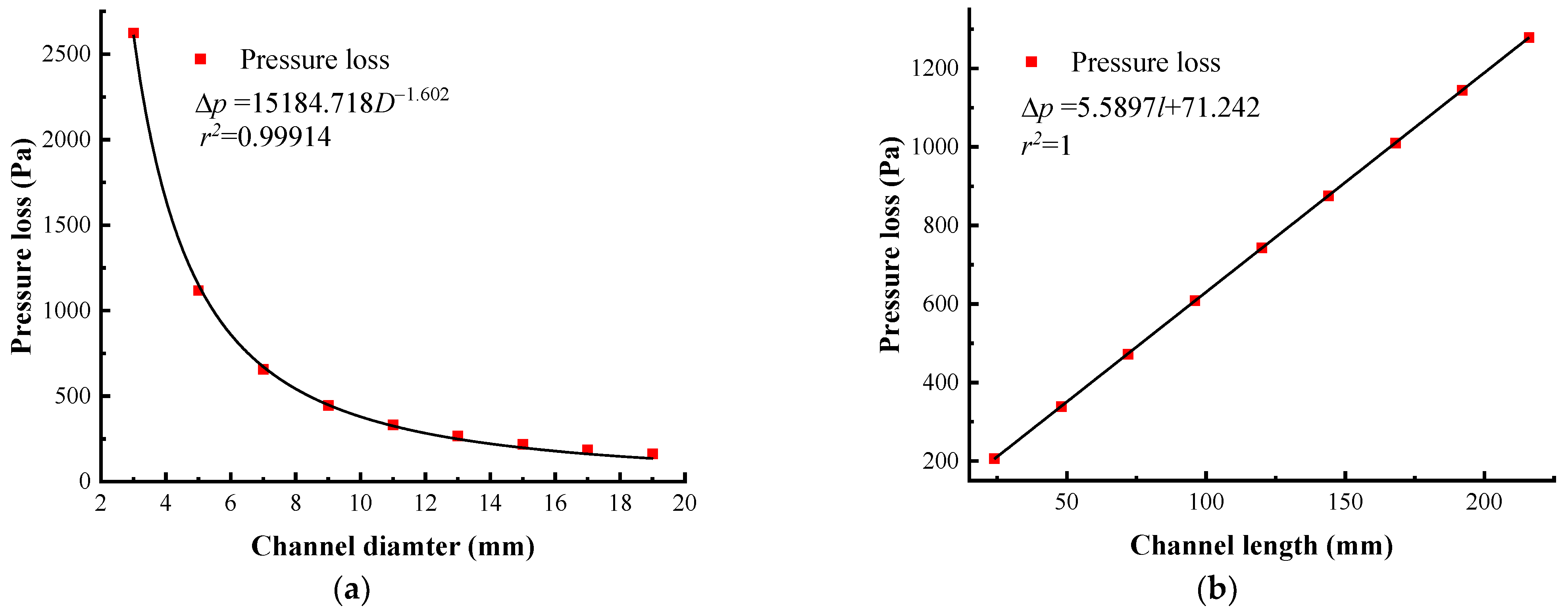
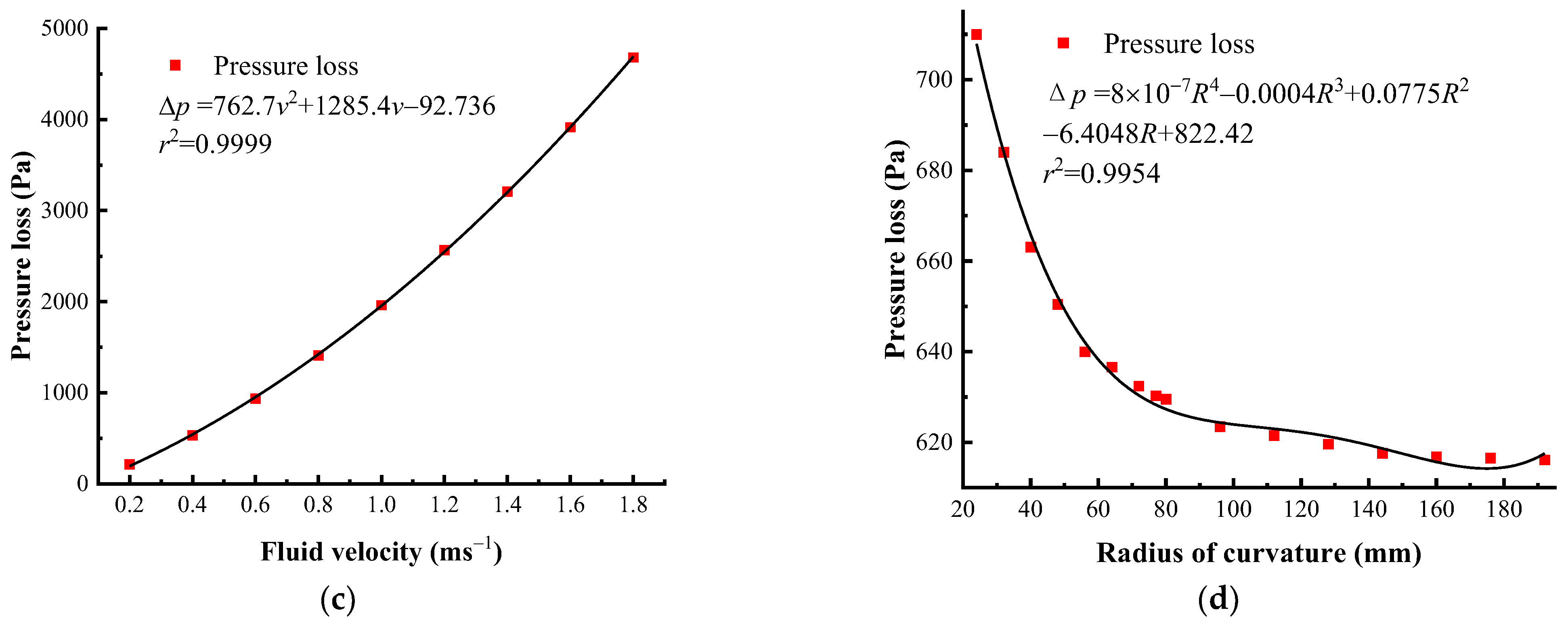
  • Within the range of the hydraulic valve flow channel size, the relationship between the flow channel diameter and the pressure loss was a quadratic function, and the pressure loss decreased with the increase in the flow channel diameter. The relationship between the length of the flow channel and the pressure loss was a linear function, and the pressure loss increased with the increase in the length of the flow channel. The relationship between fluid velocity and pressure loss was a quadratic function, and the pressure loss increased with the increase in fluid velocity. The relationship between the curvature radius and the pressure loss was a quadratic function, and the pressure loss decreased with the increase in the curvature radius. If R/D > 11, the change in the curvature radius had little effect on the pressure loss.
  • The fluid velocity had the greatest effect on the pressure loss in curved flow channels, followed by the flow channel diameter and flow channel length, and the flow channel curvature radius had the least effect on the pressure loss.
  • The mathematical model of pressure loss developed based on CFD simulation results and multiple regression analysis can be applied in the prediction of pressure loss at the stage of aviation hydraulic flow channels’ structural design.

Author Contributions

D.L.: writing—original draft, designing and realizing the experiments and numerical analysis; N.D. and H.W.: writing—review and editing, supervision; N.D.: funding acquisition; F.Z.: helping with the experiments. All authors have read and agreed to the published version of the manuscript.

Funding

The work was funded by the National Natural Science Foundation of China (under Grant No. 52275255).

Data Availability Statement

The data that support the findings of this study are available from the corresponding author, [author initials], upon reasonable request.

Conflicts of Interest

The authors declare no conflict of interest.

Appendix A

This section gives the detailed derivation process of Equations (4) and (7).
Detailed derivation process of Equation (4):
Δ m a = p Δ A ( p + Δ p ) Δ A Δ m g cos θ τ π Δ d Δ l
Due to
Δ m = ρ Δ l Δ A ,   cos θ = Δ z / Δ l ,   Δ A = π Δ d 2 4 ,
then:
Δ p = ( ρ Δ l a + ρ Δ z g + 4 τ Δ l Δ d )
τ = μ d v d ( Δ d )
when Δ l l , Δ d D , then:
Δ p = ( ρ l d d t ( d ( α R ) d t ) + ρ Δ z g + 4 μ l D d v d D )
Detailed derivation process of Equation (7):
M L 1 T 2 = L a 1 L a 2 L a 4 ( L T 1 ) a 3 ( M L 3 ) a 5 ( M L 1 T 1 ) a 6
Take the indexes a 1 , a 4 and a 6 as the undetermined coefficients.
a 5 + a 6 = 1 a 1 + a 2 + a 4 + a 3 3 a 5 a 6 = 1 a 3 a 6 = 2
We can know:
a 5 = 1 a 6 a 3 = 2 a 6 a 2 = a 1 a 4 a 6
Substitute into Equation (5):
Δ p = k l a 1 D a 2 v a 3 R a 4 ρ a 5 μ a 6
The following can be obtained:
Δ p = k ( l D ) a 1 ( R D ) a 4 ( μ ρ v D ) a 6 ρ v 2
Simplification:
Δ p = k ( L D ) a 1 ( R D ) a 4 ( 1 R e ) a 6 ρ v 2

References

  1. Campbell, I.; Bourell, D.; Gibson, I. Additive manufacturing: Rapid prototyping comes of age. Rapid Prototyp. J. 2012, 18, 255–258. [Google Scholar] [CrossRef]
  2. Liu, G.; Zhang, J.H.; Xu, B. Structure optimization for passages in hydraulic manifolds using metal additive manufacturing technology. In Proceedings of the 2019 IEEE 8th International Conference on Fluid Power and Mechatronics, Wuhan, China, 10–13 April 2019. [Google Scholar]
  3. Guo, N.; Leu, M.C. Additive manufacturing: Technology, applications and research needs. Mech. Eng. 2013, 8, 215–243. [Google Scholar] [CrossRef]
  4. Yang, S.; Zhao, Y.F. Additive manufacturing-enabled design theory and methodology: A critical review. Int. J. Adv. Manuf. Technol. 2015, 80, 27–342. [Google Scholar] [CrossRef]
  5. Thompson, M.K.; Moroni, G.; Vaneker, T.; Fadel, G.; Campbell, R.I.; Gibson, I.; Bernard, A.; Schulz, J.; Graf, P.; Ahuja, B. Design for additive manufacturing: Trends, opportunities, considerations, and constraints. CIRP Ann. 2016, 65, 737–760. [Google Scholar] [CrossRef]
  6. Pavel, R.; Leonid, R.; Ivan, S. Analysis of hydraulic units manufactured by powder bed fusion. In Proceedings of the 2018 Global Fluid Power Society PHD Symposium, Samara, Russia, 18–20 July 2018. [Google Scholar]
  7. Paolini, A.; Kollmannsberger, S.; Rank, E. Additive manufacturing in construction: A review on processes, applications, and digital planning methods. Addit. Manuf. 2019, 30, 100894. [Google Scholar] [CrossRef]
  8. Ngo, T.D.; Kashani, A.; Imbalzano, G.; Nguyen, K.T.Q.; Hui, D. Additive manufacturing (3D printing): A review of materials, methods, applications and challenges. Compos. Part B Eng. 2018, 143, 172–196. [Google Scholar] [CrossRef]
  9. Oh, Y.; Zhou, C.; Behdad, S. Part decomposition and assembly-based (Re) design for additive manufacturing: A review. Addit. Manuf. 2018, 22, 230–242. [Google Scholar] [CrossRef]
  10. Chen, L.; He, Y.; Yang, Y.X.; Niu, S.W.; Ren, H.T. The research status and development trend of additive manufacturing technology. Int. J. Adv. Manuf. Technol. 2017, 89, 3651–3660. [Google Scholar] [CrossRef]
  11. Gisario, A.; Kazarian, M.; Martina, F.; Mehrpouya, M. Metal additive manufacturing in the commercial aviation industry: A review. J. Manuf. Syst. 2019, 53, 124–149. [Google Scholar] [CrossRef]
  12. Fasel, U.; Keidel, D.; Baumann, L.; Cavolina, G.; Eichenhofer, M.; Ermanni, P. Composite additive manufacturing of morphing aerospace structures. Manuf. Lett. 2020, 23, 85–88. [Google Scholar] [CrossRef]
  13. Segonds, F. Design by additive nanufacturing: An application in aeronautics and defence. Virtual Phys. Prototyp. 2018, 13, 237–245. [Google Scholar] [CrossRef]
  14. Joyee, E.B.; Pan, Y.Y. Additive manufacturing of multi-material soft robot for on-demand drug delivery applications. J. Manuf. Process. 2020, 56, 1178–1184. [Google Scholar] [CrossRef]
  15. Culmone, C.; Smit, G.; Breedveld, P. Additive manufacturing of medical instruments: A state-of-the-art review. Addit. Manuf. 2019, 27, 461–473. [Google Scholar] [CrossRef]
  16. Zhang, C.; Wang, S.; Li, J.; Zhu, Y.; Peng, T.; Yang, H.Y. Additive manufacturing of products with functional fluid channels: A review. Addit. Manuf. 2020, 36, 1101490. [Google Scholar] [CrossRef]
  17. Biedermann, M.; Beutler, P.; Mirko, M. Automated design of additive manufactured flow components with consideration of overhang constraint. Addit. Manuf. 2021, 46, 102119. [Google Scholar] [CrossRef]
  18. Schmelzle, J.; Kline, E.V.; Dickman, C.J.; Reutzel, E.W.; Jones, G.; Simpson, T.W. (Re)Designing for part consolidation: Understanding the challenges of metal additive manufacturing. J. Mech. Des. 2015, 137, 111404. [Google Scholar] [CrossRef]
  19. Diegel, O.; Schutte, J.; Ferreira, A.; Chan, Y.L. Design for additive manufacturing process for a lightweight hydraulic manifold. Addit. Manuf. 2020, 36, 101446. [Google Scholar] [CrossRef]
  20. Chekurov, S.; Lantela, T. Selective laser melted digital hydraulic valve system. 3D Print. Addit. Manuf. 2017, 4, 215–221. [Google Scholar] [CrossRef]
  21. Aiman, A.A.; Calzone, F.; Muzzupappa, M. Hydraulic manifold design via additive manufacturing optimized with CFD and fluid structure interaction simulations. Rapid Prototyp. J. 2018, 25, 1516–1524. [Google Scholar]
  22. Cooper, D.E.; Stanford, M.; Kibble, K.A.; Gibbons, G.J. Additive manufacturing for product improvement at Red Bull Technology. Mater. Des. 2012, 41, 226–230. [Google Scholar] [CrossRef]
  23. Zardin, B.; Cillo, G.; Rinaldini, C.A.; Mattarelli, E.; Borghi, M. Pressure losses in hydraulic manifolds. Energies 2017, 10, 310. [Google Scholar] [CrossRef] [Green Version]
  24. Zardin, B.; Cillo, G.; Borghi, M.; D’Adamo, A.; Fontanesi, S. Pressure losses in multiple-elbow paths and in V-bends of hydraulic manifolds. Energies 2017, 10, 788. [Google Scholar] [CrossRef]
  25. Zhang, J.H.; Liu, G.; Ding, R.Q.; Zhang, K.; Pan, M.; Liu, S.H. 3D printing for energy-saving: Evidence from hydraulic manifolds design. Energies 2019, 12, 2462. [Google Scholar] [CrossRef]
  26. Zhang, H.; Zhang, X.X.; Sun, H.S.; Chen, M.J.; Lu, X.Y.; Wang, Y.C.; Liu, X.T. Pressure of newtonian fluid flow through curved pipes and elbows. J. Therm. Sci. 2013, 22, 372–376. [Google Scholar] [CrossRef]
  27. Da Silva, R.P.P.; Mortean, M.V.V.; de Paiva, K.V.; Beckedorff, L.E.; Oliveira, J.L.G.; Brandao, F.G.; Monteiro, A.S.; Carvalho, C.S.; Oliveira, H.R.; Borges, D.G.; et al. Thermal and hydrodynamic analysis of a compact heat exchanger produced by additive manufacturing. Appl. Therm. Eng. 2021, 193, 116973. [Google Scholar] [CrossRef]
  28. Tang, W.B.; Xu, G.S.; Zhang, S.J.; Jin, S.F.; Wang, R.X. Digital Twin-Driven Mating Performance Analysis for Precision Spool Valve. Machines 2021, 9, 157. [Google Scholar] [CrossRef]
  29. Li, D.F.; Dai, N.; Wang, H.T. Optimization design of hydraulic valve block and its internal flow channel based on additive manufacturing. Trans. Nanjing Univ. Aeronaut. Astronaut. 2021, 38, 373–382. [Google Scholar]
  30. Li, A.H.; Lan, Q.Q.; Dong, D.S.; Liu, Z.; Li, Z.Z.; Bian, Y.M. Integrated design and process analysis of a blow molding turbo-charged pipe. Int. J. Adv. Manuf. Technol. 2014, 73, 63–72. [Google Scholar] [CrossRef]
  31. Asztalos, Z.; Szava, I.; Vlase, S.; Szava, R.I. Modern dimensional analysis involved in polymers additive manufacturing optimization. Polymers 2022, 14, 3995. [Google Scholar] [CrossRef]
  32. Chen, X.D.; Nie, G.J.; Wu, Z.M. Global buckling and wrinkling of variable angle tow composite sandwich plates by a modified extended high-order sandwich plate theory. Compos. Struct. 2022, 292, 115639. [Google Scholar] [CrossRef]
  33. Favero, G.; Berti, G.; Bonesso, M.; Morrone, D.; Oriolo, S.; Rebesan, P.; Dima, R.; Gregori, P.; Pepato, A.; Scanavini, A.; et al. Experimental and numerical analyses of fluid flow inside additively manufactured and smoothed cooling channels. Int. Commun. Heat Mass 2022, 135, 106128. [Google Scholar] [CrossRef]
  34. Gong, G.H.; Ye, J.J.; Chi, Y.M.; Zhao, Z.H.; Wang, Z.F.; Xia, G.; Du, X.Y.; Tian, H.F.; Yu, H.J.; Chen, C.Z. Research status of laser additive manufacturing for metal: A review. J. Mater. Res. Technol. 2021, 15, 855–884. [Google Scholar] [CrossRef]
  35. Favero, G.; Bonesso, M.; Rebesan, P.; Dima, R.; Pepato, A.; Mancin, S. Additive manufacturing for thermal management applications: From experimental results to numerical modeling. Int. J. Thermofluids 2021, 10, 100091. [Google Scholar] [CrossRef]
  36. Farwaha, H.S.; Deepak, D.; Brar, G.S. Design and performance of ultrasonic assisted magnetic abrasive finishing combined with electrolytic process set up for machining and finishing of 316L stainless steel. Mater. Today 2020, 33, 1626–1631. [Google Scholar]
Figure 1. Three-dimensional space flow channel composed of different curvature radii.
Energies 16 01788 g001
Figure 3. Experiment preparation: (a) flow channel samples fabricated using selective laser melting (SLM); (b) electrochemical polishing schematic.
Energies 16 01788 g003
Figure 4. (a) A schematic of the pressure loss test rig; (b) a photo showing the test rig.
Energies 16 01788 g004
Figure 5. Relationship curve between pressure loss ( Δ p ) and flow channel design parameters: (a) relationship curve between D and Δ p ; (b) relationship curve between l and Δ p ; (c) relationship curve between v and Δ p ; (d) relationship curve between R and Δ p .
Energies 16 01788 g005aEnergies 16 01788 g005b
Figure 6. Correction curve for the relationship between curvature radius and pressure loss: (a) relationship curve between R and Δ p (R/D ≤ 11); (b) relationship curve between R and Δ p (R/D > 11).
Energies 16 01788 g006
Figure 7. (a) Comparison of pressure loss simulation and calculation results; (b) comparison of pressure loss test and calculation results.
Energies 16 01788 g007
Figure 8. Test results and mathematical model calculation results of the fluid velocity variation in SLM-fabricated flow channel samples.
Energies 16 01788 g008
Table 1. Simulation results of pressure loss for mesh with different sizes.
Mesh Size (mm)Number of Mesh ElementsPressure Loss (Pa)
0.19,613,0001497.8
0.21,460,5001497.4
0.3494,5051469.3
0.4224,7501413.4
Table 2. Flow channel design parameters and their corresponding values with levels.
SymbolsParametersLevelsUnits
1234
lFlow channel length70100130160mm
vFluid velocity0.51.52.53.5ms−1
RCurvature radius406080100mm
DFlow channel diameter691215mm
Table 3. Simulation results of orthogonal experimental design.
Experiment Number l v (ms−1)R (mm)D (mm)EmptyPressure Loss (Pa)
1701.5801221262.7
21003.540927449.8
31303.5801535076.8
41601.540636355.1
5702.5401542336.4
61000.58064981.1
71300.540121504.2
81602.580916917.1
9700.510093385.8
101002.5601234584.8
111302.5100629002
121600.560152431.5
13703.560617838.9
141001.51001511267.8
151301.560943073.3
161603.51001247386.1
Table 4. The structural and experimental parameters of the flow channel samples.
Sample Number l v (ms−1)R (mm)D (mm)
11002.5809
21602.510012
3703.56012
41301.58012
5701.51009
61003.51006
71001.56015
81603.58015
Table 5. Pressure loss ( Δ p ) range analysis.
l vRDEmpty
K12955.95575.654161.3756044.2754132
K23570.8752989.7253982.1254456.54536.5
K34414.0755710.0753559.4253434.454100.625
K45272.456937.94510.4252278.1253444.225
Range2316.56362.259513766.151092.275
Rank31524
Table 6. Orthogonal experimental simulation results and mathematical model calculation results.
Experiment Number l v (ms−1)R (mm)D (mm)SimulationCalculationError
Pressure Loss (Pa)Pressure Loss (Pa)(%)
11002.58094504.14589.51.89
21600.56091213.211642.535.38
31602.5100124786.85110.86.76
41000.54012408.6455.511.47
51300.510015388.2442.714.03
6702.540151840.11840.40.016
7700.5806807.61136.840.76
81302.56068361.98590.72.73
9703.560124134.34063.11.72
101301.580122072.32259.59.03
111303.54098713.18830.71.34
12701.510091659.61780.67.29
131601.54065964.25993.90.49
141003.5100610,534.910,685.41.42
151001.560151348.61224.39.21
161603.580156019.16350.75.5
Table 7. Comparison between the test results of the flow channel samples and the calculation results of the mathematical model.
Sample NumberCalculation Results (Pa)Test Results (Pa)Error (%)
14589.4548515.69
25110.844992.52.31
34063.0942238.85
42259.51147.70.52
51780.6218554.12
610,685.410,214.44.4
71224.321473.120.31
86350.76244.61.67
Table 8. Comparison between the test results of the flow channel samples and the calculation results of the mathematical model.
Fluid Velocity
(ms−1)
Calculation Results
(Pa)
Test Results
(Pa)
Error
(%)
Calculation Results
(Pa)
Test Results
(Pa)
Error
(%)
Calculation Results
(Pa)
Test Results
(Pa)
Error
(%)
Calculation Results
(Pa)
Test Results
(Pa)
Error
(%)
0.51685.911875.211.22496.55508.32.361054.291189.312.81196.12321.563.93
0.752194.432430.710.76780.78823.75.491443.711514.34.89423.7542.728.08
12746.852928.16.591089.5511646.831866.731987.36.45670.9274511.04
1.253343.173566.66.681422.861508.76.032323.382417.34.04937.791023.29.1
1.53983.394002.30.471780.701855.34.182813.642948.94.81224.3113248.14
1.754667.514757.41.922163.082282.45.513337.523482.24.331530.471685.410.12
25395.525302.21.7225702688.14.593895.013979.12.161856.271976.56.47
2.256167.436216.80.83001.4531224.014486.124601.22.562201.732342.16.37
2.56983.256859.11.773457.443557.22.885110.844992.42.312566.822741.36.79
No. 6 sample D = 6 mmNo. 5 sample D = 9 mmNo. 2 sample D = 12 mmNo. 7 sample D = 15 mm
Disclaimer/Publisher’s Note: The statements, opinions and data contained in all publications are solely those of the individual author(s) and contributor(s) and not of MDPI and/or the editor(s). MDPI and/or the editor(s) disclaim responsibility for any injury to people or property resulting from any ideas, methods, instructions or products referred to in the content.

