Article

Thin Reservoir Identification Based on Logging Interpretation by Using the Support Vector Machine Method

1
Research Institute of Petroleum Exploration and Development, China National Petroleum Corporation, Beijing 100083, China
2
College of Geosciences, China University of Petroleum-Beijing, Beijing 102249, China
3
School of Geosciences, Yangtze University, Wuhan 430100, China
*
Author to whom correspondence should be addressed.
Energies 2023, 16(4), 1638; https://doi.org/10.3390/en16041638
Submission received: 23 December 2022 / Revised: 30 January 2023 / Accepted: 31 January 2023 / Published: 7 February 2023

Abstract

:
A reservoir with a thickness less than 0.5 m is generally considered to be a thin reservoir, in which it is difficult to directly identify oil-water layers with conventional logging data, and the identify result coincidence rate is low. Therefore, a support vector machine method (SVM) is introduced in the field of oil-water-dry layer identification. The basic approach is to map the nonlinear problem (input space) to a new high-dimensional feature space through the introduction of a kernel function, and then construct the optimal decision surface in the high-dimensional feature space and conduct sample classification. There are plenty of thin reservoirs in Wangguantun oilfield. Therefore, 63 samples are established by integrating general logging data and oil testing data from the study area, including 42 learning samples and 21 prediction samples, which are normalized. Then, the kernel function is selected, based on previous experience, and the fluid identification model of the thin reservoir is built. The model is used to identify 21 prediction samples; 18 are correct, and the prediction accuracy reaches 85.7%. The results show that the SVM method is feasible for fluid identification in thin reservoirs.

1. Introduction

The oil fields previously developed in China are now entering the “double extra-high” development stage, with a high water cut and a high recovery degree, and the oil field output continues to decline. In the early stages of development, the main oil layer con-tributes to the main output of the reservoir, while the thin oil layer is labeled as “poor physical property” and “poor production” due to its own physical conditions [1], and is often not given priority in a development plan. In order to ensure the stable production of old oilfield areas, many oil fields transfer to explore potential objects and change the development mode. The potential of non-major oil reservoirs, such as thin and differential oil reservoirs, cannot be ignored [2,3,4]. For example, the proven geological reserves of medium-thin and low-margin oil reservoirs in Sazhong Development Zone of Daqing Changyuan are more than 300 million tons, accounting for 2/5 of the total geological reserves. The exploitation and utilization of the medium-thin and low-margin oil reservoirs have contributed to the production of Changyuan and provided a guiding direction for the production growth of old block. The exploitation and utilization of the medium-thin and low-margin oil reservoirs have contributed to the production of Changyuan and provided a guiding direction for the production growth of old block.
This paper takes the thin oil layer of the third member of the Shahejie Formation in the Guan187 area as the research object. The main oil-producing reservoirs in the Guan187 area are the first member of the Shahejie Formation and the third member of the Shahejie Formation of Paleogene. In recent years, the water content of the block has been high and liquid production has been low, and most of the oil wells have been shut down at low energy. There are a lot of potential reservoirs in the three oil formations of the third member of the Shahejie Formation, which can be interpreted as a dry reservoir, a low yield reservoir, and a poor oil reservoir, which are suitable for the research aim of this paper. In this paper, the identification method of a thin differential reservoir is established by comprehensively using various logging curves. This research can play a key role in the future development of unutilized reserves of similar reservoirs.
For most thin oil layers, the 2.5 m and 4.4 m apparent resistivity and spontaneous potential charts can distinguish between oil and water layers. Liu Jiang [5] adopted the conventional identification method to establish the four relationships between the oil layer, the water layer, and the dry layer, to establish the interpretation template, determine the lower limit value of thin differential oil layer, and identify it. The identification results have a high coincidence rate. Guo Hongyan [6] proposed an effective method for the fluid identification of thin differential reservoirs. Carbon-oxygen ratio energy spectrum logging was used to improve the interpretation accuracy of thin differential reservoirs. The interpretation chart was drawn combined with spontaneous potential, and the interpretation results were highly consistent with the oil test results. Shan Xuguang [7] used the Fourier spectrum method, the resolution matching method, and other methods for comparative processing to improve the resolution of thin layer identification, more accurately restore the real logging value of thin oil layer, and make the prediction results more in line with reality. Tang Hong [8] used variance functions to correct logging curves, improve logging identification resolution, and accurately interpret thin differential oil formations. Hou Jun [9] used wave impedance inversion to simulate the deep lateral resistivity prediction reservoir sand body and effectively identify the thin sand body with a thickness of 0.5 m.
For thin reservoirs, the logging response value of the target layer is greatly affected by the surrounding rock. It is difficult to quantitatively identify oil and water layers by conventional logging interpretation methods. Under the conditions of very limited sample data, it is necessary to seek a method that can integrate various logging and geological information to identify oil and water. Because the lithology of the reservoir is complex, its shale content is high, and the reservoir is mainly thin interbedded, resulting in the logging response being distorted and affected to different degrees. The identification of oil and water layers is difficult, the log interpretation coincidence rate is low, and the traditional empirical log interpretation is gradually unable to meet the production needs. Therefore, this paper proposes the artificial intelligence method of support vector machine (SVM) to identify thin layers.
Support vector machine (SVM) is a machine learning algorithm proposed by VAPNIK in the mid 1990s [10,11]. It is a pattern classifier based on VC dimension theory of statistical learning theory and structural risk minimization principle [12]. It has the advantages of complete theory, strong adaptability, global optimization, a short training time, and great generalization performance. It can successfully solve the “dimensionality disaster” problem in traditional learning methods, and has been widely used in pattern recognition, regression estimation, reservoir prediction, and other fields, which are research hotspots in the field of machine learning.

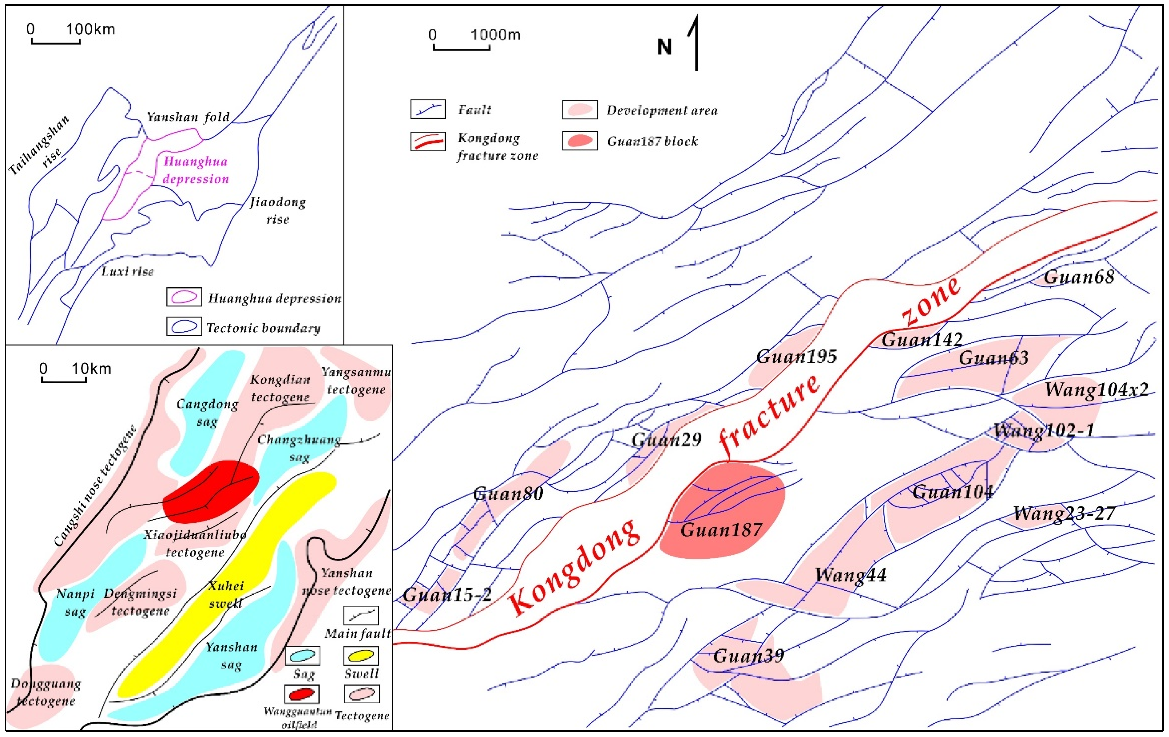
2. Overview of Research Area

The study area is Guan187 area in Wangguantun oilfield, south area of Huanghua Depression. Huanghua Depression is located in the central part of Bohai Bay Basin with a total area of 1.7 × 10⁴ km2. It is adjacent to Yanshan Fold in the north, Cangxian Uplift in the west, and Chengning Uplift and Bozhong Depression in the southeast. It is spread in a long strip in the direction of NEE-SW, and the width of the depression is up to 70 km. Wangguantun oilfield is located on the Kongdian tectonic belt in the southern area of the Huanghua Depression, and is divided into two parts by the Kongdong fault zone [13,14,15]. It is adjacent to Cangdong Depression in the north, the Liupu tectonic belt in the Xiaoji fault in the south, and the Changzhuang Depression in the east. The Guan187 area is located in the middle of Wangguantun oilfield and is on the east side of the Kongdong fault zone. It contains two major development fault blocks, Guan187 and Guan913, with an area of about 9.6 km2 (Figure 1 and Figure 2). Among them, the third member of Shasan-3 contains a large number of non-major formations, such as low-producing and thin oil formations, which are the main research objects of this paper.
Located in the east of the Kongdong fault zone and controlled by the Kongdong fault, the Guan187 area is high in the north and low in the south, and its interior is divided by several faults [16,17]. The whole study area is divided into the northern Guan187 fault block and the southern Guan913 fault block by the central fault. The highest point of the structure in the whole area is near well G187, which gradually decreases to the four sides, forming an anticlinal trap. There is a secondary high near Wang 34-2, which gradually decreases to the four sides (Figure 2).
The target horizon of this paper is the third oil formation of the third member of Shahejie Formation, which belongs to the Shahejie Formation. The lower strata are the Paleogene Kongdian Formation, and the upper strata are the Dongying Formation, Guantao Formation, and Minghuazhen Formation. In the Shahejie Formation, the lower part of the first member of the Shahejie Formation and the third member of the Shahejie Formation are the main oil-producing reservoirs in this area. The third member of the Shahejie Formation can be subdivided into three oil groups. Affected by paleotopography, strata in the study area show a trend of thickening in the south and thinning in the north, with large thicknesses in low parts and thin thicknesses in high parts as a whole. The thickness of sandstone in the reservoir also has a certain thinning trend. There are a large number of thin layers of light green fine sandstone and argillaceous siltstone in the third oil formation of the third member of the target formation, which are mainly characterized by “mud-coated sand”. The upper part of the Sha32 oil Formation contains a set of stable volcanic rock sedimentary layers, and the lower part of the Zao 0 oil Formation of the first member of the Kongdian Formation is lake deposition, with a set of stable paste rock layers. Therefore, the target interval can be accurately identified and divided. Most of the wells can be drilled into the third oil group of the third member of the Shahejie Formation. In some areas, due to the influence of the central fault, the target strata have a formation loss phenomenon to varying degrees (Table 1).

3. SVM Classification Principle
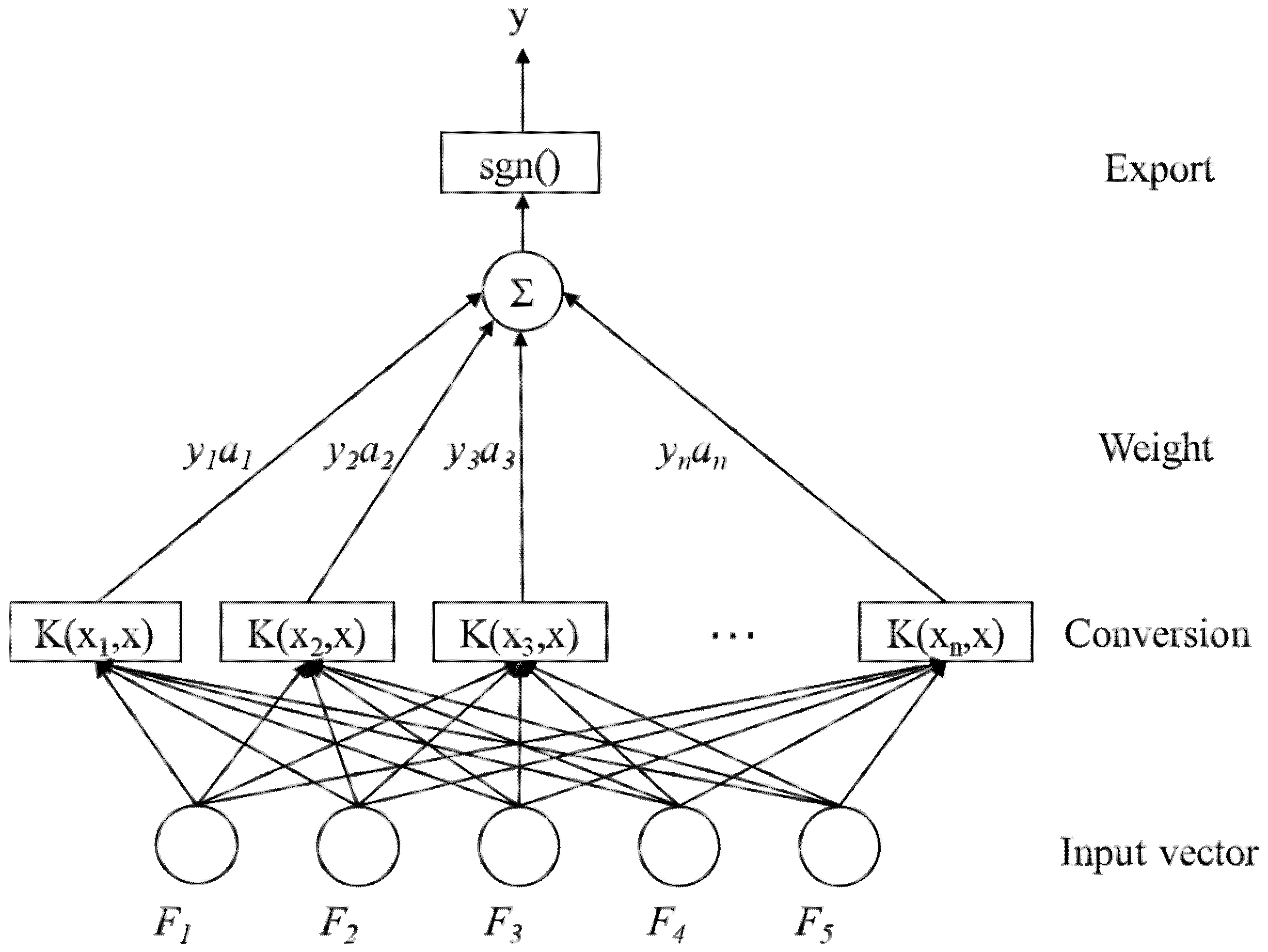
Support Vector Machine (SVM), first proposed by Vapnik, is a new machine learning method based on statistical theory [18]. The basic approach is to map the nonlinear problem (input space) to a new high-dimensional feature space by introducing a kernel function, and then construct the optimal decision surface in the high-dimensional feature space and conduct sample classification (Figure 3). Support vector machines (SVM) have the advantages of high accuracy, fast speeds, strong versatility, and perfect theory when solving nonlinear problems related to research targets and multiple uncertain features [19].
SVM’s core idea is that, for a given learning task with a limited number of training samples, there is a trade-off between the accuracy of the given training set and machine capacity with the preferable generalization capability [20]. Since the final solution of the SVM is a convex optimization problem, the obtained solution must be the global optimal solution, which is not found in other algorithms, including neural networks.
This paper uses the support vector machine (SVM) algorithm with strong nonlinear processing ability to classify and identify thin layers. The structure diagram of the support vector machine algorithm and the thin layer division process are shown in Figure 4 and Figure 5. The implementation process of the algorithm is as follows: the known samples are selected to form learning samples to train the model, so as to establish the thin layer quantitative recognition model; the prediction model is verified by the test samples; and the thin layer of unknown samples is predicted by the verified prediction model.

3.1. Two-Class SVM

Assume that sample set ( x i , y i ) , i = 1 , 2 , , n , x i R d , y i y = { + 1 , 1 } . For the case of a linearly separable sample set separated by a hyperplane. Remember the hyperplane w · x + b = 0 , where w is the normal line of the classification surface, b is the outlier that represents the position of the modified normal with respect to the origin [21]. The optimal hyperplane not only separates the two types of samples error-free, but also maximizes the classification interval. The problem of optimal hyperplane construction can be translated to calculate the minimum of the formula
{ φ ( w ) = 1 2 w 2 s , t , y i ( x i · w + b ) 1 i = 1 , 2 , , n
The problem can also be transformed into a simpler dual problem to calculate the maximum of the formula:
{ Q ( α ) = i = 1 n a i 1 2 i = 1 n j = 1 n α i α j y i y j ( x i · x j ) s , t , i = 1 n y i α i = 0 α i 0
where, α i is the Lagrange multiplier for each sample. According to the condition of Kuhn-Tucher, the optimal solution must satisfy the following conditions:
α i [ y i ( w · x i + b ) 1 ] = 0 i = 1 , 2 , , n
Therefore, only the support vector coefficients α i are a non-zero value. If α i is the optimal solution,
w * = i = 1 n α i * y i x i
By choosing the corresponding i when α i 0 , we can obtain the value of b using Formula (3). Then, the optimal classification function can be obtained by substituting w* and b into the formula sgn ( w * · x + b ) .
For a linearly inseparable case, we can introduce a slack vector ξ, which satisfies:
{ y i [ ( w · x i ) + b ] 1 ξ i ξ i 0 i = 1 , 2 , , n
The generalized optimal classification surface can be obtained by changing the objective to find the minimum value of formula φ ( w , ξ ) = 1 2 w 2 + C i = 1 n ξ i , where C stands for penalty function, it shows the penalty for misclassification.
For nonlinear problems, it can be transformed into a linear problem in a higher dimensional space by nonlinear transformation and obtain the optimal classification surface. The linear classification of a nonlinear problem after transformation can be realized by using the proper kernel function. In this case, the classification function named SVM is:
f ( x ) = sgn { α i * y i K ( x i , x ) + b * }
The function’s remarkable feature is that data only appear in the inner product. It is not necessary to know the specific nonlinear mapping process before calculation, only to select an appropriate model to replace the inner product, so as to economize the complex calculation. It should be noted that the model here must satisfy the conditional kernel parameters.

3.2. Multi-Class SVM

SVM technology was originally proposed for the two-class problem, but the oil-water-dry layer identification problem belongs to the multi-class problem. In order to effectively use the SVM method to divide the oil-water-dry layers, it is necessary to extend the SVM and build a reasonable multi-class coding scheme [22,23]. At present, there are two main methods for constructing SVM multi-class: one is the direct method, represented by the multi-class algorithm proposed by Weston [22], which has a high degree of complexity and is difficult to implement. The other is the indirect method, which mainly includes “one-to-one”, “one-to-many”, and a SVM decision tree. This paper mainly adopts the “one-to-one” method and uses the Libsvm classifier for training [24]. Libsvm is a simple, practical, fast, and effective SVM pattern recognition and regression software package. The algorithm combines the ideas of SMO and SVM-Light, and adopts a voting strategy to support multi-class. By training k(k − 1)/2 classifiers, the samples are labeled with the highest votes. The principle of the “one-to-one” algorithm is as follows: if there are k types of data, select the i-th type of data and the j-th type of data to construct a classifier, where i < j, so that k(k − 1)/2 classifiers need to be trained. For the i-th and j-th types of data, a two-class problem needs to be solved:
min w i j , b i j , ξ i j 1 2 ( w i j ) T w i j + C t ξ t i j
If y t = i ,
( w i j ) T φ ( x i ) + b i j 1 ξ t i j
If y t = j , ξ t i j 0 ,
( w i j ) T φ ( x i ) + b i j 1 + ξ t i j
Solve this problem by using the voting method: If sign [ ( w i j ) T , φ ( x i ) + b i j ] , consider x as the i-th type, i-th type plus one vote; else j-th type plus one vote. Finally, x belongs to the type with the most votes.

4. Application of SVM in Thin Reservoir Identification
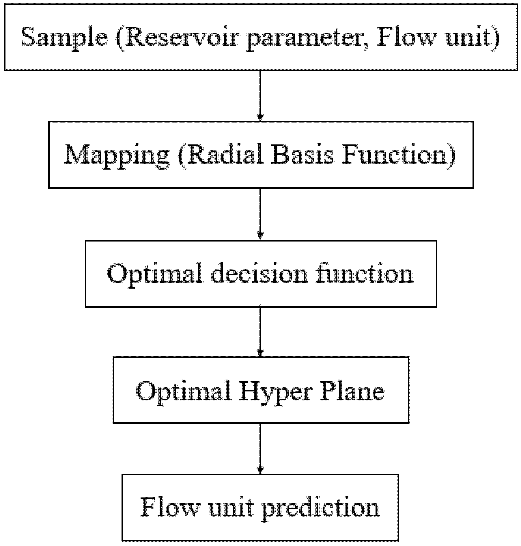
The identification of an oil layer, a water layer, and a dry layer belongs to the problem of multi-class discriminant pattern recognition, so it can be completed by using the SVM method to establish a fluid identification model. The basic idea is to collect modeling samples and perform data preprocessing to generate feature quantities first, and then perform parameter optimization to determine the best combination of parameters for modeling, and finally use the established model to predict targets and identify oil-water-dry layers.

4.1. Model Building

Model construction mainly includes the determination of the kernel function and penalty factor C. The most common kernel functions in SVM mainly include the Gaussian radial basis kernel function, the multi-layer perceptron kernel function, and the polynomial kernel function. In this section, the well logging curve is optimized, the sample points are collected, and then the kernel function is optimized to establish a model to identify the thin layer.

4.1.1. Sample Set Selection

The identification of an oil-water-dry layer is an important feature of logging evaluation. The logging curve indirectly reflects the properties of the fluid in the reservoir. Different logging curves will show a certain degree of difference and regularity for different fluid characteristics, such as oil-water-dry layers [25]. Through the description of logging characteristics, integrate the interpretation experience of experts and the correlation analysis and comparison of coring wells. Finally, we select the logging curves closely related to reservoir fluid, such as: acoustic (AC), true formation resistivity (RT), neutron (CNL), density (DEN), natural gamma ray (GR), spontaneous potential (SP); porosity (POR), used as input eigenvalues for the sample. The output positive integer represents the fluid identification result, where 1 represents the oil layer, 2 represents the water layer, and 3 represents the dry layer. By stratifying the logging curve and combining it with the oil test data, the typical characteristics of oil, water, and dry layers of seven wells were selected as the training objects and the remaining four wells were selected as the testing objects in the study area. Several reliable and representative logging data from each study interval were selected as training samples for this interval. Finally, a total of 203 logging data from 42 characteristic layers in seven wells were selected as the training sample dataset. According to the oil test data, the test sample dataset was obtained from the remaining four wells using a logging curve from twenty-one layers when building test samples.

4.1.2. Normalization of Sample Data

There is no standardized format data obtained from logging data. Therefore, the data should be normalized first [26] in order to avoid the difficulty of calculating the inner product of the kernel function caused by the difference of each parameter dimension and improve the prediction accuracy. This can avoid some eigenvalue ranges that are too large and other eigenvalue ranges that are too small, resulting in large numbers drowning the decimal.
The normalization formula adopted is: X = ( x x min ) / ( x max x min ) , where x is the actual logging value, xmax, xmin are the maximum and minimum values among all sampling points of the logging curve, X is the log value after normalization, X [ 0 , 1 ] . The training and test samples are located in the normalized interval, which ensures the reliability of the classification results [27,28,29].

4.1.3. Model Selection

The identification of oil, water, and dry layers belongs to the problem of multi-class discriminant pattern recognition. In theoretical analysis, the determination of the classification function is mainly the determination of the kernel function r and penalty coefficient C. These two parameters have great influence on the prediction results, and their reasonable determination directly affects the accuracy and generalization ability of the model. The Gaussian radial basis function (GRBF) is usually used to establish the identification model of reservoir fluid. The cross-validation method is used to optimize the C and r [30,31,32,33,34]. The Gaussian radial basis kernel function has a wide convergence domain, has a high applicability for a variety of sample cases, and has only one kernel parameter r. It has a high flexibility, is currently the most widely used and the best effect of the classification kernel function. Therefore, the Gaussian radial basis kernel function is used to build the prediction model of support vector machine. The Gaussian radial basis kernel function formula is:
K ( x i , x ) = exp x x i 2 r 2
Finally, the optimal parameter combination is calculated as C = 4.1541 and r = 0.7218.

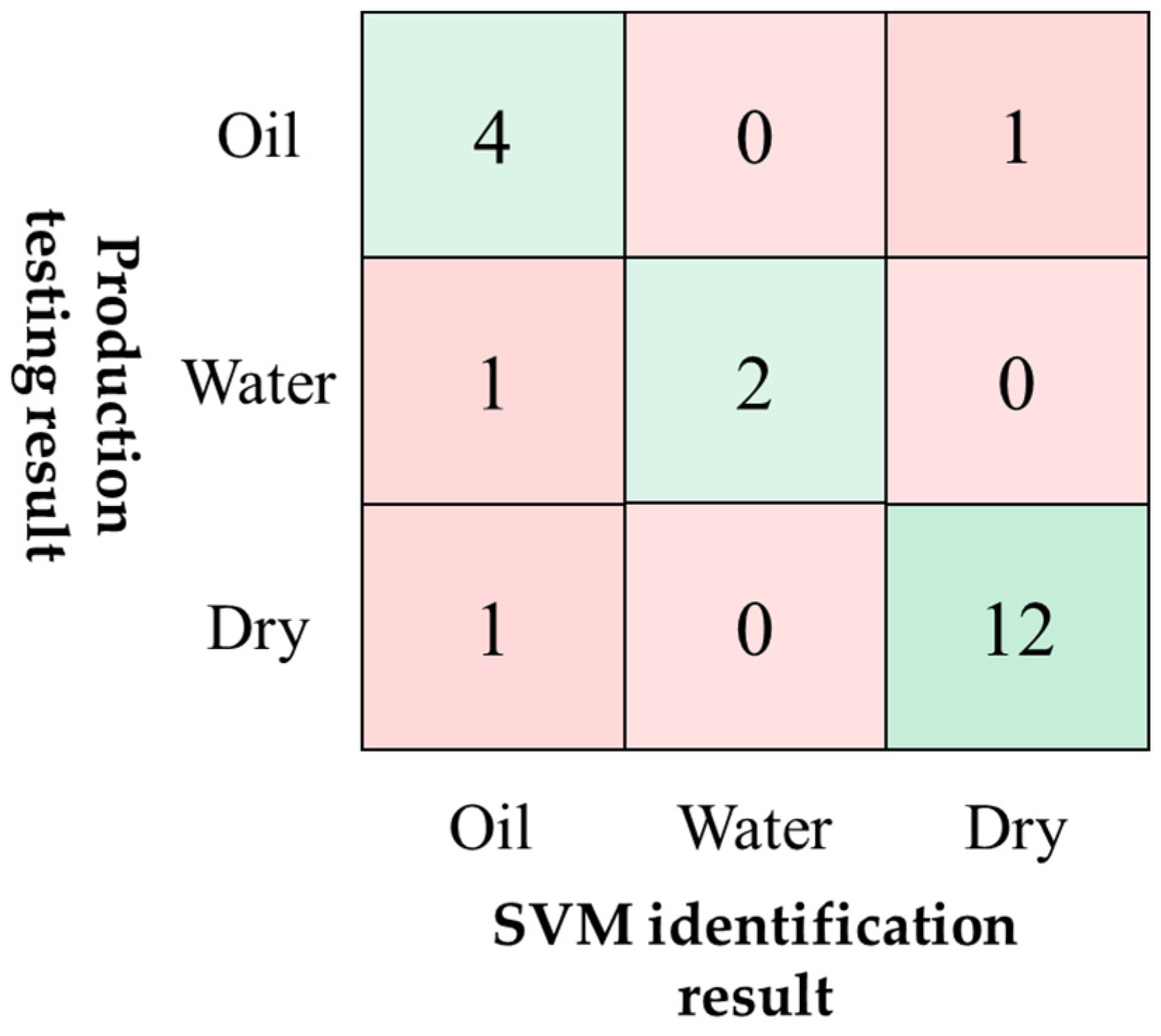
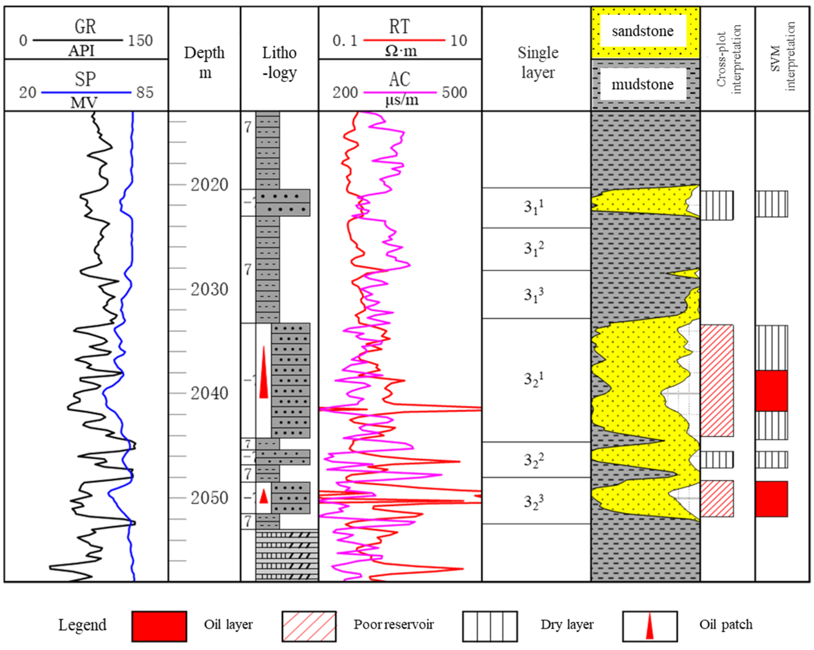
4.2. Application Effect and Analysis

Using MATLAB R2019a software, with forty-two logging data of eight single layers in seven wells of Wangguantun oilfield as training samples, the SVM model for identifying oil-water-dry layers in this area was established. The model was used to identify twenty-one layers in four other wells in the area. Finally, the identification results of inspection with the production testing results were compared, where 18 of the 21 layers were correctly identified; recognition accuracy was 85.71% (Figure 6), which was better than conventional cross-plot identification results at 80.95% (Figure 7).
In order to evaluate the reliability of the SVM method for layers fluid identification, the identified results were compared with the cross-plot method. The comparison results are shown in Table 2. Through comparison and analysis, the SVM method has the highest accuracy (85.71%) in identifying oil-water-dry layers, which is higher than the cross-plot identification accuracy (80.95%). The identification results show that the SVM method based on the principle of structural risk minimization has a more stable performance when solving thin reservoirs and small sample problems.
The method was applied to other wells in the study area to identify thin layer fluids, and well G9-14-4 was used as an example (Figure 8).

5. Conclusions

(1)
The logging curves indirectly reflect the properties of the fluid in the reservoir. Well log data can be used to comprehensively identify the thin layers.
(2)
The accuracy of the SVM method for reservoir fluid identification is obviously higher than that of the conventional cross-plot identification method.
(3)
The SVM-based reservoir fluid identification model has high convergence accuracy and strong generalization ability, and can make full use of limited logging data information to obtain the optimal identification results. Especially in areas where the test data are lacking or the oil-water system is complex, this method can improve the identification accuracy of the oil-water dry layer. It has good reference values in actual logging reservoir evaluation and can be extended to lithology identification and reservoir parameter prediction.

Author Contributions

X.Z.: Writing—original draft; Y.L.: Data curation; X.S.: Writing—review and editing; L.J.: Methodology; X.W.: Visualization. All authors have read and agreed to the published version of the manuscript.

Funding

This research was funded by Science Foundation of China University of Petroleum, Beijing, grant number 2462020YXZZ022 and CNPC Innovation Found (2021DQ02-0106).

Data Availability Statement

The data that support the findings of this study are available on request from the corresponding author.

Conflicts of Interest

The authors declare no conflict of interest.

References

  1. Yu, H. Study on remaining oil in the north of Daqing Oilfield. Acta Pet. Sin. 1993, 14, 72–80. [Google Scholar]
  2. Qadri, S.T.; Ahmed, W.; Haque, A.E.; Radwan, A.E.; Hakimi, M.H.; Abdel Aal, A.K. Murree Clay Problems and Water-Based Drilling Mud Optimization: A Case Study from the Kohat Basin in Northwestern Pakistan. Energies 2022, 15, 3424. [Google Scholar] [CrossRef]
  3. Haque, A.E.; Qadri, S.T.; Bhuiyan, M.A.H.; Navid, M.; Nabawy, B.S.; Hakimi, M.H.; Abd-El-Aal, A.K. Integrated wireline log and seismic attribute analysis for the reservoir evaluation: A case study of the Mount Messenger Formation in Kaimiro Field, Taranaki Basin, New Zealand. J. Nat. Gas Sci. Eng. 2022, 99, 104452. [Google Scholar] [CrossRef]
  4. Osinowo, O.O.; Ayorinde, J.O.; Nwankwo, C.P.; Ekeng, O.M.; Taiwo, O.B. Reservoir description and characterization of Eni field offshore Niger Delta, southern Nigeria. J. Pet. Explor. Prod. Technol. 2018, 8, 381–397. [Google Scholar] [CrossRef]
  5. Liu, J.; Wang, A.; Lang, F.; Zhang, J. A new technique for identifying the fliud in thin, poor and low resistivity pay zone. Well Logging Technol. 2000, 24, 515–517. [Google Scholar]
  6. Guo, H.; Huang, D.; Pan, G. Fluid identification and interpretation method of thin differential oil-water layer in low permeability reservoir. China Pet. Explor. 2001, 6, 31–33. [Google Scholar]
  7. Shan, X. The Research to Log Recognition Technology for Thin Oil Layer in Qilicun Oilfield. Bachelor’s Thesis, Xi’an Shiyou University, Xi’an, China, 2014; pp. 34–54. [Google Scholar]
  8. Tang, H.; Luo, M.; Yan, Q. Recognition and interpretation of water encroaching in thin and poor-quality pay zone. J. Southwest Pet. Inst. 2003, 25, 1–3. [Google Scholar]
  9. Hou, J.; Wang, J.; Wang, C.; Cheng, L. Application of thin & poor reservoir predicted technology to the Punan oilfield. Southwest Pet. Inst. 2006, 28, 53–56. [Google Scholar]
  10. Vapnik, V.N. The Nature of Statistical Learning Theory; Springer: New York, NY, USA, 1995; pp. 54–96. [Google Scholar]
  11. Luo, N. A New Method in Data Mining-Support Vector Machine. Softw. Guide 2008, 7, 30–31. [Google Scholar]
  12. Vapnik, V.; Levin, E.; Le, C.Y. Measuring the VC-Dimension of a Learning Machine. Neural Comput. 1994, 6, 851–876. [Google Scholar] [CrossRef]
  13. Yang, C. Genesis and accumulation of non-type natural gases in Huanghua depression, Dagang oilfield. Pet. Explor. Dev. 2006, 33, 335–339. [Google Scholar]
  14. Xia, R.; Tang, J. The development and evaluated patterns of Ordovician palaeo karst in the Huanghua depression. Pet. Explor. Dev. 2004, 31, 51–53. [Google Scholar]
  15. Jiao, Q.; Hou, J.; Xing, H. Anastomosing river sediment of the Zao 0 reservoir group in the Duanliubo oilfield, Huanghua depression. Pet. Explor. Dev. 2004, 31, 72–74. [Google Scholar]
  16. Ren, W. Fault structure characteristics of Guan-3 block in Wangguantun Oilfield. Petrochem. Ind. Technol. 2017, 8, 127. [Google Scholar]
  17. Zhang, X.; Hou, J.; Hu, C.; Liu, Y.; Wang, X.; Ji, L. Evaluation of reservoir permeability heterogeneity by principal component analysis—Taking Wangguantun oil field Wang 23–27 block for example. J. East China Univ. Technol. Nat. Sci. 2018, 41, 41–45. [Google Scholar]
  18. Vapnik, V.N. The Nature of Statistical Learning Theory, 2nd ed.; Springer: New York, NY, USA, 1999; pp. 12–15. [Google Scholar]
  19. Lu, W.; Guo, J.; Dong, H.; Zhang, Y.; Lin, L. Evaluating Mine Geology Environmental Quality Using Improved SVM Method. J. Jilin Univ. Earth Sci. Ed. 2016, 46, 1511–1519. [Google Scholar]
  20. Peng, T.; Zhang, X. Review of support vector machine and its applications in petroleum exploration and development. Prog. Explor. Geophys. 2007, 30, 91–95. [Google Scholar]
  21. Yi, Z.; Lv, M. Intrusion Detection Method Based on Multi-class Support Vector Machines. Comput. Eng. 2007, 33, 167–169. [Google Scholar]
  22. Weston, J.; Watkins, C. Multi-Class Support Vector Machines; CSD-TR-98-04; Royal Holloway College: London, UK, 1998. [Google Scholar]
  23. Wang, Z.; Xue, X. Multi-Class Support Vector Machine; Springer: Berlin/Heidelberg, Germany, 2014; pp. 23–48. [Google Scholar]
  24. Ren, L.; Li, W.; Ci, X.; Shi, X.; Sun, Z.; Zheng, R. A Method for Identification of Cuttings in Petroleum Logging by LIBSVMs. Period. Ocean. Univ. China 2010, 40, 131–136. [Google Scholar]
  25. Xu, D.; Li, T.; Huang, B.; Li, N. Research on the identification of the lithology and fluid type of foreign M oilfield by using the cross-plot method. Prog. Geophys. 2012, 27, 1123–1132. [Google Scholar]
  26. Zhang, Y.; Tong, K.; Zheng, J.; Wang, D. Application of Support vector machine method in fluid identification of low resistivity reservoir. Geophys. Prospect. Pet. 2008, 47, 306–310. [Google Scholar]
  27. Tao, S.; Xiao, C.; Yang, B.; Cai, Y. The application of the artificial neural network in the log interpretation. Geophys. Prospect. Pet. 1995, 34, 90–102. [Google Scholar]
  28. Zhu, G.; Liu, S.; Yu, J. Support vector machine and its applications to function approximation. J. East China Univ. Sci. Technol. 2002, 28, 555–559. [Google Scholar]
  29. Yu, D.; Sun, J.; Zhang, Z.; Wu, J. Reservoir Fluid Property Identification with Support Vector Machine Method. Xinjiang Pet. Geol. 2005, 26, 675–677. [Google Scholar]
  30. Ivšinović, J.; Malvić, T. Comparison of Mapping Efficiency for Small Datasets using Inverse Distance Weighting vs. Moving Average, Northern Croatia Miocene Hydrocarbon Reservoir. Geologija 2022, 65, 47–57. [Google Scholar] [CrossRef]
  31. Zhang, X.; Liu, Y. Performance Analysis of Support Vector Machines with Gauss Kernel. Comput. Eng. 2003, 29, 22–25. [Google Scholar]
  32. Yue, Y.; Yuan, Q. Application of SVM method in reservoir prediction. Geophys. Prospect. Pet. 2005, 44, 388–392. [Google Scholar]
  33. Wang, X.; Li, Z. Parameter determination of kernel function of support vector Machine based on grid search. Period. Ocean. Univ. China 2005, 35, 859–862. [Google Scholar]
  34. Chen, K.; Wu, L.; Chen, Y.; Wang, G. Classification and Recognition of Polyhalite in Chuanzhong Based on Support Vector Machine. Adv. Earth Sci. 2016, 31, 1041–1046. [Google Scholar]
Figure 1. The tectonic location of study area.
Energies 16 01638 g001
Figure 2. Top structural map of Es33 in Guan187.
Energies 16 01638 g002
Figure 3. Support vector machine (SVM) classification principle [19].
Energies 16 01638 g003
Figure 4. Structure chart of the support vector machine (SVM) method.
Energies 16 01638 g004
Figure 5. Flowchart of the support vector machine (SVM) method.
Energies 16 01638 g005
Figure 6. Confusion matrix of oil and water classification of training samples. Green means accurate prediction, pink means wrong prediction.
Energies 16 01638 g006
Figure 7. Crossplot of AC and RT of thin oil layer of Es33.
Energies 16 01638 g007
Figure 8. Identification of thin oil layer of well G9-14-4.
Energies 16 01638 g008
Table 1. Sedimentary characteristics of Guan187 of Wangguantun oilfield.
Stratigraphic SystemOil GroupLithologic Character
SystemSeriesGroupSection
NeogenePlioceneMinghuazhen Formation Light gray green, gray green sandstone, brown, brown red mudstone
MioceneGuantao Formation Relatively thick light green, gray white sandstone, mixed with gray green, purple mudstone
PaleogeneOligoceneDongying Formation Gray argillaceous siltstone, mudstone, the lower mudstone is rich in ostracoda fossils
Shahejie FormationSha1 It is mainly composed of biological limestone and dolomitic limestone, with oil shale and mudstone
Sha2 Light green and gray sandstone interbedded with purple red and gray mudstone
Sha3Sha31Biolithite limestone
Sha32Thick layer volcanic rock segment, dark basalt
Sha33Gray mudstone, mixed with thin layer of light green fine sandstone, medium sandstone
EoceneKongdian FormationKong1Zao 0Huge thick layer of paste rock
Zao IBrown red mudstone, mixed with brown siltstone, fine sandstone
Zao IIIt is mainly composed of gray-brown coarse sandstone and pebbled sandstone, mixed with gray-green and purplish red mudstone
Zao IIIIt is mainly composed of brown fine sandstone, coarse sandstone and pebbled sandstone, mixed with gray-green and purple-red mudstone, and the bottom is mainly purple-red mudstone
Zao IVGrey sandstone, brown red mudstone
Zao VGrey sandstone, brown red mudstone
Table 2. Comparison table of identification results of test samples.
WellLayerProduction Testing Depth/mProduction Testing ResultSVM Identification ResultCross-Plot Identification Result
G913-13112235.6~2236.2DryDryDry
3122243.7~2245.6OilOilOil
3132250.4~2251.9OilOilOil
3212259.0~2259.5DryDryDry
3222263.0~2264.2DryDryDry
3232270.7~2272.9DryDryDry
3242284.1~2286.3WaterOilOil
G913-23112228.5~2229.5DryDryDry
3122237.6~2238.6OilOilOil
3132243.6~2245.4OilOilOil
3212252.3~2258.8DryDryDry
3222262.9~2264.8DryDryDry
3232272.8~2275.1DryDryDry
3242280.4~2282.1WaterWaterWater
G918-23112203.1~2205.0DryDryDry
3122226.1~2228.2DryOilOil
3132230.0~2231.9DryDryDry
3232239.3~2240.5DryDryDry
G12-133212248.7~2251.0OilDryDry
3232260.9~2262.3DryDryDry
3242265.7~2268.0WaterWaterWater
Accuracy 85.71%80.95%
Disclaimer/Publisher’s Note: The statements, opinions and data contained in all publications are solely those of the individual author(s) and contributor(s) and not of MDPI and/or the editor(s). MDPI and/or the editor(s) disclaim responsibility for any injury to people or property resulting from any ideas, methods, instructions or products referred to in the content.

