
A Hawkes Model Approach to Modeling Price Spikes in the Japanese Electricity Market


Abstract
1. Introduction
1.1. Background
1.2. Literature Review
1.2.1. Modeling of Electricity Prices
1.2.2. Electricity Price Spikes Modeling
1.3. Study Contributions
1.4. Paper Organization
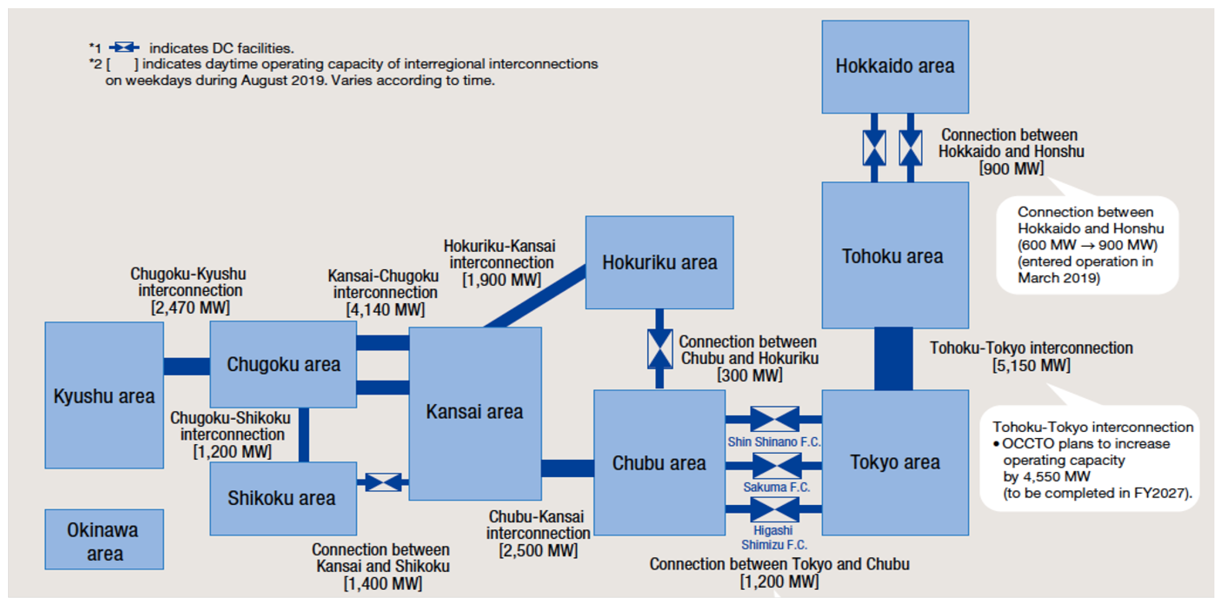
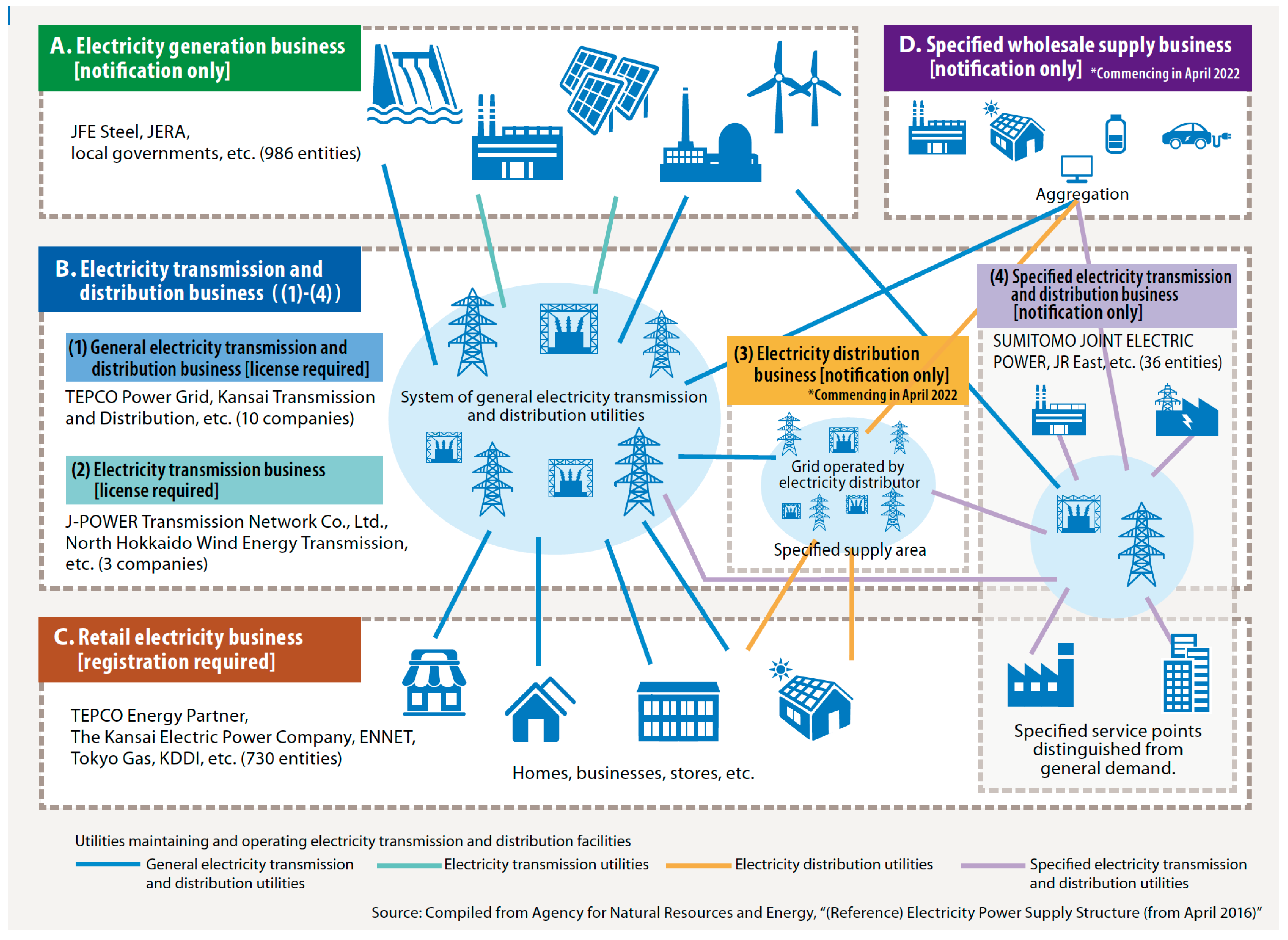
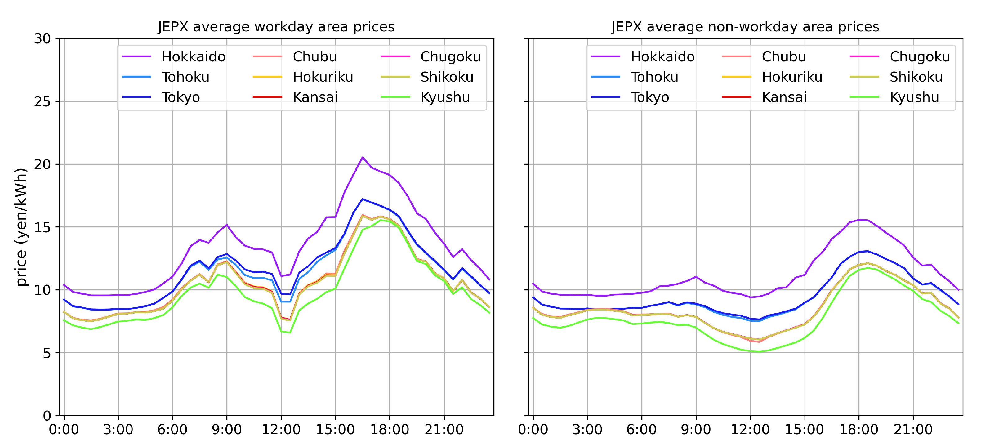
2. The Japanese Electricity Market
2.1. Introduction to the Spot Market and the Power Grid
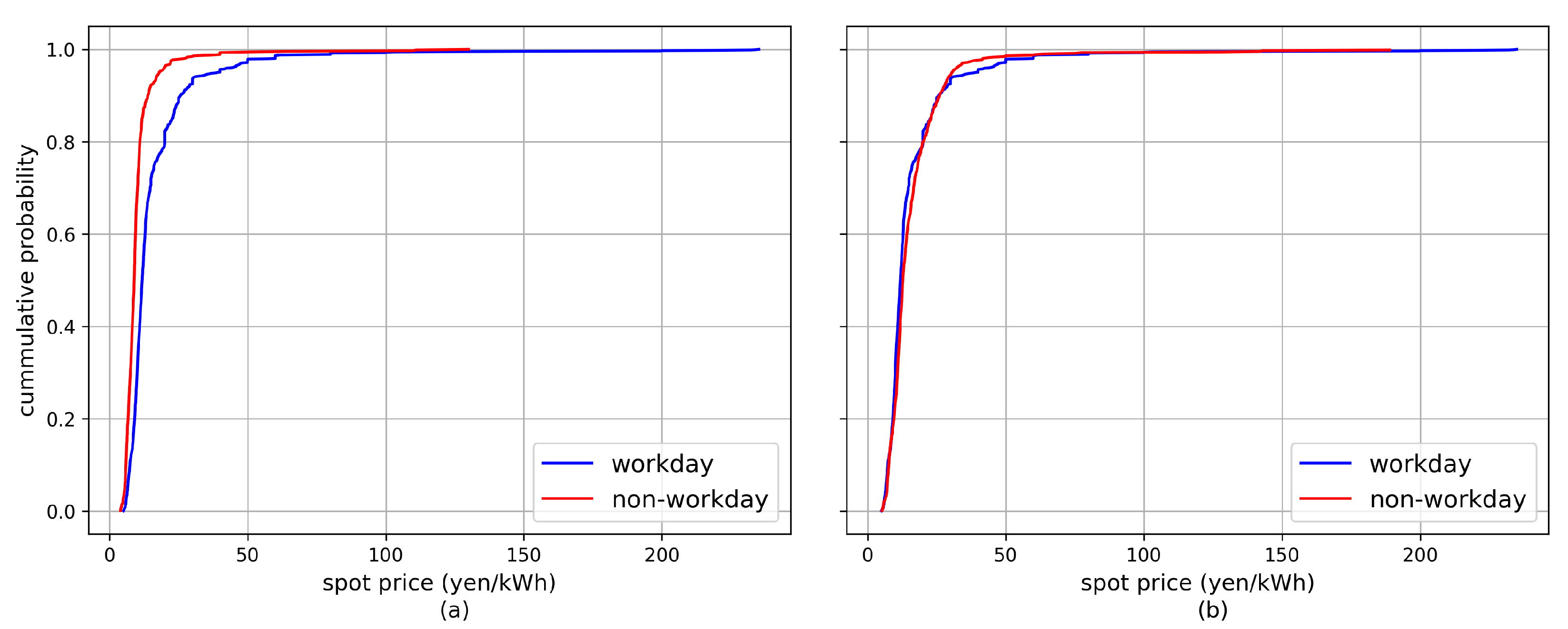
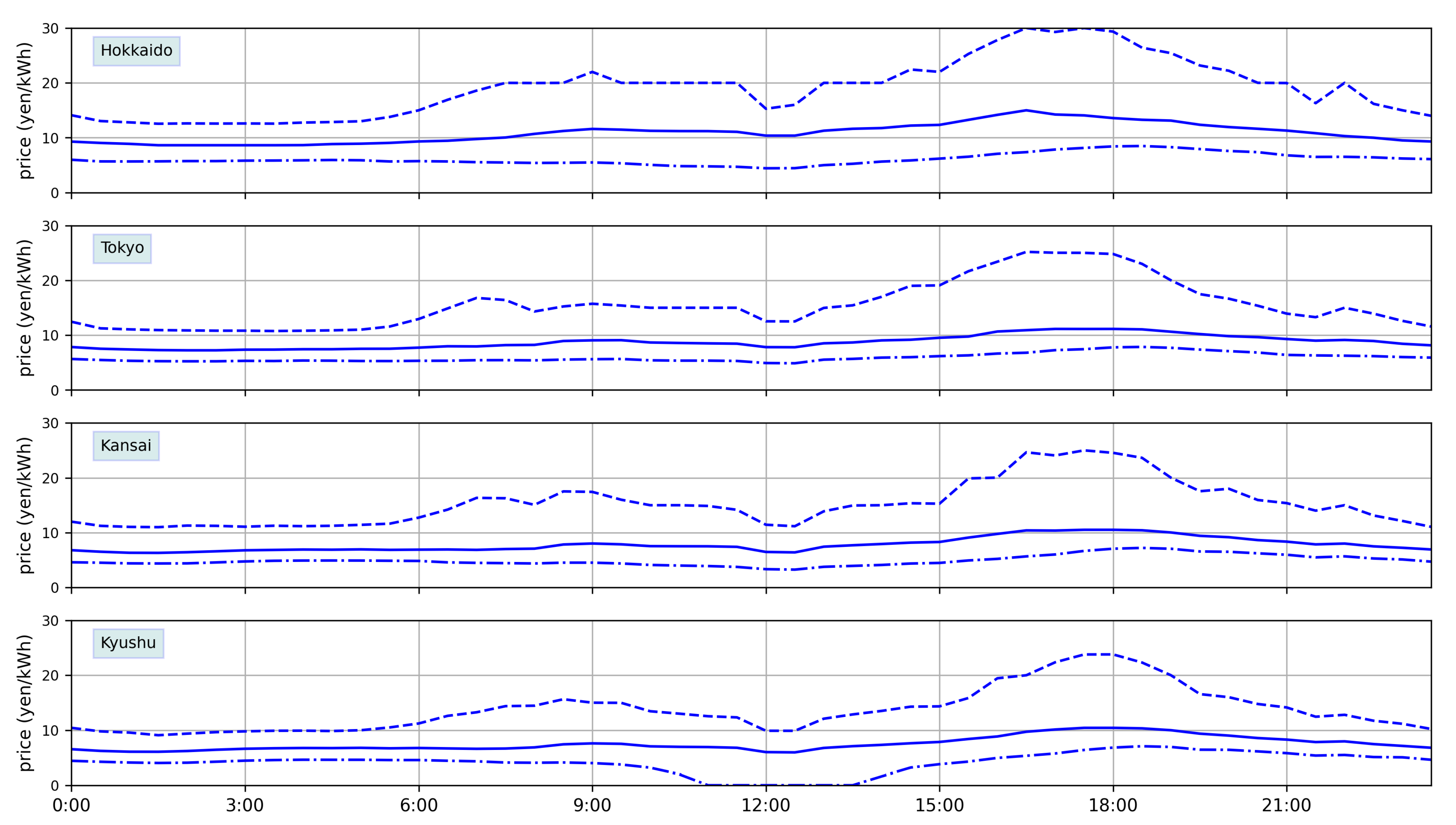
2.2. JEPX Dataset
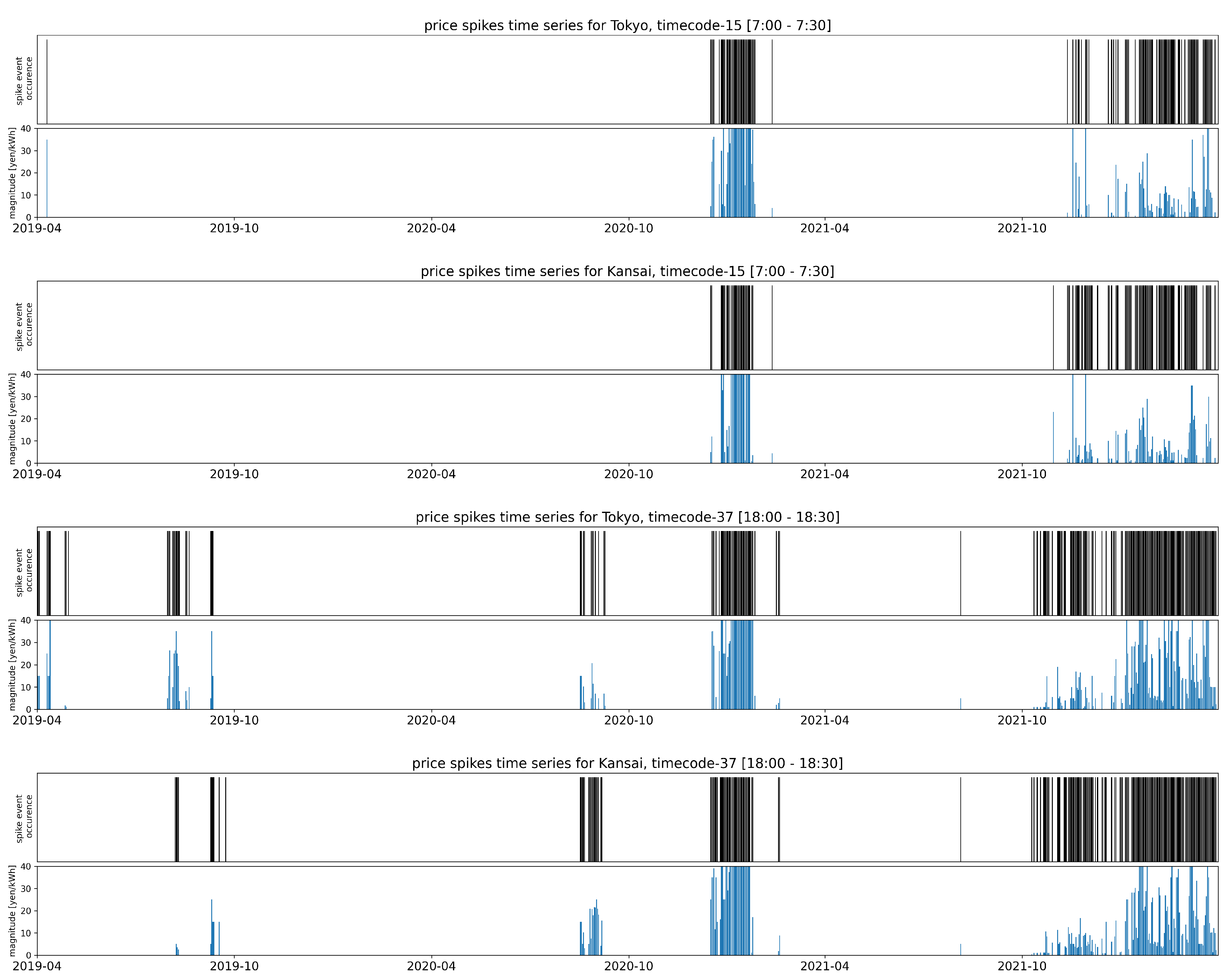
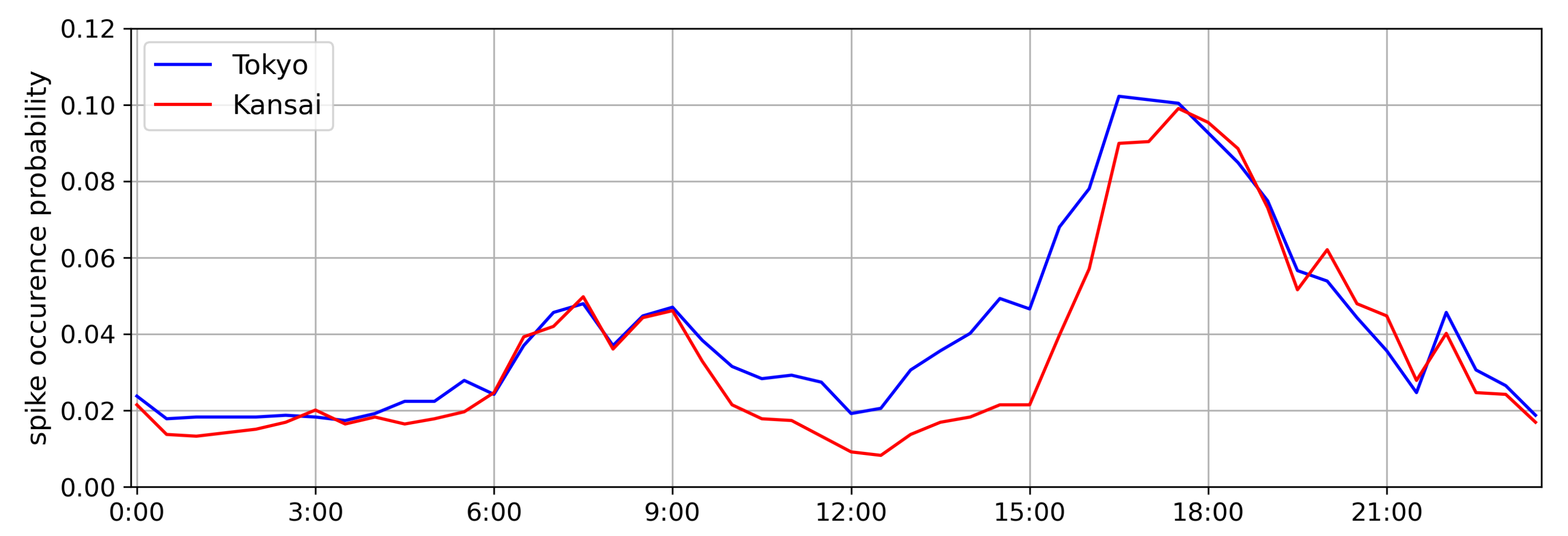
2.3. Definition of Price Spikes
3. Methodology
3.1. Notation
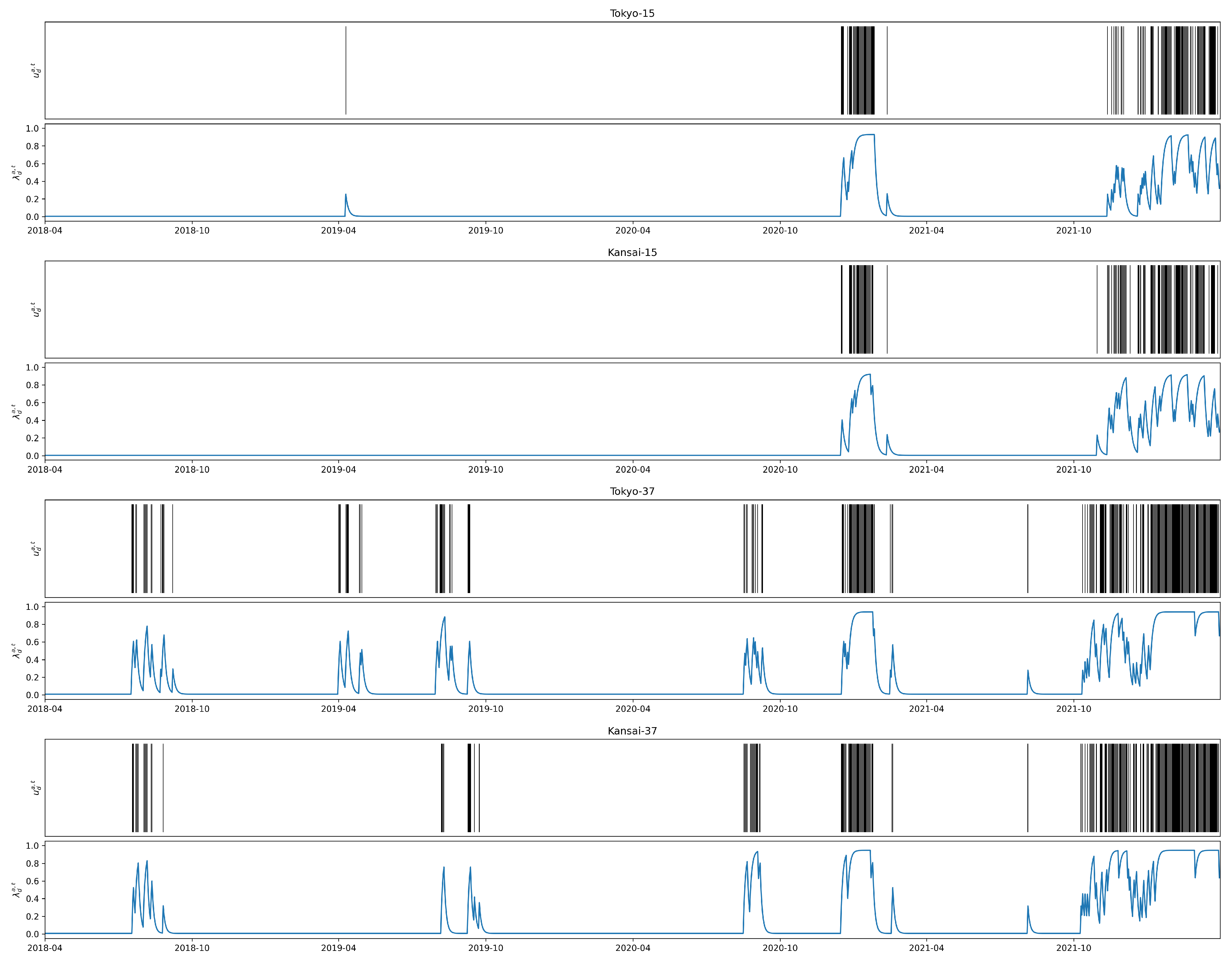
3.2. Hawkes Model
3.3. Modified Hawkes Model
3.4. Parameter Extraction
3.5. Short-Term Forecasting
4. Results
4.1. Data
4.2. Baseline Model—Persistence Model
4.3. Model Performance: Goodness of Fit
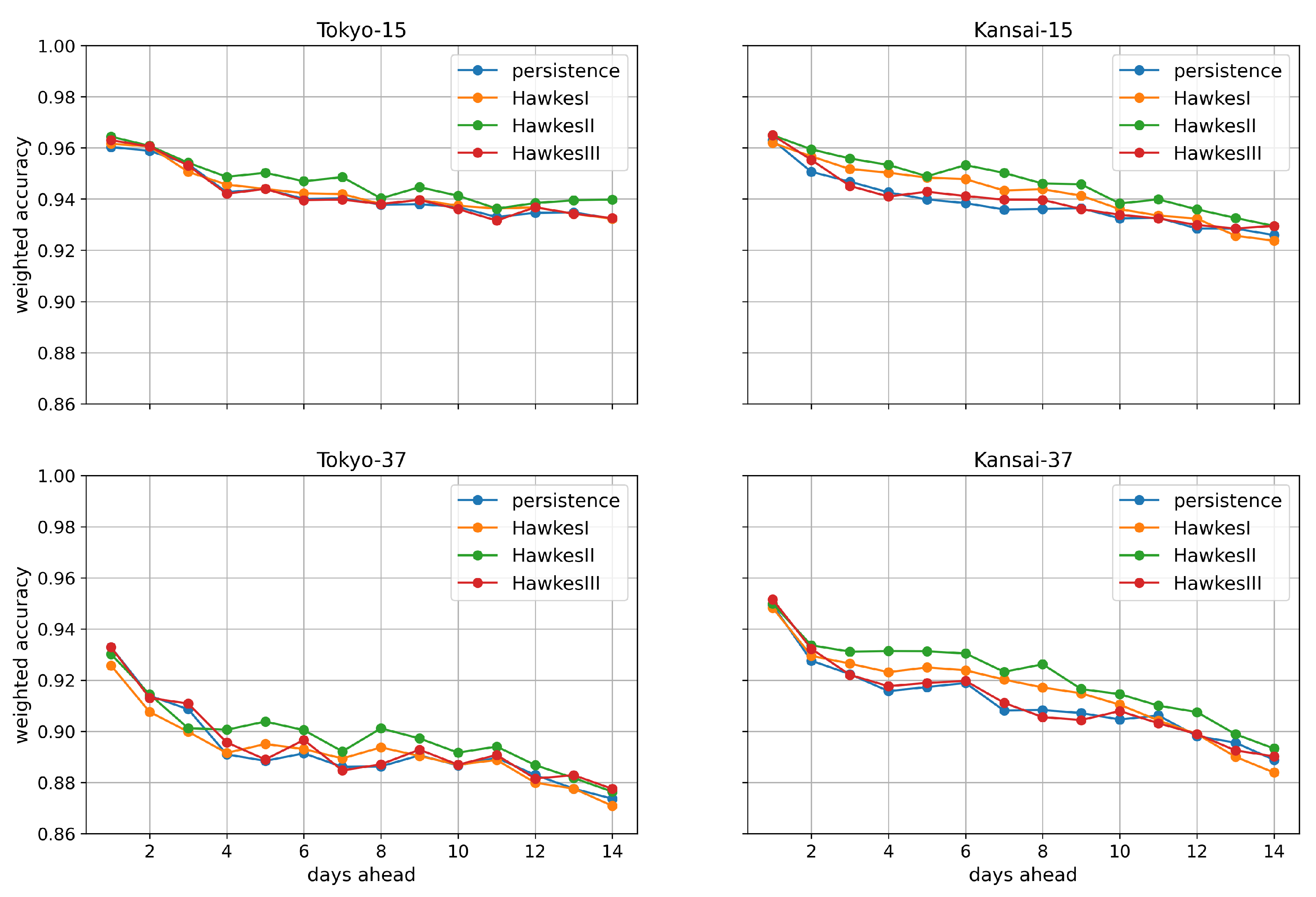
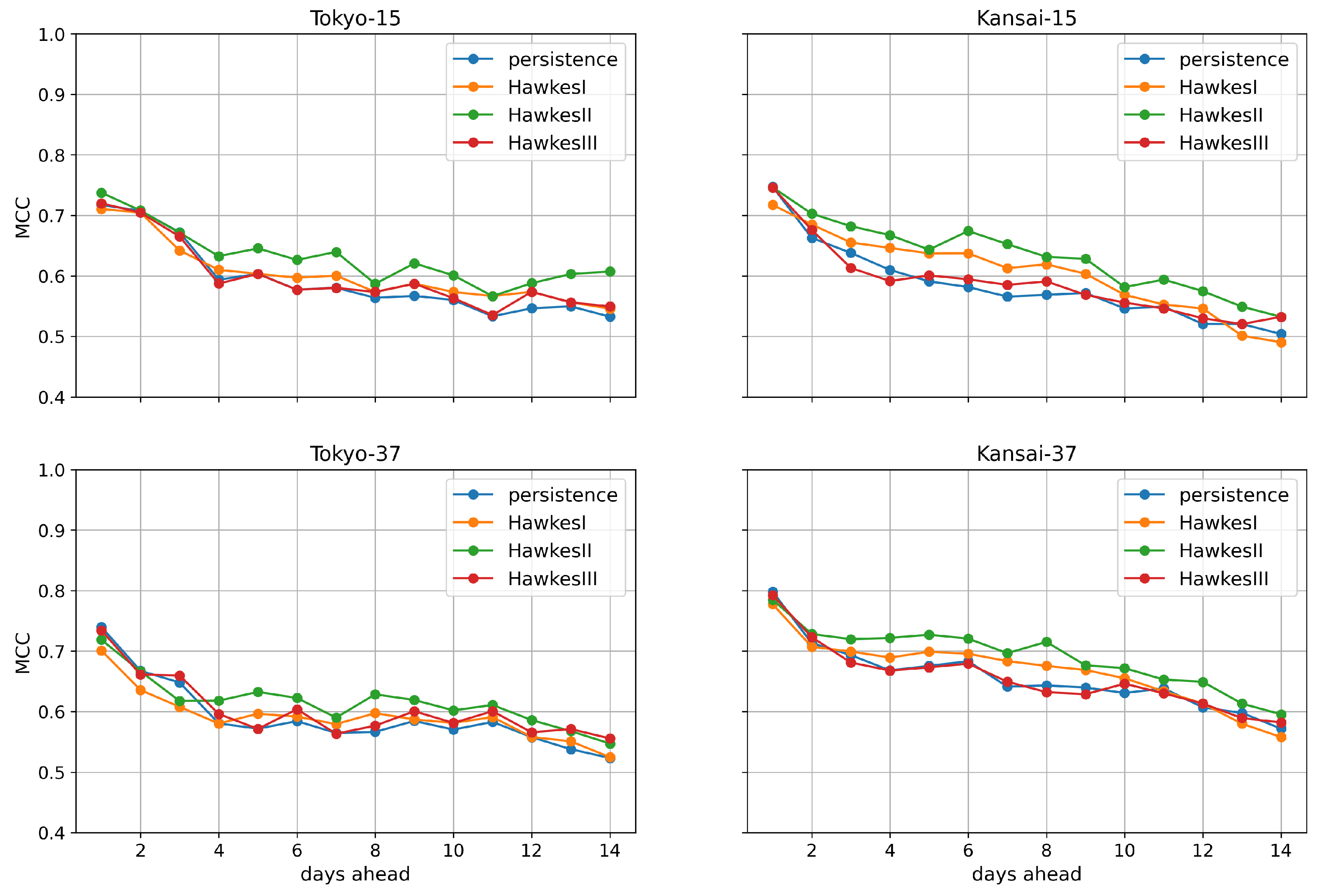
4.4. Model Performance: Spike Event Occurrence Forecasting
5. Conclusions
Author Contributions
Funding
Data Availability Statement
Conflicts of Interest
References
- Bhattacharya, K.; Bollen, M.H.; Daalder, J.E. Operation of Restructured Power Systems; Springer Science & Business Media: New York, NY, USA, 2012. [Google Scholar]
- Joskow, P.L. Lessons Learned From Electricity Market Liberalization. Energy J. 2008, 29, 9–42. [Google Scholar] [CrossRef]
- Moran, A.; Sood, R. Evolution of Global Electricity Markets; Academic Press: Waltham, MA, USA, 2013. [Google Scholar]
- Hohki, K. Outline of Japan Electric Power Exchange (JEPX). IEEJ Trans. Power Energy 2005, 125, 922–925. [Google Scholar] [CrossRef]
- Harris, C. Electricity Markets: Pricing, Structures and Economics; Wiley: West Sussex, UK, 2008. [Google Scholar]
- Shahidehpour, M.; Yamin, H.; Li, Z. Market Operations in Electric Power Systems: Forecasting, Scheduling, and Risk Management; Institute of Electrical and Electronics Engineers: New York, NY, USA; Wiley-Interscience: New York, NY, USA, 2002. [Google Scholar]
- Tsitsiklis, J.N.; Xu, Y. Pricing of fluctuations in electricity markets. In Proceedings of the 2012 IEEE 51st IEEE Conference on Decision and Control (CDC), Maui, HI, USA, 10–13 December 2012; pp. 457–464. [Google Scholar] [CrossRef]
- Gligorić, Z.; Savić, S.Š.; Grujić, A.; Negovanović, M.; Musić, O. Short-Term Electricity Price Forecasting Model Using Interval-Valued Autoregressive Process. Energies 2018, 11, 1911. [Google Scholar] [CrossRef]
- Tselika, K. The impact of variable renewables on the distribution of hourly electricity prices and their variability: A panel approach. Energy Econ. 2022, 113, 106194. [Google Scholar] [CrossRef]
- Johnathon, C.; Agalgaonkar, A.P.; Kennedy, J.; Planiden, C. Analyzing Electricity Markets with Increasing Penetration of Large-Scale Renewable Power Generation. Energies 2021, 14, 7618. [Google Scholar] [CrossRef]
- Benth, F.E.; Benth, J.S.; Koekebakker, S. Stochastic Modelling of Electricity and Related Markets; World Scientific: Singapore, 2008; Volume 11. [Google Scholar]
- Conejo, A.J.; Carrión, M.; Morales, J.M. Decision Making under Uncertainty in Electricity Markets; Springer Science+ Business Media, LLC: New York, NY, USA, 2010. [Google Scholar]
- Zedda, S.; Masala, G. Price Spikes in the Electricity Markets: How and Why. Available online: https://www.haee.gr/media/3970/s-zedda-g-masala-price-spikes-in-the-electricity-markets-how-and-why.pdf (accessed on 1 December 2022).
- Gayretli, G.; Yucekaya, A.; Bilge, A.H. An analysis of price spikes and deviations in the deregulated Turkish power market. Energy Strategy Rev. 2019, 26, 100376. [Google Scholar] [CrossRef]
- Weron, R. Electricity price forecasting: A review of the state-of-the-art with a look into the future. Int. J. Forecast. 2014, 30, 1030–1081. [Google Scholar] [CrossRef]
- Jiang, L.; Hu, G. A Review on Short-Term Electricity Price Forecasting Techniques for Energy Markets. In Proceedings of the 2018 15th International Conference on Control, Automation, Robotics and Vision (ICARCV), Singapore, 18–21 November 2018; pp. 937–944. [Google Scholar] [CrossRef]
- Nowotarski, J.; Weron, R. Recent advances in electricity price forecasting: A review of probabilistic forecasting. Renew. Sustain. Energy Rev. 2018, 81, 1548–1568. [Google Scholar] [CrossRef]
- Contreras, J.; Espinola, R.; Nogales, F.; Conejo, A. ARIMA models to predict next-day electricity prices. IEEE Trans. Power Syst. 2003, 18, 1014–1020. [Google Scholar] [CrossRef]
- Gao, G.; Lo, K.; Fan, F. Comparison of ARIMA and ANN models used in electricity price forecasting for power market. Energy Power Eng. 2017, 9, 120–126. [Google Scholar] [CrossRef]
- McHugh, C.; Coleman, S.; Kerr, D.; McGlynn, D. Forecasting Day-ahead Electricity Prices with A SARIMAX Model. In Proceedings of the 2019 IEEE Symposium Series on Computational Intelligence (SSCI), Xiamen, China, 6–9 December 2019; pp. 1523–1529. [Google Scholar] [CrossRef]
- Cifter, A. Forecasting electricity price volatility with the Markov-switching GARCH model: Evidence from the Nordic electric power market. Electr. Power Syst. Res. 2013, 102, 61–67. [Google Scholar] [CrossRef]
- Lago, J.; De Ridder, F.; De Schutter, B. Forecasting spot electricity prices: Deep learning approaches and empirical comparison of traditional algorithms. Appl. Energy 2018, 221, 386–405. [Google Scholar] [CrossRef]
- Ugurlu, U.; Oksuz, I.; Tas, O. Electricity Price Forecasting Using Recurrent Neural Networks. Energies 2018, 11, 1255. [Google Scholar] [CrossRef]
- Pórtoles, J.; González, C.; Moguerza, J.M. Electricity Price Forecasting with Dynamic Trees: A Benchmark Against the Random Forest Approach. Energies 2018, 11, 1588. [Google Scholar] [CrossRef]
- Keles, D.; Scelle, J.; Paraschiv, F.; Fichtner, W. Extended forecast methods for day-ahead electricity spot prices applying artificial neural networks. Appl. Energy 2016, 162, 218–230. [Google Scholar] [CrossRef]
- Chaâbane, N. A novel auto-regressive fractionally integrated moving average–least-squares support vector machine model for electricity spot prices prediction. J. Appl. Stat. 2014, 41, 635–651. [Google Scholar] [CrossRef]
- Li, W.; Becker, D.M. Day-ahead electricity price prediction applying hybrid models of LSTM-based deep learning methods and feature selection algorithms under consideration of market coupling. Energy 2021, 237, 121543. [Google Scholar] [CrossRef]
- Wang, J.; Yang, W.; Du, P.; Niu, T. Outlier-robust hybrid electricity price forecasting model for electricity market management. J. Clean. Prod. 2020, 249, 119318. [Google Scholar] [CrossRef]
- Mount, T.D.; Ning, Y.; Cai, X. Predicting price spikes in electricity markets using a regime-switching model with time-varying parameters. Energy Econ. 2006, 28, 62–80. [Google Scholar] [CrossRef]
- Christensen, T.; Hurn, A.; Lindsay, K. It Never Rains but it Pours: Modeling the Persistence of Spikes in Electricity Prices. Energy J. 2008, 30, 25–48. [Google Scholar] [CrossRef]
- Christensen, T.; Hurn, A.; Lindsay, K. Forecasting spikes in electricity prices. Int. J. Forecast. 2012, 28, 400–411. [Google Scholar] [CrossRef]
- Sirin, S.M.; Erten, I. Price spikes, temporary price caps, and welfare effects of regulatory interventions on wholesale electricity markets. Energy Policy 2022, 163, 112816. [Google Scholar] [CrossRef]
- HAWKES, A.G. Spectra of some self-exciting and mutually exciting point processes. Biometrika 1971, 58, 83–90. [Google Scholar] [CrossRef]
- The Electric Power Industry in Japan 2020. Available online: https://www.jepic.or.jp/pub/pdf/epijJepic2020.pdf (accessed on 8 August 2022).
- Monitoring Analytics, LLC. State of the Market Report for PJM; Monitoring Analytics: Norristown, PA, USA, 2015. [Google Scholar]
- Flatabo, N.; Doorman, G.; Grande, O.; Randen, H.; Wangensteen, I. Experience with the Nord Pool design and implementation. IEEE Trans. Power Syst. 2003, 18, 541–547. [Google Scholar] [CrossRef]
- Bradbury, K.; Pratson, L.; Patiño-Echeverri, D. Economic viability of energy storage systems based on price arbitrage potential in real-time U.S. electricity markets. Appl. Energy 2014, 114, 512–519. [Google Scholar] [CrossRef]
- Ott, A. Experience with PJM market operation, system design, and implementation. IEEE Trans. Power Syst. 2003, 18, 528–534. [Google Scholar] [CrossRef]
- The Electric Power Industry in Japan 2022. Available online: https://www.jepic.or.jp/pub/pdf/epijJepic2022.pdf (accessed on 8 August 2022).
- The Japan Electric Power Exchange Website. Available online: http://www.jepx.org/english/index.html (accessed on 8 August 2022).
- Hawkes, A.G.; Oakes, D. A cluster process representation of a self-exciting process. J. Appl. Probab. 1974, 11, 493–503. [Google Scholar] [CrossRef]
- Embrechts, P.; Liniger, T.; Lin, L. Multivariate Hawkes processes: An application to financial data. J. Appl. Probab. 2011, 48, 367–378. [Google Scholar] [CrossRef]
- Chicco, D.; Jurman, G. The advantages of the Matthews correlation coefficient (MCC) over F1 score and accuracy in binary classification evaluation. BMC Genom. 2020, 21, 6. [Google Scholar] [CrossRef]
- Boughorbel, S.; Jarray, F.; El-Anbari, M. Optimal classifier for imbalanced data using Matthews Correlation Coefficient metric. PLoS ONE 2017, 12, e0177678. [Google Scholar] [CrossRef]


| Area | Mean | Median | Std. Dev | Skewness | 95th Percentile |
|---|---|---|---|---|---|
| Hokkaido | 12.72 | 10.54 | 12.01 | 8.90 | 25.67 |
| Tohoku | 10.82 | 8.67 | 11.75 | 9.83 | 23.00 |
| Tokyo | 10.93 | 8.71 | 11.85 | 9.67 | 23.37 |
| Chubu | 9.91 | 7.66 | 10.96 | 9.48 | 21.87 |
| Hokuriku | 9.89 | 7.66 | 10.94 | 9.53 | 21.54 |
| Kansai | 9.88 | 7.66 | 10.93 | 9.57 | 21.24 |
| Chugoku | 9.87 | 7.65 | 10.93 | 9.57 | 21.24 |
| Shikoku | 9.86 | 7.65 | 10.95 | 9.61 | 21.22 |
| Kyushu | 9.16 | 7.36 | 10.69 | 10.21 | 19.45 |
| log L | Tokyo-15 | Kansai-15 | Tokyo-37 | Kansai-37 |
|---|---|---|---|---|
| Persistence | − 207.7 | −204.5 | −333.9 | −271.3 |
| Hawkes I | −141.9 | −147.8 | −256.4 | −209.9 |
| Hawkes II | −133.0 | −135.4 | −248.2 | −199.6 |
| Hawkes III | −200.9 | −198.6 | −317.1 | −263.4 |
| MAE | Tokyo-15 | Kansai-15 | Tokyo-37 | Kansai-37 |
|---|---|---|---|---|
| Persistence | 0.0730 | 0.0738 | 0.1331 | 0.1112 |
| Hawkes I | 0.0733 | 0.0771 | 0.1343 | 0.1168 |
| Hawkes II | 0.0676 | 0.0702 | 0.1251 | 0.1045 |
| Hawkes III | 0.0741 | 0.0806 | 0.1301 | 0.1201 |
| WACC | Tokyo-15 | Kansai-15 | Tokyo-37 | Kansai-37 |
|---|---|---|---|---|
| Persistence | 0.9419 | 0.9384 | 0.8929 | 0.9120 |
| Hawkes I | 0.9441 | 0.9435 | 0.8923 | 0.9164 |
| Hawkes II | 0.9466 | 0.9468 | 0.8980 | 0.9211 |
| Hawkes III | 0.9422 | 0.9401 | 0.8947 | 0.9128 |
| MCC | Tokyo-15 | Kansai-15 | Tokyo-37 | Kansai-37 |
|---|---|---|---|---|
| Persistence | 0.5937 | 0.5845 | 0.5917 | 0.6576 |
| Hawkes I | 0.6043 | 0.6065 | 0.592 | 0.6676 |
| Hawkes II | 0.6317 | 0.6339 | 0.6167 | 0.6915 |
| Hawkes III | 0.5995 | 0.5903 | 0.6034 | 0.6569 |
Disclaimer/Publisher’s Note: The statements, opinions and data contained in all publications are solely those of the individual author(s) and contributor(s) and not of MDPI and/or the editor(s). MDPI and/or the editor(s) disclaim responsibility for any injury to people or property resulting from any ideas, methods, instructions or products referred to in the content. |
© 2023 by the authors. Licensee MDPI, Basel, Switzerland. This article is an open access article distributed under the terms and conditions of the Creative Commons Attribution (CC BY) license (https://creativecommons.org/licenses/by/4.0/).
Share and Cite
Adline, B.; Ikeda, K. A Hawkes Model Approach to Modeling Price Spikes in the Japanese Electricity Market. Energies 2023, 16, 1570. https://doi.org/10.3390/en16041570
Adline B, Ikeda K. A Hawkes Model Approach to Modeling Price Spikes in the Japanese Electricity Market. Energies. 2023; 16(4):1570. https://doi.org/10.3390/en16041570
Chicago/Turabian StyleAdline, Bikeri, and Kazushi Ikeda. 2023. "A Hawkes Model Approach to Modeling Price Spikes in the Japanese Electricity Market" Energies 16, no. 4: 1570. https://doi.org/10.3390/en16041570
APA StyleAdline, B., & Ikeda, K. (2023). A Hawkes Model Approach to Modeling Price Spikes in the Japanese Electricity Market. Energies, 16(4), 1570. https://doi.org/10.3390/en16041570