Abstract
In recent years, the integration of battery energy storage systems (BESSs) with multilevel modular converters (MMCs) has received interest in power system applications. In this work, this configuration is called a MMC-based BESS. The batteries are connected directly to the MMCs on submodules (SMs), called the single-stage approach. Several control strategies have been proposed to guarantee the proper operation of a MMC-based BESS. This system is complex due to the control strategy. Another challenge is in obtaining the controller gains for a MMC-based BESS converter. In this sense, there is a gap in the methodology used to calculate the controller gains. Thus, this work aimed to tune the analytical expressions of a MMC-based BESS by considering the single-stage approach. The methodology is validated through detailed simulation models of 10.9 MVA/5.76 MWh connected to a 13.8 kV power system. Finally, to validate the dynamics of the controllers, the simulation results in the PLECS software for the charging and discharging processes are presented.
1. Introduction
Renewable energy sources (RESs), such as photovoltaic (PV) and wind power plants (WPPs) are presented as solutions that support the modern energy system. However, uncertainty and intermittency in generation can cause power fluctuations [1,2]. As a consequence, the stability of the electrical system can be affected. Battery energy storage systems (BESSs) are used as alternatives to increase the penetration of RESs into the power system [3].
BESSs are beneficial, i.e., due to their flexibility in installation locations, shorter construction times (regarding facilities), and quick response times to system events. BESSs are gaining more space in the electric power market due to the numerous applications in systems related to generation, transmission, and distribution. In recent years, there has been an increase in BESS facilities worldwide, totaling over 17 GW at the end of 2020 [4]. Different battery technologies can be used in the grid, such as NiMH, NiCd, Pb-acid, and Li-ion [5]. According to [2], currently, Li-ion batteries are the most used in low-, medium-, and high-powered applications.
The connection between a BESS and the grid is carried out through power electronics. The battery bank can be directly connected to the grid by a DC/AC converter or decoupled by a DC/DC stage [6]. Different topologies can be used to implement BESSs, including two-level voltage–source converters (VSCs) and multilevel converters [2,7]. Among them, the multilevel modular converter (MMC) is a promising alternative due to its characteristics, such as reliability, scalability, high efficiency, effective redundancy, and functionality [8,9,10]. Furthermore, a MMC is able to provide high-output voltage using low-voltage switches. In addition, a low number of batteries in series is required [11]. The integration of BESS with the MMC is called MMC-based BESS.
Figure 1 presents the MMC-based BESS topology studied in this paper. The MMC is characterized by the bidirectional submodule (SM) cascade connected on each converter arm [12]. The SM is a half-bridge converter composed of two insulated-gate bipolar transistors (IGBTs) and two diodes. In a MMC-based BESS system, the battery arrangement can be connected directly to the DC-link (called centralized) or connected directly to each SM of the converter (called distributed) [13]. In this paper, the distributed configuration is adopted. In addition, in this configuration, the batteries can be connected directly to the SM (single-stage) or interfaced by a DC/DC converter (two-stage) [10,14].
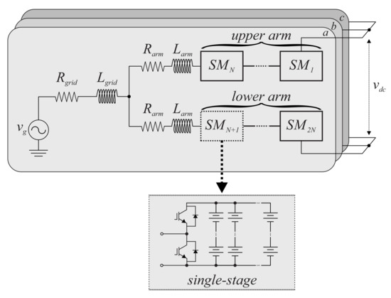
Figure 1.
Schematic of a MMC topology.
In systems that use MMC-based BESSs, the SM half-bridge configuration implies low-frequency currents at the outputs. In the single-stage approach, as the battery rack connection is direct to the SM, the current flowing to the battery has low-order harmonic content [2]. These components are mainly first- and second-order. As a consequence, the root-mean-square (RMS) value of the current, the temperature, and the internal losses in the battery increase. These variations may decrease the battery’s lifetime [6,15,16].
Another challenge with the MMC-based BESS is the control strategy. In this type of system, the control used needs to evaluate the energy flow. When using batteries, an imbalance with the state-of-charge (SOC) can occur due to some hypotheses, such as different technologies, different battery lifetimes, or failure in a SM. Therefore, a SOC balancing algorithm must be implemented [17,18]. Finally, in systems with unbalanced grids, it needs a control capable of evaluating each MMC phase independently.
References [17,19] present the control strategies that apply to the single-stage approach. In [3,20,21], control methods for the two-stage approach are discussed. However, in these works, control tuning is not presented. This poses challenges for researchers who intend to investigate or compare such control schemes. Conversely, MMC is a converter topology with a relatively complex structure with several control objectives. In order to fill this gap, this work proposes a tuning methodology based on analytical expressions for MMC-based BESS controllers. The objective is to provide a straightforward way to compute the controller gain, which is very useful for those who want to investigate challenges in a MMC-based BESS that are not directly coupled to the control scheme, but require a proper control operation (e.g., modulation scheme, efficiency, redundancy, fault tolerance, etc.).
This paper is outlined as follows: Section 2 presents the mathematical model of the MMC. Then, the main circuit parameters design for a single-stage approach is presented. In Section 3, the control strategy for the MMC-based BESS is presented. Section 4 presents the case study for a single-stage approach. In order to validate the presented methodology, all controllers are analyzed with respect to frequency and step response. In Section 5, the methodology for control-tuning is presented. Section 6 presents the simulation results, considering the charging and discharging processes of the batteries for the single-stage approach. Finally, the conclusions are stated in Section 7.
2. Mathematical Models
2.1. MMC
The mathematical model presented in this section defines the main variables that describe the MMC dynamics. In addition, the instantaneous power flow in MMC is modeled, which leads to some conclusions regarding the capacitor voltage balancing and voltage ripple. Voltage sources represent the voltages generated by each arm. denotes the voltage synthesized in the upper arm of phase-n while denotes the voltage synthesized in the lower arm of phase-n. The following assumptions are adopted:
- 1.
- The effect of the switching frequency is neglected, i.e., an average model is considered;
- 2.
- The capacitor voltages are assumed to be perfectly balanced.
Under such conditions, the converter presented in Figure 1 can be represented by Figure 2. This model assumes perfect balancing capacitor voltages and negligible harmonic components.
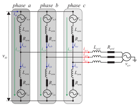
Figure 2.
MMC arm-average model for and dynamics evaluation.
In the distributed topology, the DC-link current () is zero. In this way, the sum of the upper and lower arm currents must be zero. Accordingly,
where is the upper arm current of phase-n and is the lower arm current of phase-n.
According to [22], the arm currents can be written as follows:
where is grid current of phase-n and is the circulating current of phase-n. The can be indirectly measured through the arm currents as follows:
The superposition theorem can be employed to analyze the output current and the circulating current independently. The output current dynamics are described by the per-phase circuit shown in Figure 3.
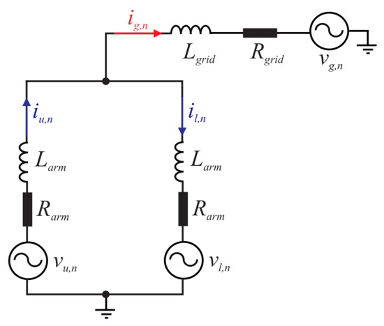
Figure 3.
Equivalent circuit of the output current dynamics.
The analysis of Figure 3 leads to:
where is the line-to-neutral output voltage, which can be expressed by:
It is important to remark that the factor in Equations (5) and (6) are due to Millman’s theorem. Reference [23] any association with the connected voltage sources in parallel can be reduced to just one equivalent source. The same conclusion can be obtained through Thevenin’s theorem.
The dynamics can be obtained as follows:
where is the internal voltage. The normalized reference signals per n-phase are given by:
where is the output reference of the individual voltage balancing control. However, is disregarded as close to zero.
The insertion index for the upper and lower arms, respectively, are given by:
where is the SM voltage reference and N is the total number of SMs.
At this point, two facts must be highlighted. First, the control of the output current guarantees the power exchange between the batteries and the electrical grid. On the other hand, the circulating current control plays an important role in the energy balance among the converter arms. The expressions of instantaneous power developed by each arm in a steady state are derived to explicitly show these facts. The instantaneous active power in the lower arm of phase-n () and the instantaneous active power in the upper arm of phase-n () of the system can be estimated by:
Equation (11) can then be rewritten as follows:
Assuming the contribution of the internal voltage of phase-n, () small, Equation (12) can be simplified. Accordingly:
Different colors are employed in relation to Equation (11) to highlight the power terms with different physical meanings. At this point, the following conclusions can be stated:
- 1.
- The product leads to a DC component and the second-harmonic power oscillation. Assuming that and are sinusoidal waves, the average value represents the active power transferred from the submodules to the grid. The oscillating component leads to a second-harmonic ripple in the battery current.
- 2.
- Product leads to a fundamental frequency oscillating power. This term results in a fundamental frequency ripple in the battery current. As observed, this term presents opposite signals in the lower and upper arms. Therefore, this power oscillation is not observed at the converter AC terminals.
- 3.
- The parcels containing require more attention. As previously mentioned, a possible solution for Equation (4) is given by:with free and . The term indicates that a DC component in a circulating current component can perform the energy exchange between the converter phases. Indeed, the sum of the power transfer for the three phases must be zero, which becomes evident in the energy exchange among the converter phases.
- 4.
- The term indicates that a fundamental frequency–circulating current leads to a non-zero power in the arm. Moreover, these terms present opposite signals in the upper and lower arms. Therefore, a fundamental frequency–circulating current can exchange energy between the lower and upper arms.
2.2. Battery
Figure 4 presents the detailed model of the battery. Two models are used in this system: electric and thermal. In the electrical model, the current source receives updated values at all times obtained from the division between the power of a SM and the OCV of the battery. Through the battery current and other parameters with , , , and the battery mission profile, it is possible to obtain the SOC over time. Finally, the impedance of the battery at this moment is represented by .
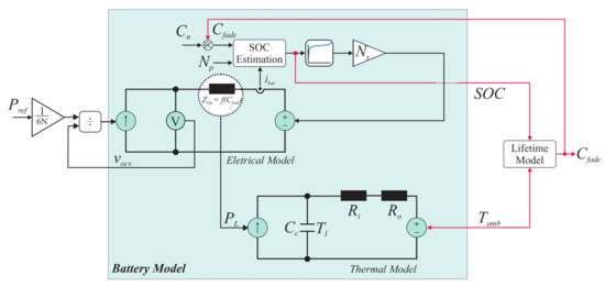
Figure 4.
Structure of the battery model.
With the electrical model of the battery, the next step is to represent the thermal model. This equivalent model presents some simplifications so that several experimental measurements are not necessary. The battery surface temperature is assumed to be uniform. In this sense, three parameters are considered: internal heat transfer resistor (), external heat transfer resistor (), and heat capacity (). These parameters were estimated from experimental data [24]. is the power of each battery and is the ambient temperature in Kelvin. Finally, the internal temperature of the battery () can be analyzed during the battery operation. In addition, the battery temperature is used in the lifetime estimation procedure. The procedure for calculating the battery lifetime is presented in [10].
3. MMC-Based BESS Control Strategy
The control strategy used in a MMC-based BESS can be divided as follows:
- Grid current control;
- SOC-balancing control;
- Circulating current control.
Figure 5 shows the complete control strategy of a MMC-based BESS.
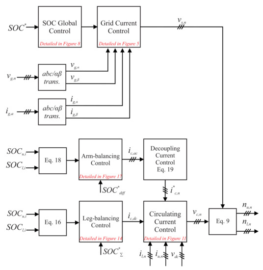
Figure 5.
Overview of the MMC-based BESS control strategy.
The grid current control is implemented in the stationary reference frame () coordinates [22]. Proportional resonant (PR) controllers are used to control the active power exchange with the grid.
The active power reference in the grid current control depends on the operating status of the MMC topology. In the process of battery charging or discharging, the reference is derived from the global SOC control. Therefore, is obtained based on the proportional–integral (PI) controller. On the other hand, in the case of an external power reference, the current reference is computed by:
where is the peak of the line-to-neutral voltage.
The leg-balancing control guarantees that all converter phases present the same average SOC. The average SOC of each phase n is computed by the:
where is the SOC of the i- SM battery rack in the upper arm of phase n and is the SOC of the i- SM battery rack in the lower arm of phase n. The SOC reference in leg-balancing control is computed by the average SOC in the converter phases:
The leg-balancing controller computes the DC circulating current component responsible for the exchange of energy in the converter phases. Therefore, it ensures that all legs have the same average SOC.
For the arm-balancing control, the average SOC balancing in the upper and the lower arms is performed. The SOC difference in each converter phase, (), is computed through the proportional controller. The is expressed as follows:
In the arm-balancing control, the is set to zero to guarantee SOC balancing in the arms of each phase. This controller computes the fundamental frequency circulating current responsible for the energy exchange in the upper and lower arms. Since the leg-balancing control (or horizontal balancing) and arm-balancing control (or vertical balancing) compute different components of the circulating current, these controllers can have similar bandwidths. The arm energy control can be designed with a bandwidth similar to the leg energy control [25].
However, the circulating current of one phase must be the linear combination of the other two. Therefore, this work uses the decoupling network discussed in [26]. This proposal injects an active current in the unbalanced phase and a reactive current in the balanced phase. Thus, the averages of the SOC are not displaced and the difference in the average energy is not affected. For example, if phase A has an SOC error (), the SOC error in phases B and C are zero ( and ); a fundamental frequency component in the phase with the grid voltage must circulate in phase A to guarantee the active power exchange. On the other hand, the fundamental frequency circulating currents are selected to be 90 degrees (lead or lag) to the grid voltage in phases B and C, leading to the (now active) power exchange. It is important to remark that the sum of the circulating currents will be zero if the amplitude of the circulating currents is properly computed. In this way, the circulating current references computed by the arm balancing control are given by:
where is the proportional gain of the arm balancing control and is the fundamental angular frequency obtained by PLL.
It is important to remark that the global SOC control and the leg-balancing control do not operate at the same time. When the MMC-based BESS operates in the charging/discharging mode, the global SOC control computes the current reference of each phase, which leads to a balance of the average SOC of the three phases. Under such conditions, the leg-balancing control is disabled. However, when the MMC-based BESS provides ancillary services, the global SOC-balancing control is disabled. Under such conditions, the leg-balancing control is enabled and the leg-balancing control is obtained based on a DC circulating current.
The insertion index calculated in Equation (9) is applied in the modulation strategy. Regarding the modulation strategy, the PS-PWM is employed. The injection of one-sixth of the third harmonic is considered to extend the linear region of the modulator.
4. Case Study
The case study employed in this work is based on Ref. [6]. This reference presents a methodology to perform the sizing of the MMC-based BESS. The case study is based on a 10.9 MVA/5.76 MWh system connected to a 13.8 kV power system, which provides ancillary services for a PV power plant. The MMC-based BESS in this study is composed of Li-ion cells. The input parameters of the MMC-based BESS studied in this paper are presented in Table 1.

Table 1.
Parameters of the MMC-based BESS.
The battery cell ANR26650M1-B manufactured by A123 systems is employed [27]. The main battery cell data are presented in Table 2.
Table 2.
Parameters of the battery cell ANR26650M1-B [27].
Based on the parameters presented, the next section discusses the control strategy and the control-tuning methodology.
5. Control Tuning
In order to validate the methodology for control tuning, after each control, the analysis of the frequency and step response is performed. It is worth mentioning that all controllers were discretized by the Tustin method (trapezoidal). Moreover, the delay in digital implementation is included in the model.
Finally, the gains for all controllers were calculated neglecting the sensor gains. This inherently assumes that, in practice, the sensor presents a higher bandwidth than the control loop requirements.
5.1. Grid Current
Figure 6 shows the block diagram with the closed control loop for the grid current control. represents the proportional resonant (PR) compensator, given by:
where is the proportional gain and the resonant gain. In this control loop, the resonance frequency is the grid frequency. The effect of the implementation delay and the zero-order hold can be represented by the following transfer function, [28,29]:
where is the sampling time. Finally, the plant grid current transfer function can be represented by:
where and .
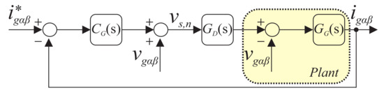
Figure 6.
Block diagram for the strategy for controlling the grid current.
The open-loop transfer function for the grid current control can be written as follows:
The control-tuning of the current loop follows the methodology discussed in [22]. The objective is to maximize the current control bandwidth. Based on this methodology, the following tuning formulas are obtained:
where is the resonant part bandwidth and is the desired closed-loop system bandwidth. Thus, there is an upper limit to for the closed-loop system to remain stable. In this work, consider , at least of the grid frequency. In order to simplify the closed-loop transfer function, consider . In this work, .
The gain is obtained considering the transfer function of Equation (22) in a closed loop with a pure proportional gain. According to [22], the bandwidth of the closed-loop system is an important parameter. It determines the exponential convergence rate for transients of the closed-loop system. The gain is the product of the angular frequency and impedance, or equivalently, angular frequency-squared times inductance.
Figure 7 shows the open-loop Bode diagram for the output grid’s current control. The control features a margin gain of 9.93 dB at 1.33 kHz and a phase margin of 57.6 at 409 Hz. Furthermore, we can see the effect of using the resonant controller in the 60 Hz range, as shown in Equation (20).
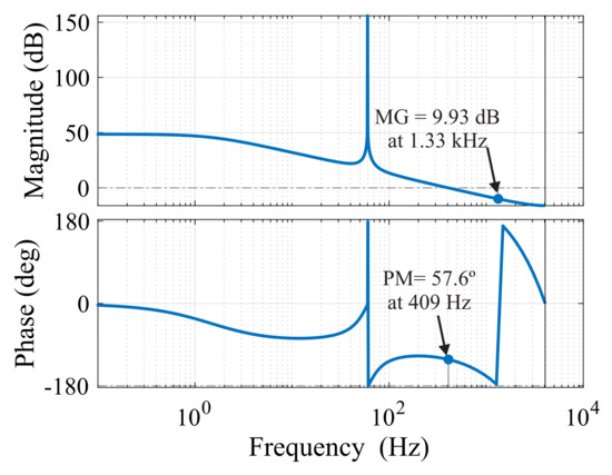
Figure 7.
Output grid current controller’s open-loop Bode diagram plot.
The performance of the output grid current controller in tracking a sinusoidal reference was evaluated in a 0.30 s simulation. According to Figure 8, up to 0.15 s, the reference is 0, after which a unit reference is given. The system takes approximately 0.02 s to reach the reference.
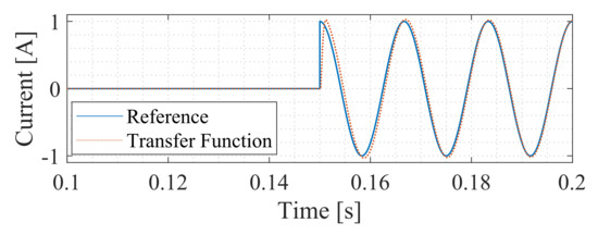
Figure 8.
Output grid current controller step response.
5.2. Global SOC Control
The plant transfer function can be obtained by neglecting the converter losses and assuming an even distribution of the energy among the converter cells. Under such conditions, the following expression can be obtained for the battery current:
where is the peak of the output voltage of the SM, is the battery voltage, is the peak of the converter output current, and are the number of series and parallel battery strings, respectively.
In addition, the battery SOC can be obtained as:
where is the battery capacity.
In this system, a PI controller is used. Then, the transfer function is given by:
The block diagram of the SOC global control is presented in Figure 9.
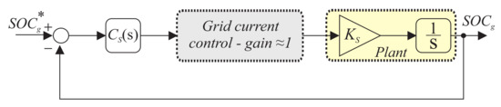
Figure 9.
Block diagram of the global SOC control.
The open-loop transfer function is given by:
The closed-loop transfer function can be written as follows:
Note that Equation (32) is equivalent to the following expression:
The tuning of the controllers is carried out by the pole placement method. This proposal defines the gains for the poles of the transfer function in a closed loop as being real, allocated in the left semi-plane, and considering the closed-loop poles as and . Moreover, we assume that and . Thus,
Thus, the following tuning formulas are obtained:
where and are the poles of the closed-loop transfer function. Typically, the poles are separated by a decade. In addition, the value of the largest must be allocated at least a decade below the cutoff frequency of the grid current. In this way, it guarantees the proper functioning of the cascade control.
According to Figure 9, in the global SOC, the control strategy used considers the internal loop of the output current and the external loop of the global SOC control. The open-loop frequency response for the global SOC control is shown in Figure 10. The control has a gain margin of 75.4 dB at 4.05 kHz and a phase margin of 85.3 at 0.441 Hz. Two Bode diagrams are presented: in the solid line, considering the ideal internal current loop (gain = 1), and in the dashed line, considering the insertion of the internal current loop. Note that for high frequencies the curves are not similar. This is due to the fact that it is above the current loop cutoff frequency.
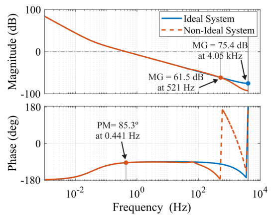
Figure 10.
Output global SOC controller–open-loop Bode plot.
Figure 11 presents the step response for the closed-loop system considering the ideal and non-ideal systems. With slower dynamics than the output grid current control, the global SOC control needs approximately 2.5 s to reach the reference.
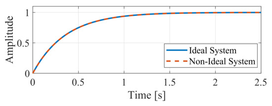
Figure 11.
Global SOC controller step response.
5.3. Circulating Current Control
The circulating current control block diagram is presented in Figure 12. In this control project, is the PR controller, represented by:
where and refer to the proportional and resonant gains of the circulating current controller.
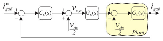
Figure 12.
Block diagram of the circulating current control.
The plant transfer function of the circulating current controller is given by:
According to Section 5.1, the gains of the PR controller can be calculated according to the following formula:
where is the resonant part of the bandwidth and is the desired closed-loop system bandwidth. Consider , at least of the grid frequency. In order to simplify the closed-loop transfer function, consider . In this work, .
The open-loop Bode diagram of the circulating current control is shown in Figure 13. The system frequency response has a stable response at 241 Hz. Furthermore, according to Equation (34), the resonant control used is allocated at 60, 120, and 240 Hz.
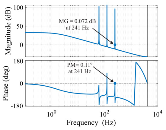
Figure 13.
Circulating current controller–open-loop Bode diagram.
The performance of the circulating current controller in tracking a sinusoidal reference is evaluated in Figure 14. The following sinusoidal reference presents the fundamental-, second-, and fourth-order harmonic components with unity amplitudes and phase 0. Note that the control tuning allows the circulating current to follow the reference as desired.
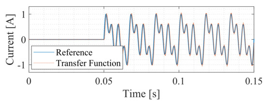
Figure 14.
Circulating current controller’s step response.
5.4. Leg-Balancing Control
In order to obtain the system transfer function, the converter losses are disregarded and uniform energy distribution is assumed between the converter cells. With this, the DC portion of the current in the battery can be calculated as follows.
In addition, the battery SOC can be obtained as:
Therefore, the following transfer function is obtained:
where is the DC component of the peak current and is given by:
In this system, a PI controller is used. Then, the transfer function, , is given by:
The block diagram of the leg-balancing control is presented in Figure 15. The open-loop transfer function is given by:
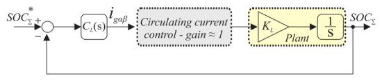
Figure 15.
Block diagram of the leg-balancing control.
Using a similar procedure in Section 5.2, the following tuning formulas are obtained:
where and are the poles of the closed-loop transfer function.
In the leg-balancing control, the external loop has the total SOC per phase as the input. The controller output sends a current reference to the internal circulating current loop. Considering that the external loop has slower dynamics than the circulating current loop, the leg-balancing control is allocated to four decades of the circulating current control. The system has a gain margin of 95.4 dB at 4.05 kHz and a phase margin of 85.3 at 0.0442 Hz. Figure 16 shows the Bode diagram for the ideal and non-ideal systems. Note that for frequencies below 122 Hz, the behaviors are the same. However, for frequencies greater than the current loop cutoff frequency, the behaviors do not follow the ideal loop.
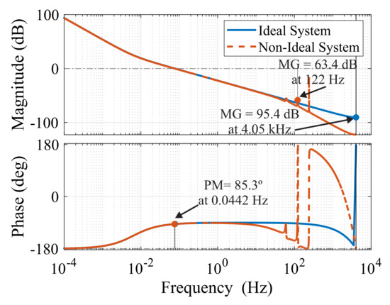
Figure 16.
Leg-balancing controller–open-loop Bode plot.
Figure 17 shows the closed-loop response of the leg-balancing control to a step reference. With slower dynamics than the circulating current control, the system needs 20 s to reach the reference. Note that the ideal and non-ideal system dynamics overlap.
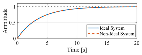
Figure 17.
Leg-balancing controller response.
5.5. Arm-Balancing Control
We perform the same considerations highlighted in the leg-balance control; the current in the battery in the upper and lower arms can be calculated as follows:
is the component of the peak of the circulating current.
In addition, the battery SOCs of the lower and upper arms can be obtained as:
Therefore, the following transfer function is obtained:
where is given by:
In this system, a P controller is used. Then, the transfer function is given by:
The block diagram of the arm-balancing control is presented in Figure 18. The open-loop transfer function is given by:
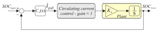
Figure 18.
Block diagram for arm-balancing control.
The closed-loop transfer function is represented by:
Analyzing , the closed-loop poles must be located in the left semi-plane for the system to be stable. In effect, the gain to adjust the proportional controller can be calculated as follows:
where is the location of the closed-loop pole. Thus, Figure 18 represents the block diagram for arm-balancing control.
The control strategy considers an internal loop of the circulating current with the fastest dynamics and the SOC external loop with the slower dynamics. The open-loop frequency response of the arm-balancing control is shown in Figure 19. Considering that the external loop has slower dynamics than the circulating current loop, the arm-balancing control is allocated to three decades of the circulating current control. According to the Bode diagram, the system has a gain margin of 76.2 dB at 4.05 kHz and a phase margin of 89.7 at 0.391 Hz. Comparing the frequency responses of ideal and non-ideal systems, we observe similar behaviors within the frequency range of the controllers.
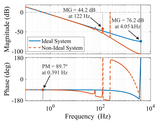
Figure 19.
Arm-balancing controller–open-loop Bode diagram.
The step response for the closed-loop transfer function comparing ideal and non-ideal systems is shown in Figure 20. Note that the behaviors of both systems are the same, and the system needs 2.5 s to reach the reference.
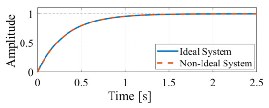
Figure 20.
Arm-balancing controller step response.
5.6. Individual SOC-Balancing Control
The block diagram of the individual SOC-balancing control is presented in Figure 21. The individual SOC-balancing control aims to reduce the difference between the reference SOC and the ith SOC converter SM. Consider , the difference between the average value of the SOC in an arm, and the value of the in the nth cell of the converter in the respective arm.
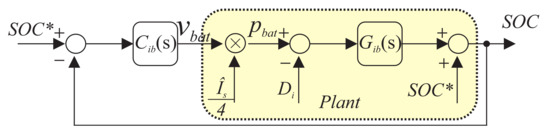
Figure 21.
Block diagram for the individual SOC-balancing control.
The value of can decrease the process of charging and discharging the battery in the SM battery of a given arm. For this process to take place properly, an AC voltage is superimposed to minimize the difference. The voltage can be calculated as follows:
where is a proportional gain. Note that the expression considers phase A. However, for the other phases, it can be applied without loss of generality.
The active power required to perform SOC balancing in a SM is given by:
where represents a loss or a disturbance in the converter cell. An active power, , is extracted or released from the SM in order to vary the SOC so that .
is a proportional controller. Furthermore, the plant transfer function of the individual SOC-balancing control is given by:
Therefore, the closed loop transfer function can be obtained as follows:
Finally, the transfer function has the function of rejecting disturbances. In fact, the project uses the dynamic stiffness method. Therefore, the proportional gain can be calculated as follows.
where is the location of the closed-loop pole.
Figure 22 shows the frequency response for the open-loop transfer function of the individual SOC-balancing control. The system has a gain margin of 44 dB at 1.35 kHz and a phase margin of −180 at 0 Hz.
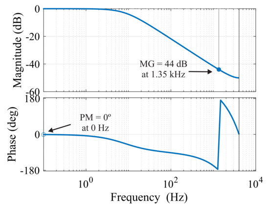
Figure 22.
Individual SOC-balancing controller–open-loop Bode diagram.
Figure 23 shows the step response for the closed loop of the individual SOC-balancing control. The system needs approximately 2.5 s to reach the unit reference.

Figure 23.
Individual SOC-balancing controller step response.
Table 3 presents a summary of the frequencies used to control the MMC-based BESS single-stage approach.
Table 3.
Frequency bandwidth for the MMC-based BESS.
Finally, the gains of the controllers used in the simulations for the single-stage approach are shown in Table 4.
Table 4.
Controller parameters of the MMC-based BESS.
6. Results
The PLECS simulations are used for evaluating the dynamics of the MMC-based BESS single-stage approach. In both approaches, they are evaluated in the process of the charge and discharge of the batteries.
6.1. Charging Procedure
For the battery-charging process, the simulation time is 220 s. In the beginning, the arm-balancing control is disabled. Then, at s, this controller is activated. To validate the SOC arm-balancing control, the upper arms of each phase start with 1% greater than those of the lower arm. At , a step in the SOC is applied from 52% to 55%. Furthermore, in the loading process, the leg-balancing control is deactivated, because the global SOC control is responsible for the balance of the battery SOC.
Figure 24a presents the SOC behavior in phase A and the average SOC for the three phases. The SOCs in the arm are not spread out and are within the tolerance range of 1%. Figure 24b shows the average SOC of the arms of each phase. As observed, before 20 s, there is no balancing of the arms. Afterward, the energy balance control is activated and the SOC average is balanced. Following the SOC reference step, the SOC of the battery increases following a ramp due to the active power limitation (1 pu). After 10 s, the batteries reach a steady state.
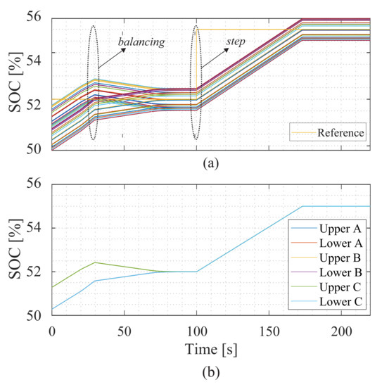
Figure 24.
SOC behavior during the charging process: (a) SOC phase A and (b) average SOC.
Active and reactive powers during the charging process are shown in Figure 25a. As observed, the reactive power is controlled to zero, while the active power is defined by the global SOC control. When the SOC reaches the reference value, the active power reduces to a value close to zero. Figure 25b shows the transient response at the SOC balancing instant and Figure 25c shows the transient response of the power outputs at the step instant.
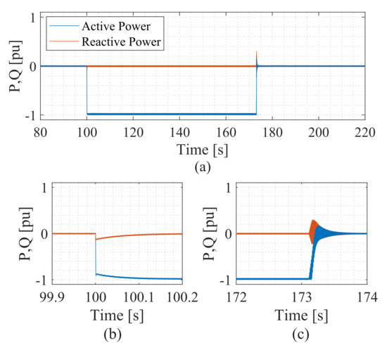
Figure 25.
Dynamic behavior during the battery charging process: (a) active and reactive power, (b) transient response at the balancing instant, (c) transient response at the step instant.
The grid current follows the behavior of the active power, as shown in Figure 26a. Figure 26b shows a zoomed-in view of the grid current, which is practically sinusoidal. The THD at this operating point is 0.1%. Figure 26c shows the transient response of the network current. Note that the response time is consistent with what is shown in Figure 8.
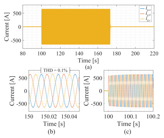
Figure 26.
The behavior of the grid current during the battery charging process: (a) grid current, (b) zoomed-in view of the grid current at the balancing instant, and (c) zoomed-in view of the grid current at the step instant.
As seen in Figure 24, before the SOC balance control operates, the current and the variation in the current reference of one phase affects the others, as shown in Figure 27a. Due to imbalances between the SOC, a 60 Hz component is observed in the circulating current. Finally, Figure 27c shows a zoomed-in view of the circulating current in a steady state. As expected, when the SOC balancing is reached, the AC circulating current goes to zero and only the ripple is observed.
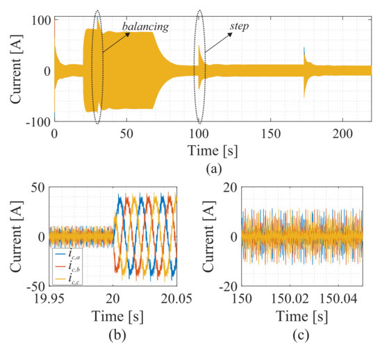
Figure 27.
Dynamic behavior of the circulating current during the charging process: (a) circulating current; (b) zoomed-in view of the transitory state; (c) zoomed-in view of the steady state.
6.2. Discharge Procedure
In the battery discharge process, the simulations started with the same initial conditions as the previous tests. However, for the discharge process, the global SOC control is disabled, while the leg-balancing control is enabled. At s, the negative step is applied after the system reaches the steady state. Therefore, the grid current reference is computed based on Equation (15).
Figure 28 shows the behavior of the SOC of the MMC-based BESS in the battery discharge process. The individual SOC of phase A maintains the same behavior presented in the discharge process. Because the SOC control is disabled, small mirroring can be seen in the average SOC of the converter; Figure 28b.
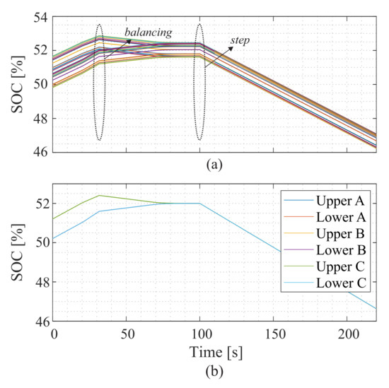
Figure 28.
SOC behavior during the discharging process: (a) SOC phase A and (b) average SOC.
Figure 29a shows the dynamic behavior of the instantaneous active power injected into the grid for the single-stage approach. As observed, the converter injects 1 pu of active power during the discharge process. In Figure 29b, one can see a zoom-in of the transients of the active and reactive powers. Figure 29c presents the output’s current response. As noted in Figure 29d, during the battery discharge, the peak current is, approximately, 600 A. Por fim, na Figure 29d presents the grid currents during the instant that the system is in a steady state.

Figure 29.
Dynamic behavior during the battery discharging process: (a) active and reactive power, (b) transient of active and reactive power at the start of discharge, (c) grid current, (d) three-phase grid current and (e) grid current zoom at steady state instant.
Figure 30a shows the current behavior during the charging process for the single-stage approach. Analyzing the current spectrum in Figure 30c, low-frequency components with high amplitudes are observed. The fundamental and secondary harmonic components are the most significant in the battery current’s harmonic spectrum. Finally, there is a scattering of harmonic components; this is justified by the fact that the batteries are connected directly to the SM without any type of filter.
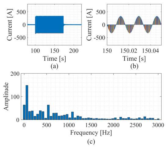
Figure 30.
Current in the batteries for the single-stage approach: (a) dynamic behavior, (b) current in the charging process, (c) spectral analysis.
6.3. Charging Procedure-Active and Reactive Power
In this simulation, the reactive power control is evaluated through a step during battery charging. The simulation lasts for 120 s. The active power in the simulation is 0.5 pu. At 85 s, a step in the reactive power from 0 pu to 1 pu is performed. Figure 31a shows the behavior of the SOC in phase A and Figure 31b shows the average behavior of the SOC for the three phases.
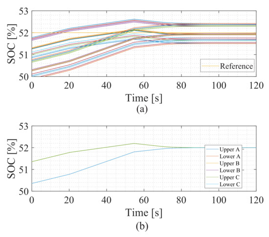
Figure 31.
SOC behavior during the charging process to the reactive power step: (a) phase A SOC and (b) average SOC.
Figure 32a shows the dynamics of the active and reactive power during the battery charging process. Initially, the active power is equal to 0.5 pu and goes to 0 pu when the SOC is equalized. The reactive power starts at 0 pu and goes to 1 pu after 85 s. Figure 32b shows the response time during SOC equalization and Figure 32c shows the response for the reactive power step. After the reactive power step, the active power presents a steady-state negative value. This is observed because the grid provides the converter energy losses.
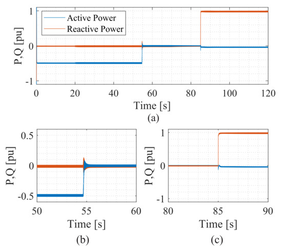
Figure 32.
Dynamic behavior during the step reactive power: (a) active and reactive power, (b) transient response at the balancing instant, (c) transient response at the step instant.
Figure 33a shows the behavior of the grid current during the battery charging process. Figure 33b shows a zoomed-in view of the current system reaching a steady state; Figure 33c shows the behavior of the grid current at the instant of the reactive power step.
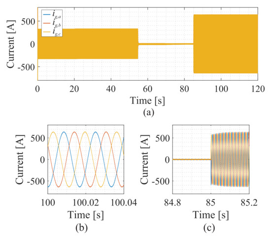
Figure 33.
The behavior of the grid current during the reactive power step: (a) grid current, (b) zoomed-in view of the grid current at the balancing instant, and (c) zoomed-in view of the grid current at the step instant.
Figure 34a shows the behavior of the circulating current in the battery charging process. Note that during the SOC balance process and in the reactive power step, disturbances in the behavior of the circulating current are observed. However, the response time is fast and consistent with the designed control loop. Figure 34b displays the behavior of the circulating current during the step process in reactive power. Finally, Figure 34c shows a zoomed-in view of the circulating current at a steady state.
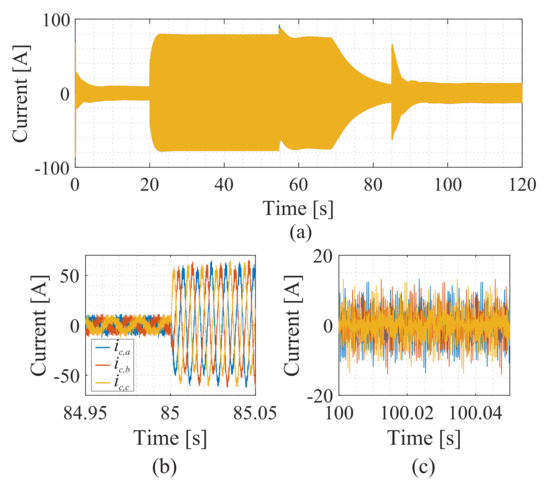
Figure 34.
Dynamic behavior of the circulating current during the reactive power step: (a) circulating current; (b) zoomed-in view of the transitory state; (c) zoomed-in view of the steady state.
7. Conclusions
This paper discusses a control strategy and how to perform control tuning for the MMC-based BESS. Thus, a control-tuning strategy and a methodology are presented to obtain the gains for each controller. The control strategies were designed for the single stage. In addition, this control methodology applies to different battery models/chemistry.
The methodology used to calculate controller gains is based on pole allocation. In a system with many control loops, this strategy makes it possible to minimize interference between the loops. Among the control loops discussed, one approach involves the use of independent control of energy levels in each arm. The decoupling of the system allows for a better balance of the SOC between the arms.
To validate the controls and gains obtained, the frequency response was presented through the Bode plot and the step response. Next, completing the validation of the controllers, the MMC-based BESS converter in the single-stage approach was simulated using PLECS software. The results pertain to the moments of charge and discharge of the batteries. As shown in the results, MMC-based BESS presented satisfactory dynamics.
Author Contributions
Conceptualization, J.H.D.G.P., A.F.C., H.A.P. and S.I.S.J.; Investigation, S.I.S.J.; Methodology, J.H.D.G.P., A.F.C., H.A.P. and S.I.S.J.; Resources, J.H.D.G.P., A.F.C., H.A.P. and S.I.S.J.; Writing—original draft, J.H.D.G.P., A.F.C., H.A.P. and S.I.S.J.; Writing—review & editing, J.H.D.G.P., A.F.C., H.A.P. and S.I.S.J. All authors have read and agreed to the published version of the manuscript.
Funding
This research was funded by CNPq (Grant 408058/2021-8), and FAPEMIG (Grant APQ-02556-21).
Acknowledgments
The authors thank the Brazilian agencies CAPES, National Council for Scientific and Technological Development-CNPq (Grant 408058/2021-8), and FAPEMIG (Grant APQ-02556-21) for the funding.
Conflicts of Interest
The authors declare no conflict of interest.
References
- Qiu, S.; Shi, B. An enhanced battery interface of MMC-based BESS. In Proceedings of the 2019 IEEE 10th International Symposium on Power Electronics for Distributed Generation Systems (PEDG), Xi’an, China, 3–6 June 2019; IEEE: Piscataway, NJ, USA, 2019; pp. 434–439. [Google Scholar]
- Puranik, I.; Zhang, L.; Qin, J. Impact of low-frequency ripple on lifetime of battery in MMC-based battery storage systems. In Proceedings of the 2018 IEEE Energy Conversion Congress and Exposition (ECCE), Portland, OR, USA, 23–27 September 2018; IEEE: Piscataway, NJ, USA, 2018; pp. 2748–2752. [Google Scholar]
- Ma, Y.; Lin, H.; Wang, Z.; Wang, T. Capacitor voltage balancing control of modular multilevel converters with energy storage system by using carrier phase-shifted modulation. In Proceedings of the 2017 IEEE Applied Power Electronics Conference and Exposition (APEC), Tampa, FL, USA, 26–30 March 2017; IEEE: Piscataway, NJ, USA, 2017; pp. 1821–1828. [Google Scholar]
- IEA. Total Installed Battery Storage Capacity in the Net Zero Scenario, 2015–2030; IEA: Paris, France, 2021. [Google Scholar]
- Abuagreb, M.; Allehyani, M.; Johnson, B.K. Design and test of a combined pv and battery system under multiple load and irradiation conditions. In Proceedings of the 2019 IEEE Power & Energy Society Innovative Smart Grid Technologies Conference (ISGT), Washington, DC, USA, 18–21 February 2019; IEEE: Piscataway, NJ, USA, 2019; pp. 1–5. [Google Scholar]
- Pinto, J.H.D.G.; Amorim, W.C.S.; Cupertino, A.F.; Pereira, H.A.; Junior, S.I.S. Benchmarking of Single-Stage and Two-Stage Approaches for an MMC-Based BESS. Energies 2022, 15, 3598. [Google Scholar] [CrossRef]
- Xavier, L.S.; Amorim, W.; Cupertino, A.F.; Mendes, V.F.; do Boaventura, W.C.; Pereira, H.A. Power converters for battery energy storage systems connected to medium voltage systems: A comprehensive review. BMC Energy 2019, 1, 7. [Google Scholar] [CrossRef]
- Ota, J.I.Y.; Sato, T.; Akagi, H. Enhancement of performance, availability, and flexibility of a battery energy storage system based on a modular multilevel cascaded converter (MMCC-SSBC). IEEE Trans. Power Electron. 2015, 31, 2791–2799. [Google Scholar] [CrossRef]
- Zhang, L.; Gao, F.; Li, N.; Zhang, Q.; Wang, C. Interlinking modular multilevel converter of hybrid AC-DC distribution system with integrated battery energy storage. In Proceedings of the 2015 IEEE Energy Conversion Congress and Exposition (ECCE), Montreal, QC, Canada, 20–24 September 2015; IEEE: Piscataway, NJ, USA, 2015; pp. 70–77. [Google Scholar]
- Pinto, J.H.D.G.; Amorim, W.C.S.; Cupertino, A.F.; Pereira, H.A.; Junior, S.I.S.; Teodorescu, R. Optimum Design of MMC-Based ES-STATCOM Systems: The Role of the Submodule Reference Voltage. IEEE Trans. Ind. Appl. 2020, 57, 3064–3076. [Google Scholar] [CrossRef]
- Debnath, S.; Qin, J.; Bahrani, B.; Saeedifard, M.; Barbosa, P. Operation, control, and applications of the modular multilevel converter: A review. IEEE Trans. Power Electron. 2014, 30, 37–53. [Google Scholar] [CrossRef]
- Badreldien, M.M.; Chakhchoukh, Y.; Johnson, B.K. Modeling and Control of Wind Energy Conversion System with Battery Energy Storage System. In Proceedings of the 2021 North American Power Symposium (NAPS), College Station, TX, USA, 14–16 November 2021; pp. 1–6. [Google Scholar] [CrossRef]
- Chaudhary, S.K.; Cupertino, A.F.; Teodorescu, R.; Svensson, J.R. Benchmarking of modular multilevel converter topologies for ES-STATCOM realization. Energies 2020, 13, 3384. [Google Scholar] [CrossRef]
- Wang, G.; Konstantinou, G.; Townsend, C.D.; Pou, J.; Vazquez, S.; Demetriades, G.D.; Agelidis, V.G. A review of power electronics for grid connection of utility-scale battery energy storage systems. IEEE Trans. Sustain. Energy 2016, 7, 1778–1790. [Google Scholar] [CrossRef]
- Wersland, S.B.; Acharya, A.B.; Norum, L.E. Integrating battery into MMC submodule using passive technique. In Proceedings of the 2017 IEEE 18th Workshop on Control and Modeling for Power Electronics (COMPEL), Stanford, CA, USA, 9–12 July 2017; IEEE: Piscataway, NJ, USA, 2017; pp. 1–7. [Google Scholar]
- Soong, T.; Lehn, P.W. Evaluation of emerging modular multilevel converters for BESS applications. IEEE Trans. Power Deliv. 2014, 29, 2086–2094. [Google Scholar] [CrossRef]
- Li, N.; Gao, F.; Hao, T.; Ma, Z.; Zhang, C. maharjan2009state Balancing Control Method for the MMC Battery Energy Storage System. IEEE Trans. Ind. Electron. 2018, 65, 6581–6591. [Google Scholar] [CrossRef]
- Vasiladiotis, M.; Rufer, A. Balancing control actions for cascaded H-bridge converters with integrated battery energy storage. In Proceedings of the 2013 15th European Conference on Power Electronics and Applications (EPE), Lille, France, 2–6 September 2013; IEEE: Piscataway, NJ, USA, 2013; pp. 1–10. [Google Scholar]
- Cupertino, A.F.; Amorim, W.C.S.; Pereira, H.A.; Junior, S.I.S.; Chaudhary, S.K.; Teodorescu, R. High performance simulation models for ES-STATCOM based on modular multilevel converters. IEEE Trans. Energy Convers. 2020, 35, 474–483. [Google Scholar] [CrossRef]
- Vasiladiotis, M.; Rufer, A. Analysis and control of modular multilevel converters with integrated battery energy storage. IEEE Trans. Power Electron. 2014, 30, 163–175. [Google Scholar] [CrossRef]
- Bin, R.; Yonghai, X.; Qiaoqian, L. A control method for battery energy storage system based on MMC. In Proceedings of the 2015 IEEE 2nd International Future Energy Electronics Conference (IFEEC), Taipei, Taiwan, 1–4 November 2015; IEEE: Piscataway, NJ, USA, 2015; pp. 1–6. [Google Scholar]
- Sharifabadi, K.; Harnefors, L.; Nee, H.; Norrga, S.; Teodorescu, R. Dynamics and Control. In Design, Control, and Application of Modular Multilevel Converters for HVDC Transmission Systems; John Wiley & Sons: Hoboken, NJ, USA, 2016; pp. 133–213. [Google Scholar]
- Millman, J. A Useful Network Theorem. Proc. IRE 1940, 28, 413–417. [Google Scholar] [CrossRef]
- Chiew, J.; Chin, C.; Toh, W.; Gao, Z.; Jia, J.; Zhang, C. A pseudo three-dimensional electrochemical-thermal model of a cylindrical LiFePO4/graphite battery. Appl. Therm. Eng. 2019, 147, 450–463. [Google Scholar] [CrossRef]
- Perez, M.A.; Ceballos, S.; Konstantinou, G.; Pou, J.; Aguilera, R.P. Modular Multilevel Converters: Recent Achievements and Challenges. IEEE Open J. Ind. Electron. Soc. 2021, 2, 224–239. [Google Scholar] [CrossRef]
- Tsolaridis, G.; Kontos, E.; Chaudhary, S.K.; Bauer, P.; Teodorescu, R. Internal balance during low-voltage-ride-through of the modular multilevel converter STATCOM. Energies 2017, 10, 935. [Google Scholar] [CrossRef]
- A123 Systems. A123 Systems Nanophosphate High Power Lithium Ion Cell ANR26650m1-b. 2012. Available online: http://www.a123systems.com/ (accessed on 25 January 2023).
- Yao, W.; Yang, Y.; Zhang, X.; Blaabjerg, F.; Loh, P.C. Design and Analysis of Robust Active Damping for LCL Filters using Digital Notch Filters. IEEE Trans. Power Electron. 2017, 32, 2360–2375. [Google Scholar] [CrossRef]
- Han, Y.; Yang, M.; Li, H.; Yang, P.; Xu, L.; Coelho, E.A.A.; Guerrero, J.M. Modeling and Stability Analysis of LCL -Type Grid-Connected Inverters: A Comprehensive Overview. IEEE Access 2019, 7, 114975–115001. [Google Scholar] [CrossRef]
Disclaimer/Publisher’s Note: The statements, opinions and data contained in all publications are solely those of the individual author(s) and contributor(s) and not of MDPI and/or the editor(s). MDPI and/or the editor(s) disclaim responsibility for any injury to people or property resulting from any ideas, methods, instructions or products referred to in the content. |
© 2023 by the authors. Licensee MDPI, Basel, Switzerland. This article is an open access article distributed under the terms and conditions of the Creative Commons Attribution (CC BY) license (https://creativecommons.org/licenses/by/4.0/).