Review

Navier-Stokes Solutions for Accelerating Pipe Flow—A Review of Analytical Models

1
Faculty of Mechanical Engineering and Mechatronics, West Pomeranian University of Technology in Szczecin, 70-310 Szczecin, Poland
2
Litostroj Power d.o.o., 1000 Ljubljana, Slovenia
3
Faculty of Mechanical Engineering, University of Ljubljana, 1000 Ljubljana, Slovenia
4
Faculty of Mechanical Engineering, Wrocław University of Science and Technology, 50-370 Wrocław, Poland
5
Faculty of Production Engineering and Logistics, Opole University of Technology, 45-758 Opole, Poland
6
Faculty of Transport Engineering, Vilnius Gediminas Technical University, LT-10223 Vilnius, Lithuania
*
Author to whom correspondence should be addressed.
Energies 2023, 16(3), 1407; https://doi.org/10.3390/en16031407
Submission received: 30 November 2022 / Revised: 5 January 2023 / Accepted: 20 January 2023 / Published: 31 January 2023
(This article belongs to the Special Issue Numerical Heat Transfer and Fluid Flow 2022)

Abstract

:
This paper reviews analytical solutions for the accelerated flow of an incompressible Newtonian fluid in a pipeline. This problem can be solved in one of two ways according to the (1) imposed pressure gradient or (2) flow rate. Laminar accelerated flow solutions presented in a number of publications concern cases where the two driving mechanisms are described by simple mathematical functions: (a) impulsive change; (b) constant change; (c) ramp change, etc. The adoption of a more complex and realistic description of the pressure gradient or flow rate will be associated with a profound mathematical complexity of the final solution. This is particularly visible with the help of the universal formula derived by several researchers over the years and discussed in this paper. In addition to the solutions strictly defined for laminar flow, an interesting extension of this theory is the theory of underlying laminar flow for the analysis of turbulent accelerated pipe flows (TULF model developed by García García and Alvariño). The TULF model extends the Pai model developed more than 60 years ago, which has been previously used for steady flows only. The discussed solutions extend the theory of analytical solutions of simplified two-dimensional Navier–Stokes equations and can be used not only to study the behavior of liquids during accelerating pipe flow but they can also be used to test the accuracy of commercial CFD codes.

Graphical Abstract

1. Introduction

Fluid flow in hydraulic pipes is often time-varying flow. This means that the basic parameters of the flow, i.e., the average value of velocity and pressure in the analyzed pipe cross-section, dynamically change over time. Time-varying flows can be accelerated, decelerated, reverse, pulsating, oscillating and water hammer-type flows. This paper reviews analytical models for accelerating pipe flows.
Starting with the work of Navier [1], the basic hydrodynamic equations (according to the work of Darrigoll [2], these have been re-derived at least four times chronologically by the following well-known researchers: Cauchy, Poisson, Saint-Venant and Stokes), are the subject of numerous studies. Analyzing the literature on analytical solutions of laminar accelerated flows, it can be seen that two groups of flows can exist [3,4]: the first is flows forced by the occurrence of a step pressure gradient change, while the second group of flows is those in which the fluid movement is forced by a step change in the flow rate.
Much earlier, solutions from the first group were analyzed, i.e., when the flow is forced by a change of the pressure gradient along the length of the pipe. The oldest paper found for this review was published by the Italian scientist Roiti [5] in 1871, who worked at the University of Pisa. He studied accelerated flow in a simple vertical water system. The pressure change was obtained by rapidly opening the valve. Apart from experimental research, Roiti’s most important achievement was the presentation of an analytical theory of this flow. This referred to solutions previously described by another researcher from the University of Pisa, namely Betti [6], who analyzed heat flows. Another important work was written in 1882 by Gromeka [7]. Unfortunately, due to the fact that it was published only in Russian, it remains known mainly among authors of Russian origin [8,9,10,11], who mostly know it from an important reprint of all Gromeka’s works in a book form, published on the 100th anniversary of his birth [12]. It was only thanks to the work of Szymański [13] published in 1932 in a respected French mathematical journal (Journal de Mathématiques Pures et Appliquées—still existing and new papers being published) that this solution was noticed and reproduced in many books on the flow of viscous fluids [14,15,16]. The accelerated solution forced by a rapid, strictly defined pressure gradient was then analyzed by a number of researchers who extended its applicability. Among these studies, the work of Gerbes [17], was the first to apply the Laplace transform to its derivation, should be noted, as well as that of Ito [18], who extended the scope of this solution to make it suitable for the analysis of unsteady transient flows occurring between one steady flow (of the Hagen–Poiseuille type) and another characterized by a higher average velocity.
For short pipes, the entrance length plays an important role. Solutions for this unsteady acceleration problem devoted to the development of the velocity profile along the pipe length and in time have been derived by Atabek [19] and Avula [20]. Fan [21] solved the problem of accelerated flow in rectangular ducts. Solutions in ducts with an arbitrary geometry were the subject of research by Laura [22]. This issue has been recently analyzed by Muzychka-Yovanovich [23,24] as well. In the following years, similar solutions were developed for non-Newtonian fluid flows [25,26,27,28] for which the shearing stress is not linearly related to the rate of shearing strain [29].
The second group of models, i.e., those in which the function of velocity or flow rate is defined in the main equation of motion, has been analyzed since 1933, when Vogelpohl’s short technical note was published [30]. In his note, Vogelpohl also mentioned the experimental research carried out at the University of Berlin by Prof. Föttinger on accelerated flows. In addition, he derived a formula (using the Whittaker method [31]) for the time-varying pressure gradient for this type of flow (later re-derived by Andersson and Tiseth [32]) for a constant value of average velocity. Other researchers who were interested in this type of flow were Weinbaum and Parker [33], although their interest was mostly focused on the decelerated flow resulting from the sudden closing of the gate valve. Weinbaum and Parker’s research was the inspiration for subsequent works, including the work of Andersson and Tiseth [32], which is particularly important from the point of view of this review. It was in this work that for the first time a complete analytical solution for the flow velocity profile was derived for a constant mean velocity scenario that can be the effect of piston movement. It should be mentioned here that Andersson and Kristoffersen [34] had previously analyzed a wide range of flows forced by a pressure gradient (RGS type) as well as the correction to this solution proposed by Otis [35]. The Anderson and Tiseth solution has been improved by Das and Arakeri [36], who presented analytical solutions for a complete piston cycle (acceleration period, motion with constant velocity, deceleration period and final period). The Das and Arakeri solutions for the first two periods (i.e., acceleration and piston work at constant velocity) can be treated as a complete solution when imposing a ramp-type motion. This solution was further refined by Kannaiyan et al. [37] by introducing the possibility of determining the transition from one steady state to another.
The main experimental studies that confirmed the correctness of the solution based on a step change in pressure were carried out by van de Sande et al. [38] and Lefebvre and White [39]. These studies show that laminar flow is maintained during acceleration for a relatively long time—in the paper by van de Sande et al. [38] to Re = 57,500, and in the work of Lefebvre and White [39] to Re > 105. This delayed transition from laminar to turbulent flow was also mentioned by Goldberg in a discussion on van de Sande et al. at the Pressure Surges Conference in Canterbury [38]. Goldberg (p. 499 of Pressure Surges 1980 proceedings) wrote about a long distant oil transportation pipeline (105 miles long, twenty inches in diameter) located in the Gulf of Mexico in which, during the start-up, a delayed transition to turbulent flow was detected.
As opposed to pressure-driven flows, the other type of acceleration occurs in systems due to a step change in flow rate, e.g., piston-driven flow. In an early experiment by Kataoka et al. [40], the measured results did not agree well with the theory as an annular jet effect was reported. The research, which indicated the correctness of the theoretical solution for a fixed flow rate, was carried out by a team led by Chaudhury et al. [41]. Recently He et al. [42] have reported that the whole acceleration phase in pipes is a laminar–turbulent bypass transition, so even during the initial flow, some turbulent structures that initially occupy the near wall region are present in the flow.
Although this paper concerns only accelerated Newtonian liquid flows in pipes with circular cross-sections (typical, commonly used in practice, Figure 1), the scope of research is very extensive. Readers interested in further solutions (flows through other cross-sections, accelerated flows of non-Newtonian fluids, etc.), which were developed on the basis of the accelerated flows theory discussed in this review, will be offered additional reading elsewhere.
In Section 2 and Section 3 of the present review paper, accelerating laminar flow solutions will be discussed. Laminar flow means that the orderly movement of the fluid along parallel paths occurs in which the fluid elements do not mix with each other, and there is, therefore, a purely viscous mechanism of momentum and energy exchange. Section 4 discusses a turbulent semi-analytical solution. Turbulent flow is understood as a chaotic motion of a fluid. During this flow the elements of the fluid mix with each other, which leads to the intensification of mass, momentum and energy exchange.

2. Accelerated Laminar Flows Driven by Pressure Gradient

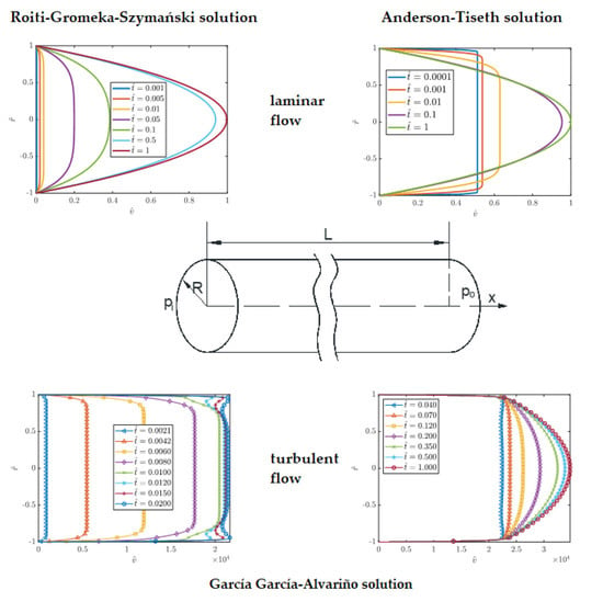
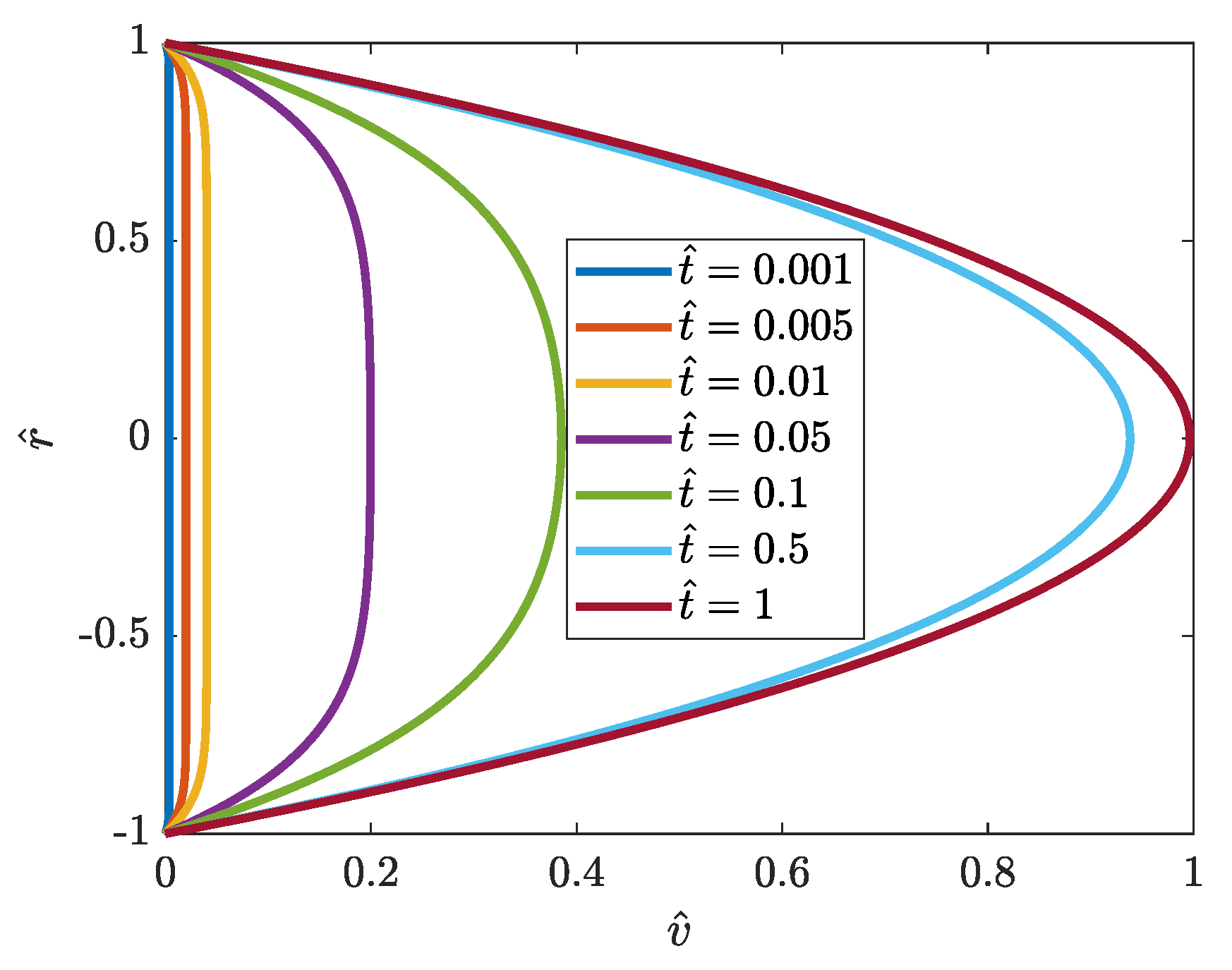
2.1. Rapid Instantaneous Increment of Pressure Gradient (Roiti-Gromeka-Szymański Solution)

As mentioned in the introduction, the accelerated flow of liquid in pipes (Figure 1) has been the subject of many studies. All the authors who successfully derived the final solution started from the dynamic equation of motion first derived by Navier [1]:
v t = 1 ρ p x + ν 2 v r 2 + 1 r v r     v t = G + ν r r r v r
They assumed the incompressibility of the liquid and that the velocity field is only dependent on the pipe radius and time v = v r , t . This means that the problem is simplified to isothermal flow in long, constant inner diameter pipelines, where the entrance effects can be neglected. Other boundary conditions are:
(a)
flow starts initially from rest:
v r , 0 = 0 ,
(b)
no-slip condition as viscous fluid in contact with a rigid wall will adhere to the wall due to the effects of viscosity [43]. In the analyzed problem, the solid pipe wall boundary velocity is assumed to be equal to zero:
v R , t = 0 ,
(c)
final velocity profile consistent with the parabolic Hagen–Poiseuille equation:
v r , = v m a x 1 r R 2 ,
where: v m a x = R 2 4 μ p x = Δ p L R 2 4 μ = G R 2 4 ν ; Δ p = p o p i , p o —outlet pressure, p i —inlet pressure. Maximal velocity occurs at the pipe axis ( r = 0 ) .
(d)
sudden imposition of a pressure gradient (Figure 2a):
G = 0   f o r   t < 0 G = G = 1 ρ Δ p L   f o r   t 0
The literature review in the Introduction indicates that the final solution was found a relatively long time ago by at least three authors. Roiti [5] studied theoretically and experimentally the unsteady flow of liquid inside a vertically fixed cylindrical pipe, with its gravitational outflow to the atmosphere. He carried out the integration of general formulas using the same method by which his senior colleague Prof. Betti [6] determined the temperature distribution acting on the cylinder. Roiti was the only researcher who, in addition to formulas for the flow velocity, also derived formulas for the displacement of fluid elements during this movement.
Another researcher dealing with this phenomenon, albeit excluding gravitational forces (flow in the horizontal duct), was Gromeka [7]. The work in which he derived the final solution for this type of flow was his doctoral thesis. Gromeka also based his derivation on the analogy existing between some problems related to the movement of viscous fluids and those known from the theory of heat conduction. He carefully used the method of solving heat distributions in circular cylinders proposed by Poisson in his dissertations on “Mémoire sur la distribution de la chaleur dans les corps solides” [44]. In addition to deriving the final formula for the velocity profile (for step gradient change Figure 2a), Gromeka proved that the flow which is forced by a pulsating pressure gradient also for large times tends towards the Hagen–Poiseuille flow. Gromeka also derived formulas for accelerated flow with possible slippage of liquid elements on the walls of the pipe. Both Gromeka’s and Roiti’s solutions remained unnoticed by the world of science for a long time, likely due to a combination of being published in scientific journals by the researchers’ home universities and the slow movement of information at this time. Over a hundred years ago, there was no internet, and materials of this type were not widely available (in contrast to today’s open-access papers). Interestingly, Roiti’s solution was not quoted in the work of Allievi [45] or that of other Italian (and non-Italian) researchers of unsteady flows, e.g., Fasso [46], Aresti [47].
Fifty years after the publication of Gromeka’s thesis, and sixty after the publication of Roiti’s work, this interesting topic was addressed by a young Polish researcher, Piotr Szymański, who had just defended his doctoral thesis. Szymański, unaware of the work of his predecessors, during a one-year training course in Paris in 1928, applied the theory of the Fourier–Bessel series to find an analytical solution to this problem. In addition, after deriving the final formula, he conducted a number of mathematical studies on the continuity of its derivatives (using Abel transformations). It is worth mentioning that Szymański in his work [13] analyzed, similarly to Gromeka, the pulsating nature of the flow, and this took place long before Womersley or Uchida’s work. In the case of pulsating flow, Szymański analyzed the derivatives of the presented general solution of this problem with the help of the Fourier series theory as well as on the basis of M. Lebesque’s theorem. Like Gromeka, however, he did not define the final solution to this problem, which is known today. It is also worth adding here that Szymański’s main work was preceded by the publication of a conference paper of the 3rd International Congress of Applied Mechanics held in Stockholm in 1930 [48]. Among the distinguished participants of this congress was Theodore von Kármán.
Due to the fact that the analyzed solution, as can be seen from the above discussion, was derived independently by three researchers, it is suggested to define this solution with the abbreviation RGS derived from the first letters of the surnames of the authors. Leaving aside the tedious details of the derivations, the final solution of the system of Equation (1), assuming a step change in pressure, is the following function:
v r , t R G S = v m a x 1 r R 2 8 n = 1 J 0 λ n r R λ n 3 · J 1 λ n e λ n 2 ν R 2 t ,
where λ n are the nth zero, or root, of a Bessel function J 0 λ n .
An exemplary flow that develops according to the RGS solution described by Equation (6) is presented in Figure 3.
Gerbes in the 1950s [17] developed the same accelerated solution with help of the Laplace technique; in his work, he also presented a solution for decelerated flow as well as a solution for pulsating flow. The generalization of Equation (6) for the vertical (upward and downward) as well as arbitrary sloping pipes was presented recently by Urbanowicz et al. [49]. The maximal velocity for this case depends on the pipe slope angle β as follows (Figure 4):
v m a x = R 2 4 μ L Δ p g ρ L sin β .
From Equation (7), it follows that in the case of upward vertical flow where β = 90 ° :   v m a x = R 2 4 μ L Δ p g ρ L , while in the case of downward vertical flow where β = 90 ° , the maximal final velocity has the largest possible value equal to v m a x = R 2 4 μ L Δ p + g ρ L sin β .
Knowing the solution for velocity distribution at the pipe cross–section (Equation (6)) enables us to calculate the following important parameters describing unsteady accelerated pipe flow:
(a)
average flow velocity: v m = 2 R 2 0 R r v r , t d r
(b)
wall shear stress: τ w = μ v r , t r r = R
(c)
friction factor: f = 8 τ w ρ v m 2
The final form for the RGS-type accelerated flow is [49]:
v m ,   R G S = v 1 32 n = 1 e λ n 2 t ^ λ n 4 τ w , R G S = 4 μ v R 1 4 n = 1 e λ n 2 t ^ λ n 2 f R G S = 64 R e 1 4 n = 1 e λ n 2 t ^ λ n 2 · 1 32 n = 1 e λ n 2 t ^ λ n 4 2
Ito [18] generalized the above solution for the case where the initial velocity of the fluid is not zero, which means a steady Hagen–Poiseuille flow is a starting point, and next an instantaneous pressure gradient change takes place from an initial value equal G 0 to a new final value G (Figure 2b). In this case, the final solution is steady-state Hagen–Poiseuille flow but represented with a higher maximal velocity (in the axial position). The analytical solution obtained for this extended case is:
v r , t R G S I = G R 2 r 2 4 ν 2 R 2 G G 0 ν n = 1 J 0 λ n r R λ n 3 · J 1 λ n e λ n 2 ν R 2 t
The RGS analytical solution was initially verified experimentally by Letelier and Leutheusser [50] and in more detail by van de Sande et al. [38], Baibikov et al. [8] and Lefebvre and White [39]. In all the mentioned experimental works, good agreement between the RGS solution and the experimental results was indicated. As it is known from the standard textbooks on steady pipe flow, the critical Reynolds number is about 2320 [14]. Below this value laminar flow takes place. For Reynolds numbers of up to 3000, transitional flow occurs, and above that value, turbulent flow can be assumed. Lefebvre and White [39] noticed that the laminar flow persisted in their experimental runs up to very high values of Reynolds numbers in the range between 2 · 10 5 and 5 · 10 5 . In another study by van de Sande et al. [38], a lower value (Re = 57,500) was found. In both cases, however, it can be seen that the values of the critical Reynolds number exceeded the critical one in steady-state flow. From a paper that is a continuation of the Lefebvre and White study [51], a transitional Reynolds number formula has been proposed R e t 450 D a / ν 2 1 / 3 , in which a is acceleration, which was constant during experiments. A different formula based on the Knisely et al. experiments [52] is R e t 1.33 D a / ν 2 1 / 3 1.86 .

2.2. Other Solutions Driven by a Gradient Change

Ito [18], in addition to extending the RGS solution of Equation (9), has developed the solution for the case when the pressure gradient given to a pipe begins to increase or decrease in proportion to the time (gradient change scenario from Figure 2c):
t < 0   t h e n   1 ρ Δ p L = G 0 t 0   t h e n   1 ρ Δ p L = ε t + G 0 .
The final analytical solution in the Ito (I) case is:
v I = ε t + G 0 R 2 r 2 4 ν ε R 2 r 2 3 R 2 r 2 64 ν 2 + 2 R 4 ε ν 2 n = 1 J 0 λ n r R λ n 5 J 1 α n e λ n 2 ν R 2 t .
There is a problem with the above equation regarding how the value of ε function shall be calculated. The analysis of this equation shows that the lower the value of the ε coefficient (representing jerk as its unit is [m/s3]), the smaller the angle of inclination of the increasing gradient time curve, which will physically mean a larger time required to obtain the selected reference average value of the flow velocity.
The review of analytical solutions in this group revealed that among all derived analytical solutions, there is not one in which the ramp pressure gradient change is gradual, as shown in Figure 2d. Such a solution seems desirable because in practice there are no technical possibilities to change the pressure gradient in an instant way (for example, the valve opening time in the work of van de Sande et al. was about 0.1 s). In real systems, the change of pressure gradient will be strongly related to the valve opening time.
Avula [53] and Avula and Young [54] indicated that changes in velocity during accelerating flows in real systems occur differently than described by the above classical RGS theory. During their research, they experimentally recorded the pressure gradient histories (for selected values of Reynolds numbers—see Figure 5), then they described their mathematical form in an approximate way:
f t A = 1 2 d p d x ^ = a 1 1 e a 2 t A + a 3 t A a 4 e a 5 t A .
where a1,…, a5 are constants calibrated with the reference to experimental results and x ^ , p   and   t A are the normalized axial coordinate, pressure and time, respectively.
The final modified semi-analytical Avula’s solution for the velocity profile is:
v = 2 n = 1 J 0 η n r R η n 3 · J 1 η n { a 1 R e 2 η n 2 1 e x p 2 η n 2 R e t A + a 1 R e a 2 R e 2 η n 2 e a 2 t A e 2 η n 2 R e t A + a 3 e 2 η n 2 R e t A 0 t A u a 4 e   a 5 u + 2 η n 2 R e u d u } ,
where dimensionless time t A = t v m , R , v m , = R 2 8 μ p x = Δ p L R 2 8 μ is the final steady-state mean velocity and η n is a consecutive zero of a Bessel function of zero order J 0 s R e / 2 = 0 .
As the third right-hand side term of this solution (Equation (13)) cannot be evaluated explicitly, this solution needed to be evaluated partially numerically. This numerical solution significantly limits its practical application. A different mathematical form of the function f t A to describe changes in the pressure gradient over time should be found. Such a new function should be integrable to give a complete analytical solution for a wide range of final Reynolds numbers. Illustrative comparisons of the results obtained with the classical RGS model and Avula’s solution are shown in Figure 6 and Figure 7.
It can be seen from the comparisons in Figure 6 and Figure 7 that a large discrepancy in the profile dynamics is noticeable for small values of the dimensionless time t A < 10 , while for larger values t A > 200 , the Avula solution begins to catch up with the classical RGS solution.
A similar solution to the above was analyzed by Smith [55], who in his derivation referred to some of the solutions discussed in the classical textbook “Hydrodynamics” by Dryden et al. [56]. Smith’s solution was obtained for the following pressure gradient:
p x = b μ k 2 e ν k 2 t ,
where k and b are positive constants and μ and ν are the dynamic and kinematic viscosities, respectively. The final Smith’s (SM) solution is as follows:
v r , t S M = b 1 J 0 k r J 0 k R e ν k 2 t + 2 b k 2 n = 1 J 0 λ n r R e λ n 2 ν R 2 t λ n λ n 2 R 2 k 2 J 1 λ n .
When deriving the above solution, it was assumed that the pressure gradient appears at time t = 0 and then gradually decays exponentially to zero (and not to a constant value). Such a flow cannot be treated strictly as accelerated as two different periods occur. Firstly, liquid accelerates until the fluid reaches the maximal mean velocity, while after that it starts to decelerate until it comes back to rest again. That is why it is not a subject of the present review. However, this analytical solution is presented and discussed shortly, mainly because it has an interesting feature when the forced decay rate is equal to one of the natural decay rates. It is analogous to the feature experienced in the classical problem regarding oscillations of a linear pendulum in the case when the forcing frequency is equal to the natural frequency (there are two distinct singularities in this final solution).
Other problems with the accelerated pipe flow solution of the RGS type have been reported by Otis [35]. This author noticed that, usually, the pressure gradient does not remain constant but rather it is the total head H i , which is schematically presented in Figure 8.
During a flow acceleration, some portion of this head is utilized to establish the kinetic head of the flow. The above is illustrated in Figure 8 in which there are three energy grade lines: (a) just after the instantaneous valve opening, (b) at a later time and (c) after reaching steady-state flow (Hagen–Poiseuille steady state). During flow development, the pressure gradient along the pipe is diminished because of the observed velocity head development. With the above in mind, the main Navier equation becomes non-linear and it is necessary to use numerical methods to model it. Otis [35] presented experimental results (of accelerated flow) of an unnamed researcher and a realistic numerical example of a start-up for SAE 10W-30 oil driven by a head of 1.053 m in a 10-cm diameter pipe with a length of 6.25 m. The main conclusions were that the final steady-flow will occur in less than half the time predicted by the RGS solution. In the same paper, Otis developed a start-up parameter in the following form:
M G 0 D 4 2048 ν 2 ρ L ,
where G 0 = γ H i / L . Otis concluded that analysis of this parameter revealed that when M < 1, the wall shear stress rises monotonically with time, while for M > 1, the shear stress overshoots the steady-state value. In addition, Otis stated: “Such behavior resulting from the fact that the time constant for flow start-up decreases with M, whereas the time constant for boundary layer growth is independent of M.” Otis’s correction was verified numerically by Singh [57], who derived a corrected equation that he did not solve analytically but led to a numerical form suitable for the creation of a computer program and succeed numerical calculations. Patience and Mehrota [58] wrote the Otis start-up parameter in a much simpler form:
M R e · D 64 L
They also noted that both Szymański [13] and Otis [35] overlooked the hydrodynamic developing region effect in their works. Additionally, Patience and Mehrota proved that in the analyzed comparison start-up cases by Otis, the flow was not fully developed. Their conclusion was based with help of the Fargie and Martin ξ coefficient [59]. Andersson and Kristoffersen also dealt with this problem. In [34], they demonstrated that the start-up flow Otis parameter M defined by Equation (16) is the crucial parameter also when the entrance effects are taken into account. For long pipes (M = 0), the Anderson and Kristoffersen numerical solution differs by less than 1% from the exact analytic solution obtained by RGS. For shorter pipes, these authors observed that the start-up period and the resulting steady-state flow rate are significantly reduced due to the entrance region effects. When M = 0.5 the start-up time and ultimate flow rate are reduced by about 55% and 40%, respectively, compared with the classical solution of RGS derived for long pipes. In view of the above comments and discussed works, Patience and Mehrota [60] introduced a correction of the method proposed by Otis.

2.3. Universal Solution for Arbitrary Pressure Gradient

The analysis of a number of scientific papers for the purposes of this review revealed that there is a universal solution that can be used to determine the velocity profile for any change in the pressure gradient. Information about this solution will be the topic of this subsection.
Fan in his Ph.D. thesis [61] derived analytical solutions for: (a) impulsive pressure gradient (here the pressure gradient is a function of Dirac delta function); (b) flow under a constant pressure gradient (analogous to RGS solution); (c) flow under a harmonically oscillating pressure gradient; (d) a general solution by superposition integrals and (e) a general solution by the transformation of the governing equation of motion to a homogeneous equation. The latter helped Fan to derive a final analytical solution for an accelerated flow in a pipe with a rectangular cross-section, which will not be discussed due to limited practical applications. The most important solution according to this subsection title is the general solution defined by superposition integral. Since the considered problem is linear, Fan noticed that the solution for any arbitrary f t can be obtained by one of the following superposition integrals:
v r , t = 0 t f u v ¯ 1 r , t u d u = 0 t f t u v ¯ 1 r , u d u ,
where: 1 ρ p x = f t and v ¯ 1 r ^ , t ^ = 2 n = 1 J 0 r ^ λ n λ n J 1 λ n e λ n 2 t ^ is the solution that Fan obtained for impulsive pressure gradient, or:
v r , t = f 0 v ¯ 2 r , t 0 t f u v ¯ 2 r , t u d u = 0 t f u v ¯ 2 r , t u t d u ,
where v ¯ 2 r , t is the RGS solution v ¯ 2 r , t = 1 4 ν R 2 r 2 8 R 2 n = 1 J 0 λ n r R λ n 3 · J 1 λ n e λ n 2 ν R 2 t .
The First Fan integral solution Equation (18) is of simple mathematical structure. The second solution (known as Duhamel’s integrals) is based on the more demanding RGS solution Equation (19). Both superposition solutions described by Equations (18) and (19) were derived for the case with the initial flow at rest (mean velocity equal to zero). A solution that takes into account the initial flow was derived by Daneshyar [62]. Daneshyar gives a solution for an arbitrary f(t), using the theory of integral transforms to solve the main Equation (1). He proved after Sneddon [63] that if ξ n is chosen to be a root of:
J 0 R ξ n = 0
then
0 R r 2 v r 2 + 1 r v r J 0 r ξ n d r = ξ n 2 v ¯
where
v ¯ = 0 R r v r , t J 0 r ξ n d r
is the finite Hankel transform of v . When both sides of Equation (1) are multiplied by r J 0 r ξ n and integrated (within the limits 0 to R ), the following ordinary differential equation is obtained for v ¯ :
d v ¯ d t + ν ξ n 2 v ¯ = f t 0 R r J 0 r ξ n d r = f t R ξ n J 1 R ξ n
The solution that satisfies the initial condition v ¯ ξ n , 0 = v ¯ 0 is:
v ¯ = 0 t f u R ξ n J 1 R ξ n e x p ν ξ n 2 t u d u + v ¯ 0
And, next, with the inversion theorem of finite Hankel transforms, a general solution is found to be:
v = v 0 + 2 R 2 n = 1 J 0 r ξ n J 1 R ξ n 2 v ¯ = v 0 + 2 R n = 1 J 0 r ξ n ξ n J 1 R ξ n 0 t f u e x p ν ξ n 2 t u d u
that is valid for an arbitrary pressure gradient (hidden under f t function).
It can be now noticed that substituting for R ξ n = λ n one gets ξ n = λ n / R , which, when inserted into the above formula, will reduce this solution to the following form:
v = v 0 + 2 n = 1 J 0 r R λ n λ n J 1 λ n 0 t f u e λ n 2 t u d u ,
In the special case of the above solution, v 0 can be treated as an initiation laminar flow profile of steady Hagen–Poiseuille type flow.
A careful literature review reveals that universal solutions of this type were derived many times. Chronologically, the earliest form of this solution was presented by Vogepohl in a short note published in 1933 [30]. Then in 1956, Roller, in his master’s thesis [64], noticed (similarly to Daneshyar about 15 years later) that the solution of the Navier momentum equation can be obtained with the use of the analogy to the temperature distribution in a cylindrical rod (defining the analogous boundary and initial condition) [63]. Zielke in his Ph.D. thesis [65] rederived Fan’s solution in the form of Equation (19) using Laplace transforms. Hersey and Song by using Laplace transforms [66], and Avula with the help of the Cauchy residue and convolution integral theorem [53], derived the same solution but based on different normalized quantities. These solutions were again derived and used with the help of the eigenfunction method in the work of Xiu et al. [67], where the starting flow was analyzed, and in the Sun and Wang paper [68], where the water hammer case (starting from steady Hagen–Poiseuille flow) was examined:
v ^ r ^ , x ^ , t ^ = n = 1 16 J 0 r ^ λ n λ n 3 J 1 λ n e λ n 2 t ^ + n = 1 0 t ^ 2 J 0 r ^ λ n λ n J 1 λ n H ^ x ^ , u x ^ e λ n 2 t ^ u d u
where: x ^ = x / L ; r ^ = r / R ; v ^ = v / v 0 and H ^ = Δ p R 2 L μ v 0 .
In the above equation, an interesting identity is used (for initial time t ^ = 0 ), that can be found in many papers among them the ones discussed in this review i.e., Szymański [13], Gerbes [17], Xiu et al. [67], etc:
n = 1 8 J 0 λ n r ^ λ n 3 J 1 λ n = 1 r ^   for   0 r ^ 1
The most recent study in which this universal equation was re-derived and examined is Lee’s paper published in 2017 in Applied Mathematical Modelling [69]. The motivation of this section is to systematize the derivation of the universal formula discussed above. The list of references is presented in Table 1.

2.4. Comments on the Pressure Gradient Driven Flows

As noticed, the formulas discussed above concerned pipes with circular cross-sections. Readers interested in other solutions, e.g., similar accelerated flow in ducts with different geometry, are referred to other works: the solution to this problem for ducts with a rectangular cross-section was derived in the works of Fan and Erdogan [21,61,72]; start-up flow in an annulus was developed by Müller [73]; for other cross-sections, an intensive study was carried out by Laura [22]; solution for pipes, taking into account the slip of the fluid on the wall [74]; start-up flow in a circular porous pipe [75]; development of unsteady flow at the entrance length of a circular tube starting from rest [19,20,54,76]; the effects of time-dependent viscosity [77,78,79]; unsteady laminar flow in tubes with a tapered wall thickness [80], etc.
Due to the need to use the zeros of the Bessel function, the presented solutions are a challenge, because it is usually necessary to write a short program in software such as Matlab or Wolfram Mathematica, hence the approximation forms of these formulas discussed by Muzychka-Yovanovich [23,24] and Urbanowicz et al. [4] are also an interesting proposition. It is also worth adding that governing equations of motion, are respectively analogous to heat conduction in a long cylinder with constant thermal conductivity [81]. So all the results presented in this paper for laminar flows are directly transformable to the solution of heat conduction in long cylinders with internal heat generation (simply replacing pressure gradient G by heat generation source term g ˙ c P · ρ ; kinematic viscosity ν by thermal diffusivity α and velocity field v r , t by temperature field T r , t ).
Moss developed [82] a dimensionless flow acceleration parameter that takes a zero value in the case of an impulsively begun flow and non-zero values for exponentially increasing flows. When this parameter is increased beyond a critical value (7.059), the boundary layer never merges. The method developed by Moss is suitable for the application of any stability analyses of unsteady flows, which is very useful to study the physical insights of different flow fields. Pozzi and Tognaccini [83] have extended the analysis of the present accelerating problem in pipes for the thermo-fluid dynamic field arising in an infinite pipe with a circular section when the incompressible fluid is impulsively started from rest by a sudden jump to a constant value of the axial pressure gradient. These authors derived analytical solutions for the temperature field taking additionally into account the dissipation of kinetic energy (Eckert number different from zero) in the relevant case of Prandtl number equal to one. The final solution has been obtained and discussed for four cases depending on the condition imposed on the wall: constant temperature, adiabatic wall, assigned heat loss, and assigned constant flux.
To sum up, the analysis of the presented analytical solutions of accelerated flows in pressure lines forced by a change in pressure gradient shows that:
-
the derivation of the analytical formula is missing for the initially linear change of the pressure gradient with subsequent stabilization on a constant value (ramp jump of pressure gradient) (Figure 2d);
-
selected experimental studies confirmed the effectiveness of the RGS solution;
-
it seems that Avula’s solution has great practical potential because the real pressure gradient may have a course similar to that recorded experimentally by Avula. However, further research and work are needed to simplify this solution, firstly by selecting a function representing the gradient that can be integrated (this will make it possible to omit numerical solutions) and secondly, it is necessary to simplify the dimensionless description so that it is not based on the Reynolds number and complex zeros from zero-order Bessel functions with highly complicated arguments;
-
there is a certain universal analytical solution that allows the determination of the formula for the flow velocity profile for any function describing the pressure gradient. This solution has been rediscovered many times over the years.

3. Accelerated Laminar Flows Driven by Sudden Imposition of Flow Rate

3.1. Rapid Instantaneous Increment of Flow Rate

In the second group of models, the equation from which the final solution is derived is the very same equation Equation (1) that was discussed in the previous section. The pipe is also treated as long in this case, so that the influence of the formation of the flow profile in the entrance section (additional resistance) can be neglected. The fluid is assumed to be incompressible and the pipe is assumed to be horizontal (ignoring gravitational forces). The original authors of this solution are the Norwegians Helge I. Andersson and Knut L. Tiseth [32]. In this model, a sudden imposition of a constant flow rate is assumed. Such flow can be treated as generated by a piston that is suddenly set in motion with a constant speed. Mathematically, this particular kind of flow is subject to the integral constraint:
Q 0 R 2 π r v d r = c o n s t a n t
where   Q is the flow rate.
During the start-up of this flow, the uniform motion is set initially into the pipe and the time scale for viscous diffusion is finite and of the order R 2 ν , which means that only an infinitesimally thin viscous layer exists at t = 0 .
The complete boundary and initial conditions are:
(a)
uniform distribution of velocity at the cross-section:
v r , 0 = 1 2 v m a x
(b)
unsteady motion is characterized by the no-slip condition at the pipe wall Equation (3);
(c)
the velocity profile gradually approaches the steady Hagen–Poiseuille flow solution Equation (4);
(d)
an arbitrary velocity scale was defined as the maximum steady state velocity, i.e., v = v m a x for r = 0 .
The main equations in the Anderson and Tiseth paper [32] were scaled and presented in dimensionless form. The dimensionless pressure gradient solution (in this case variable in time) tends to four when fluid approaches its steady state after acceleration. The dimensionless velocity solution was split into steady and transient deviation terms made up of two separate functions, one being related to the radial position S r ^ and other to time T ( t ^ ) . Applying a boundary condition and using the integral of the momentum equation helped Anderson and Tiseth to derive a partial differential equation that was next separated into two ordinary differential equations, the solution of which was found in a form of an infinite Bessel function series:
v r , t A T = 2 v 1 r R 2 + 2 n = 1 J 0 α n r R J 0 α n α n 2 J 0 α n · e x p α n 2 t ^
where α n is the nth zero of the Bessel function J 2 α n and v is the final mean velocity of the flow.
Based on the solution of Equation (31), formulas can be derived for the basic parameters of this type of accelerated unsteady flow [4]:
τ w , A T = 2 μ v R 2 + n = 1 e α n 2 t ^   p x A T = 4 μ v R 2 2 + n = 1 e α n 2 t ^ f A T = 64 R e 1 + 1 2 n = 1 e α n 2 t ^
The course of the AT solution over time is shown in Figure 9 and Figure 10. Figure 9 shows the dynamics of the development of the velocity profile, while Figure 10 compares the change in the maximum velocity value (in the axis of the pipe) obtained with the AT and RGS models. The last comparison shows that in the AT solution, the final profile similar to the Hagen–Poiseuille flow is obtained much faster (for t ^ 0.2 ) than with the use of the RGS solution.
The experimental and numerical validations of this model have been performed by Chaudhury et al. [41]. The conclusion was that the Andersson and Tiseth [32] analytical model is also valid for finite-length tubes at locations beyond the entrance flow development length. Chaudhury et al. additionally write that: “This has been demonstrated by observing the same flow at x/D = 55 downstream of the inlet. The developed transient event is insensitive to the position of the piston provided the piston is more than two piston diameters away from the tube entrance. Under these conditions, results apply for constant volume flux start-up flows in physically similar piston pumps. The flow development region is significantly shorter spatially and temporally than in constant pressure gradient-driven flows.”
Other experimental runs that are frequently cited were performed by Kataoka et al. [40]. Kataoka et al. reported that during their experiment an “annular jet effect” (AJE) was observed. Anderson and Tiseth [32] concluded that this AJE results from the unintentional pressure oscillations induced in the early stage of the start-up period. García García and Alvariño were motivated by these experimental results and this very untypical AJE. They found [84] that in another experimental paper by Maruyama et al. [85], the authors showed the initial stage of an AJE, thus confirming the Kataoka et al. discovery. García García and Alvariño write that: “the origin of the AJE is the result of a partial or local accordion effect, which only involves the flow away from the centreline. During an interval around τ ≈ 0.02, the mean velocity is greater in a region midway between the core and the wall. Later, U-profiles, τ ≳ 0.06, show a more conventional accordion effect, affecting the complete profile (global deformation). Now, the qualitative difference between early and late turbulence should emerge: the former does not present the accordion effect but AJE, whereas the latter manifests varying degrees of local accordion effects that translate into lone concavities and AJE” and “With slow turbulence, the mid-section experiences a greater increase, even yielding an AJE if the acceleration of first stage is high enough, whereas the core velocity tends to decrease”.
Sparrow et al. [76] derived an equation for velocity formulation in a pressure inlet from a reservoir. Interestingly it has the same mathematical form as the AT solution for accelerating pipe flow:
v r , t S = 2 v 1 r R 2 + n = 1 2 α n 2 J 0 α n r R J 0 α n 1 e α n 2 X
The difference is that in place of AT dimensionless time, the Sparrow et al. analytical solution has the dimensionless distance function X calculated as the ratio of a stretched axial coordinate x multiplied by the kinematic viscosity divided by the mean velocity multiplied by a square of the pipe radius X = x ν R 2 v .

3.2. Other Flow Rate Solutions and Comments

Das and Arakeri [36] prepared and made experiments in which the motion was generated by a piston. In this case, the pressure is unknown and determined indirectly by the piston motion. Assuming incompressible flow, the piston motion is felt immediately at each cross-section of the pipe and the volume flux at any cross-section corresponds to the volume flux due to piston motion:
2 π 0 R r v d r = v p t π R 2
where v p is a piston valve. Similarly, as in Anderson and Tiseth and pressure-gradient-driven flows, the main equation is the Navier momentum equation defined by Equation (1). Using the above assumption, the solution obtained for the reverse flow that was firstly accelerated from the rest, then was constant and finally decelerated to rest, as presented in Figure 11, will be investigated below. During the piston acceleration ( 0 t t 0 ) the solution is:
v D A = v p t 0 2 t 1 r R 2 + R 2 ν 1 8 1 r R 4 1 6 1 r R 2 T 1 + 2 v p R 2 ν n = 1 J 0 α n J 0 α n r R α n 3 J 1 α n · exp α n 2 ν R 2 t t 0 T 2
where: v p —piston velocity during the time t 0 to t 1 .
For a constant piston velocity ( t 0 t   t 1 ):
v D A = 2 v p 1 r R 2 + v p 2 R 2 ν n = 1 J 0 α n J 0 α n r R α n 3 J 1 α n T 2 exp α n 2 ν R 2 t t 0 t 0 T 3
During piston deceleration ( t 1 t   t 2 ):
v D A = 2 v p R 2 ν n = 1 J 0 α n J 0 α n r R α n 3 J 1 α n T 3 exp α n 2 ν R 2 t t 1 t 2 t 1 T 4 + 2 v p t 2 t t 2 t 1 1 r R 2 R 2 ν v p t 2 t 1 T 1
and after the piston has stopped ( t 2 t ):
v D A = 2 v p R 2 ν n = 1 J 0 α n J 0 α n r R α n 3 J 1 α n T 4 + exp α n 2 ν R 2 t t 2 t 2 t 1
where: α n —zeros of the second-order Bessel function J 2 α n , v p is piston velocity, t 0 is the time of acceleration, t 1 is the time when a stepper motor is switched off and t 2 is the time when piston motion stops.
Solutions for the piston acceleration Equation (35) and constant piston velocity Equation (36) when t 1 form an analytical solution for the ramp change of velocity.
Das and Arakeri pointed out after analyzing the flow profiles for the piston deceleration phase that the velocity profiles close to the walls can be in the opposite direction to the core flow. So, this type of unsteady flow does have inflection points and hence can become unstable at relatively low Reynolds numbers.
A comparison of the development of flow profiles in the Anderson and Tiseth solution (continuous lines) and Das and Arakeri ramp change version (the dotted lines obtained with the help of Equations (35) and (36)) is presented in Figure 12. It can be seen that in the final phase from the dimensionless time t ^ = 0.05 both solutions start to approach each other. The Das and Arakeri solution (DA model) starts from the rest value, not as in the AT model from the non-physical mean velocity v ^ m = 0.5 .
Kannaiyan et al. [37] further generalized the AT and DA solutions introducing a condition of double-step changes in the flow rate:
Q t = v m t A = 0 ;   t 0 Q i = v m , i · A ;   0 < t t c Q = v m , · A ;   t c < t
where: v m , i —initial mean velocity and v m , —final mean velocity of flow.
With this assumption, it was possible to derive the solution for acceleration from one steady state (or developing one) to another steady flow. This means that in this solution, compared to the Andersson and Tiseth, and Das and Arakeri, solutions, the flow does not need to start accelerating from rest.
The final solution for the axial velocity profile is:
v r , t K V N = 2 v m , 1 r R 2 n = 1 4 α n 2 1 J 0 α n r R J 0 α n J 0 α n v m , + v m , i e α n 2 ν R 2 t c 1 e α n 2 ν R 2 t
The solution for time-dependent pressure gradient in this case takes the following form:
p x K V N = 4 μ v m , i R 2 n = 1 1 e α n 2 ν R 2 t c e α n 2 ν R 2 t 4 μ v m , R 2 2 + n = 1 e α n 2 ν R 2 t
In a recent paper, Kannaiyan et al. [86] analyzed the stability of a laminar pipe flow subjected to a step-like increase in the flow rate.
Summing up the second group of models, in which the flow is forced by a specific change in the flow rate, it can be concluded that:
-
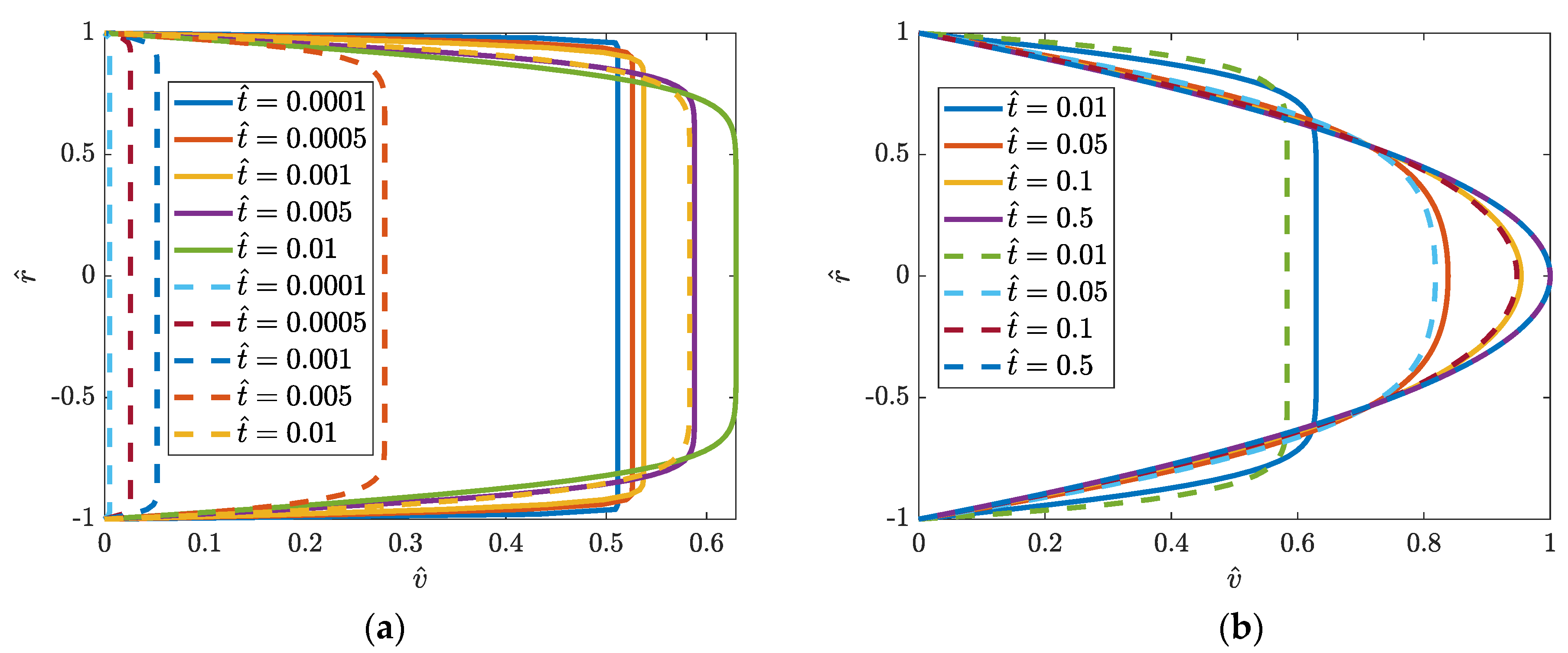
the Andersson and Tiseth solution is characterized by a non-physical jump in the flow rate from zero to 0.5. The above results from the fact that the velocity profile changes from a flat plug profile to a parabolic one over time (but maintains constant mean velocity). A similar change takes place at the entrance section from the reservoir to the pipe, as the parabolic profile is here formed along the pipe length in a similar way, which was noticed and described by Sparrow et al. [76];
-
the Das and Arrakeri model seems to be correct from a practical point of view; in this model, the velocity profile starts its development from the zero value (Figure 12);
-
the solution discussed in this section can be used in practice only in cases where the flow occurs as a result of the piston’s motion.

4. Accelerated Turbulent Pipe Flow—TULF Model by García García and Alvariño

In this section, the model that extends from steady to unsteady turbulent pipe flow will be discussed. The model is based on Pai’s [87] idea of decomposing the turbulent velocity profile to the sum of the Hagen–Poiseuille parabola and a purely turbulent component. The starting point of García García and Alvariño model (TULF model; TULF is an abbreviation for the theory of underlying laminar flow) is the non-homogeneous dimensionless Reynolds-averaged Navier–Stokes partial differential equation (RANSE) [84,88,89,90]:
v t ^ 2 v r ^ 2 + 1 r ^ v r ^ = p ^ x ^ 1 r ^ r ^ σ r ^ = Π t ^ + Σ t ^ , r ^
with the following initial and boundary conditions:
v 0 , r ^ = v 0 r ^ ,   v t ^ , 1 = 0 ,   v t ^ , 0 r ^ = 0
and knowledge of the dimensionless Reynolds-averaged continuity equation:
v x ^ = 0
In the above equations Π t ^ is the mean (minus) pressure gradient, σ t ^ , r ^ is the Reynolds Shear Stress (RSS) field, satisfying the condition σ t ^ , 0 = σ t ^ , 1 = 0 and the function Σ t ^ , r ^ = 1 r ^ r ^ σ r ^ is defined by the authors of this model as the Weighted Reynolds Shear Stress Gradient (WRSSG).
The new semi-analytical solution was obtained by García García and Alvariño [84,88,89,90] in the following steps:
(a)
solving the homogeneous equation (left-hand side of Equation (42)) for the boundary conditions (43). Firstly, it was split up into two ordinary differential equations (separate for variable r ^ and t ^ ). Equation with r ^ constitutes a classical Sturm–Liouville problem whose solution is the set of normalized eigenfunctions, while the other one (dependent on t ^ ) is a temporal equation. The final general transient velocity field solution takes a form similar to Fan’s solution obtained for impulsive pressure gradient (solution v ¯ 1 r ^ , t ^ mentioned under Equation (18)), the only differences were coefficients determined from initial conditions;
(b)
obtaining the solution for the non-homogeneous case with the help of an integrating factor and knowledge of the source functions Π t ^ and Σ t ^ , r ^ , which were assumed as well-behaved functions. The mean velocity field v t ^ , r ^ is composed of three terms: v I —corresponds to transient decay of the mean initial velocity v m , 0 ; v P —defines the unsteady response of the time-dependent mean pressure gradient; v R —source of velocity field caused by the turbulence’s Reynolds shear stress gradient. From [90], it follows that function Σ t ^ , r ^ can be treated as a sum of components of the eigenfunction expansions of σ / r ^ and σ / r ^ , respectively. In turbulent flows, the analytical form of σ t ^ , r ^ is not known, and must be determined from known reliable experimental data;
(c)
using Pai’s method [87], the mean velocity field v I can be composed as a sum of underlying laminar flow v I L t ^ , r ^ and the pure turbulent component v I T t ^ , r ^ . This allowed the decomposition of the general mean flow equation into the sum of two fields, laminar and turbulent, respectively (see block diagram in Figure 13), as proposed by García García and Alvariño. The temporal evolution of v L and v T are different, such a situation generates asynchronism (distortion) of the mean velocity field of unsteady flows resulting in many phenomena noticed earlier only in the experimental research. Many of them have been discussed and explained in the authors’ publications [84,89,90];
(d)
the mean pressure gradient (MPG) was assumed to undergo a linear change until reaching its final value. The MPG change time can be controlled directly by an experimenter (associated with the mean valve-aperture time), and therefore, it can be assumed that it will remain virtually unchanged in all realizations of the flow. The second source term, the RSS field, is strictly connected with turbulence. A linear homotopy transition of this field is assumed. It follows that RSS is modeled similarly to MPG, but the slope can be assumed differently ( Δ t ^ versus t ^ 2 will be discussed later on). Such a simplified ramp approach has one degree of freedom and singularities which can cause visible unrealistic peaks of final solutions, however, as shown in [84,90], the quality of the modeling compliance can be considered satisfactory. In starting flow from rest the RSS must evolve from a zero value to some constant value related to a steady-state final flow. To model the final state, the model of Pai is used [87], which gives acceptable results for moderate Reynolds numbers (it is a limitation of this semi-analytical model). The Pai model helps to define the initial and final flow in simple polynomial form.
Figure 13. TULF model component-wise block diagram of detailed velocity field decomposition.
Energies 16 01407 g013
The terms ( Π 0 , Π ; χ 0 , χ and q 0 , q ) that govern RSS, mean velocity and WRSSG are defined in [84] as Spatial Degrees of Freedom (SDoF) that need to be calculated for the initial and final times. They define the radial dependence of the relevant flow fields. Coefficient χ 0 is the initial centreline turbulent dissipation being the ratio v L t ^ = 0 , r ^ = 0 / v t ^ = 0 , r ^ = 0 of underlying laminar flow to the mean velocity at the centerline of the pipe. The turbulence field can be switched off if one assumes χ 0 = 1 . The other initial coefficient q 0 is a best-fitting integer power. The final values of the coefficients χ and q need to be defined from the experimental velocity profile of the final turbulent flow.
If the accelerated flow is started from rest then the initial values of RSS, velocity field and WRSSG are: σ 0 r ^ = 0 ; v 0 t ^ = 0 , r ^ = 0 and Σ 0 r ^ = 0 , while the final values can be calculated from the following equations [84]:
σ t ^ , r ^ Σ t ^ , r ^ = 0 2 η 2 3 2 η σ r ^ Σ r ^ σ r ^ Σ r ^ if   t ^ < t ^ 0 , if   t ^ 0 t ^ t ^ 2 , if   t ^ > t ^ 2 .
where η = t ^ t ^ 0 t ^ 2 t ^ 0 0 , 1 , t ^ 0 is the mean time of transition to turbulence; t ^ 2 is the mean turbulence-settling time. These times are not easily controlled by any experimenter (the values may change from one experiment to the other). They must be defined in the TULF model too, they are external parameters that cannot be determined from analytical theory. The relation between mentioned times t ^ 0 , t ^ 2 and Δ t ^ defined as Temporal Degrees of Freedom (TDoF) can be a source of division of the flows into four classes [84]:
(I)
t ^ 0 < Δ t ^ —here turbulence on average begins before the increase in MPG is over (early transition to turbulence);
(II)
t ^ 0 > Δ t ^ —the turbulence on average begins after the MPG becomes constant (late transition to turbulence);
(III)
t ^ 2 t ^ 0 < Δ t ^ —the turbulence’s increase rate is faster than that of MPG with an offset t ^ 0 (fast turbulence evolution);
(IV)
t ^ 2 t ^ 0 > Δ t ^ —the turbulence increases slower than the MPG, even after subtracting the offset (slow turbulence evolution).
The above four types of accelerated pipe flows are the subject of intensive research discussed in [84];
(e)
the use of formulas discussed in earlier points made it possible to determine the final solution for the terms v L t ^ , r ^ and v T t ^ , r ^ for the analyzed case of accelerated flow for appropriate ranges of dimensionless time.
The final solution [84] for v L t ^ , r ^ is:
(a)
for 0 t ^ Δ t ^ :
v L t ^ , r ^ = 12 Π t ^ Δ t ^ 3 n = 1 J 0 λ n r ^ λ n 9 J 1 λ n λ n 6 t ^ 3 3 + λ n 4 λ n 2 Δ t ^ 2 + 1 t ^ 2 + λ n 2 Δ t ^ + 2 1 λ n 2 t ^ e λ n 2 t ^
(b)
while for t ^ > Δ t ^ :
v L t ^ , r ^ = 12 Π t ^ Δ t ^ 3 n = 1 J 0 λ n r ^ λ n 9 J 1 λ n 2 λ n 2 Δ t ^ e λ n 2 t ^ Δ t ^ 2 + λ n 2 Δ t ^ e λ n 2 t ^ + λ n 6 Δ t ^ 3 6
And the final solution [84] for v T t ^ , r ^ :
(a)
for 0 t ^ t ^ 0 :
v T t ^ , r ^ = 0
(b)
for t ^ 0 < t ^ t ^ 2 :
v T ( t ^ , r ^ ) = Π ( t ^ ) t ^ 2 t ^ 0 2 q ( χ 1 ) χ ( q 1 ) n = 1 J 0 λ n r ^ λ n 6 J 1 λ n 2 1 F 2 q ; q + 1 , 1 ; λ n 2 4 2 J 1 λ n λ n 3 t ^ t ^ 0 λ n 2 1 2 + 1 2 e λ n 2 t ^ t ^ 0 2 t ^ 2 t ^ 0 λ n 2 t ^ t ^ 0 3 λ n 6 3 t ^ t ^ 0 2 λ n 4 + 6 t ^ t ^ 0 λ n 2 1 + e λ n 2 t ^ t ^ 0
(c)
for t ^ > t ^ 2 :
v T ( t ^ , r ^ ) = Π ( t ^ ) t ^ 2 t ^ 0 2 q ( χ 1 ) χ ( q 1 ) n = 1 J 0 λ n r ^ λ n 6 J 1 λ n 2 1 F 2 q ; q + 1 , 1 ; λ n 2 4 2 J 1 λ n λ n λ n 4 t ^ 2 t ^ 0 2 6 e λ n 2 t ^ t ^ 0 2 t ^ 2 t ^ 0 λ n 2 + 1 + 6 e λ n 2 t ^ t ^ 2 2 t ^ 2 t ^ 0 λ n 2 1
In Equations (49) and (50), F 1 2 a ; b , c ; x is the Generalized Hypergeometric function, which generally is calculated in the following way:
F 1 2 a ; b , c ; x = n = 1 a n b n c n x n n !
In Equation (51), z n is the Pochhammer’s symbol, which is defined as:
z n = z z + 1 z + 2 z + n 1 = k = 1 n z + k 1 = Γ z + n Γ z ,   z 0 = 1 ,   z
The complete accelerated solution is a sum of laminar and turbulent components:
v t ^ , r ^ = v L t ^ , r ^ + v T t ^ , r ^
An example of simulation with this model for a case of accelerated pipe flow from rest to R e = 56677 is presented in Figure 14. Input data for this early and slow class of accelerated flow are: Π t ^ = 4.0912 · 10 6 ; Δ t ^ = 0.006 ; q = 45 ; χ = 29.3758 ; t ^ 0 = 0.0042 ; t ^ 2 = 0.012 .
In summary, the TULF solution presented by García García and Alvariño is an interesting addition to the theory of analytical methods for solving this type of accelerated flow. With its help, it was possible to theoretically justify many phenomena occurring during accelerated flows (e.g., the hyperlaminar jet effect [91], the lone concavity [92], or the annular jet effect [40,85,93]), which until now had only been observed experimentally. These findings show the role of analytical solutions in the continuous scientific progress regarding the issues of transient liquid flows through pressurized pipes. They were derived assuming a pressure gradient change as a flow generator. This means that an equivalent solution could also be derived for forced flow by means of a piston.

5. Conclusions

Two types of accelerated flows described in the literature were analyzed: (1) acceleration as a result of a change in pressure gradient (occurs in systems where a change in pressure occurs as a result of a sudden opening of the gate valve) and (2) acceleration resulting from the assumption of a specific change in the flow rate (such a situation occurs in hydraulic systems with forced movement due to the displacement of piston elements). A survey of the literature shows that the standard 1932 Szymański’s solution has been independently derived much earlier by at least two scientists: (1) the Italian Roiti in 1871 and the Russian Gromeka in 1882, hence it should be quoted as the RGS solution, as adopted in this work from the letters of the authors’ surnames. An interesting solution, which is the prototype of the 1992 Andersson and Tiseth solution, was derived in 1933 by Vogelpohl. This combines the universal solution for any change in the pressure gradient discussed in detail in Section 2.3 of this work with solutions from the second group, i.e., flows forced by a jump in the flow rate. Vogelpohl succeeded in determining the pressure gradient function such that the average value of the flow velocity is kept constant (identical to that obtained almost sixty years later by Anderson and Tiseth). All the analytical solutions discussed in this work are of great practical value, as they give the opportunity to accurately analyze the variability in velocity profiles, mean velocity values (or pressure gradients), shear stresses on the pipe wall, dynamic friction coefficients, etc. Thanks to this, they are perfect for verifying commercial programs in the field of CFD (computational fluid dynamics). The completed review of known analytical models of accelerated flow indicates that Telionis was right when he wrote in his book that “impulsive fluid motions do not exist in reality”. In real life the motion of a piston is never instantaneous as assumed in the Anderson and Tiseth solution; similarly, an instantaneous pressure gradient never takes place in real systems (as an effect of the valve opening time). So real flow is always somewhere between these two solutions defined and discussed in this paper. In the case of accelerated flows resulting from the impact of the pressure gradient at the inlet and outlet of the conduit, it seems that further research is necessary to show the real time variability of pressure gradient functions in laminar flows. This will determine whether it can actually be described by a function similar to the one observed in experimental studies by Avula in 1968, if so, it will still be necessary to choose a function that will give a complete analytical solution (and not, as now, the integral of this function should be determined numerically). There is a need to summarize all scientific papers describing experimental studies of accelerated flows—most are focused on the transition between laminar and turbulent flow. Experimental studies strictly concerning only laminar flows (Re < 2320) are almost non-existent in the literature.
A drawback of the presented models is their mathematical complexity (infinite series). They are based on Bessel functions and their zeros. For these zeros no analytical formula has been developed to date, hence they must be determined numerically. Bessel functions, on which all discussed solutions of velocity profile are based, are still simulation problems, especially for very small and large arguments. To overcome this problem in the computer programs used to carry out sample comparisons presented in several figures, this function was expanded in a Taylor series for small arguments, and asymptotic formulas for large arguments were used. According to this approach, this solution should be approximated with much simpler functions to be more useful in practice.
A significant strength of the presented analytical solutions is the possibility to define other related flow parameter-time dependences: mean velocity (in pressure-gradient-driven flows), the pressure gradient (in flow-rate-driven flows), friction factor and wall shear stress. These parameters are very helpful for a better understanding of the accelerated flow characteristics.
The semi-analytical solution for turbulent flow (TULF model developed by García García and Alvariño) is the most complex of all the analyzed solutions. Here, the turbulent velocity field is dependent on Bessel functions, their zeros and a generalized hypergeometric function. There is no easy and straightforward way to define the required spatial degrees of freedom coefficients ( Π , χ and q —defining respectively: mean pressure gradient, initial centreline turbulent dissipation and best-fitting integer power). However, it is possible to theoretically investigate and better understand the behavior of experimentally discovered phenomena such as: the lone concavity, annular jet effect and hyperlaminar jet effect. This solution would be useful to study the behavior of other related phenomena not discovered experimentally yet. Finally, Table 2 summarizes the advantages and disadvantages of the reviewed analytical solutions.
In the present review, it was also noted that, to date, there is a lack of an analytical solution as well as experimental studies of the accelerated flow of Newtonian fluid in plastic conduits (HDPE, ABS, PVC, PP, PB). In these conduits, the water hammer theory implies that the additional damping is due to the delayed strains that occur during this type of flow. The influence of these deformations is taken into account in the equation of continuity and not momentum, so the question remains whether in accelerated flows the same profiles and development times will be obtained in pipes with identical parameters (diameter, roughness, wall thickness) but made of two different materials: plastic and metal.

Author Contributions

Conceptualization, K.U., A.B. and M.S.; methodology, K.U. and M.K.; software, K.U., M.K. and A.D.; validation, K.U., A.D. and M.S.; formal analysis, K.U., A.D. and M.S.; investigation, K.U., A.B, M.S. and M.K.; resources, K.U.; data curation, K.U. and A.D.; writing—original draft preparation, K.U. and A.B.; writing—review and editing, K.U., A.B., A.D. and M.S.; visualization, K.U. and M.K.; supervision, K.U. and A.B.; project administration, K.U. and M.S.; funding acquisition, K.U. and A.B. All authors have read and agreed to the published version of the manuscript.

Funding

A. Bergant gratefully acknowledges the support of the Slovenian Research Agency (ARRS) conducted through the research project L2-1825 and programme P2-0162.

Data Availability Statement

Codes generated during the study and experimental data are available from the corresponding author by request.

Conflicts of Interest

The authors declare no conflict of interest.

Nomenclature

Apipe cross-sectional area (m2)
aacceleration (m/s2)
b, kpositive constants in Smith solution
a1,…, a5calibrated constants of Avula’s pressure gradient field
c P specific heat capacity (J/(kgK))
Dpipe internal diameter (m)
ffriction factor (-)
Gnormalized pressure gradient (m/s2)
gacceleration due to gravity (m/s2)
g ˙ volumetric heat source term (W/ m 3 )
Hpressure head (m)
H ^ dimensionless head (-)
Lpipe length (m)
MOtis start-up parameter (-)
ppressure (Pa)
p dimensionless Avula’s pressure p = Δ p 2 ρ U 2 (-)
p ^ normalized pressure (-)
Q flow rate (m3/s)
Q normalized flow rate (-)
qbest fitting integer TULF model coefficient (-)
Rpipe internal radius (m)
Re Reynolds number Re = D v m ν (-)
rradial coordinate (m)
r ^ normalized radial coordinate (-)
sLaplace complex variable (s−1)
Ttemperature field (°C)
T 1 ,   ,   T 4 terms in Das-Arakeri solution
ttime (s)
t A dimensionless Avula’s time (-)
t ^ dimensionless time t ^ = t ν R 2 (-)
udummy variable in convolutions integrals (s)
vvelocity field (m/s)
vmmean velocity (m/s)
v ^ dimensionless velocity v ^ = v / v m a x (-)
v ˜ dimensionless García García and Alvariño velocity v ˜ = v · R / ν (-)
v dimensionless Avula’s velocity v = v / U (-)
v0initial velocity (m/s)
X dimensionless distance function (-)
xaxial coordinate (m)
x stretched axial coordinate (m)
x ^ normalized axial coordinate x ^ = x / R (-)
α thermal diffusivity coefficient (m2/s)
α n successive zeros of the Bessel function J 2 α n (-)
β 
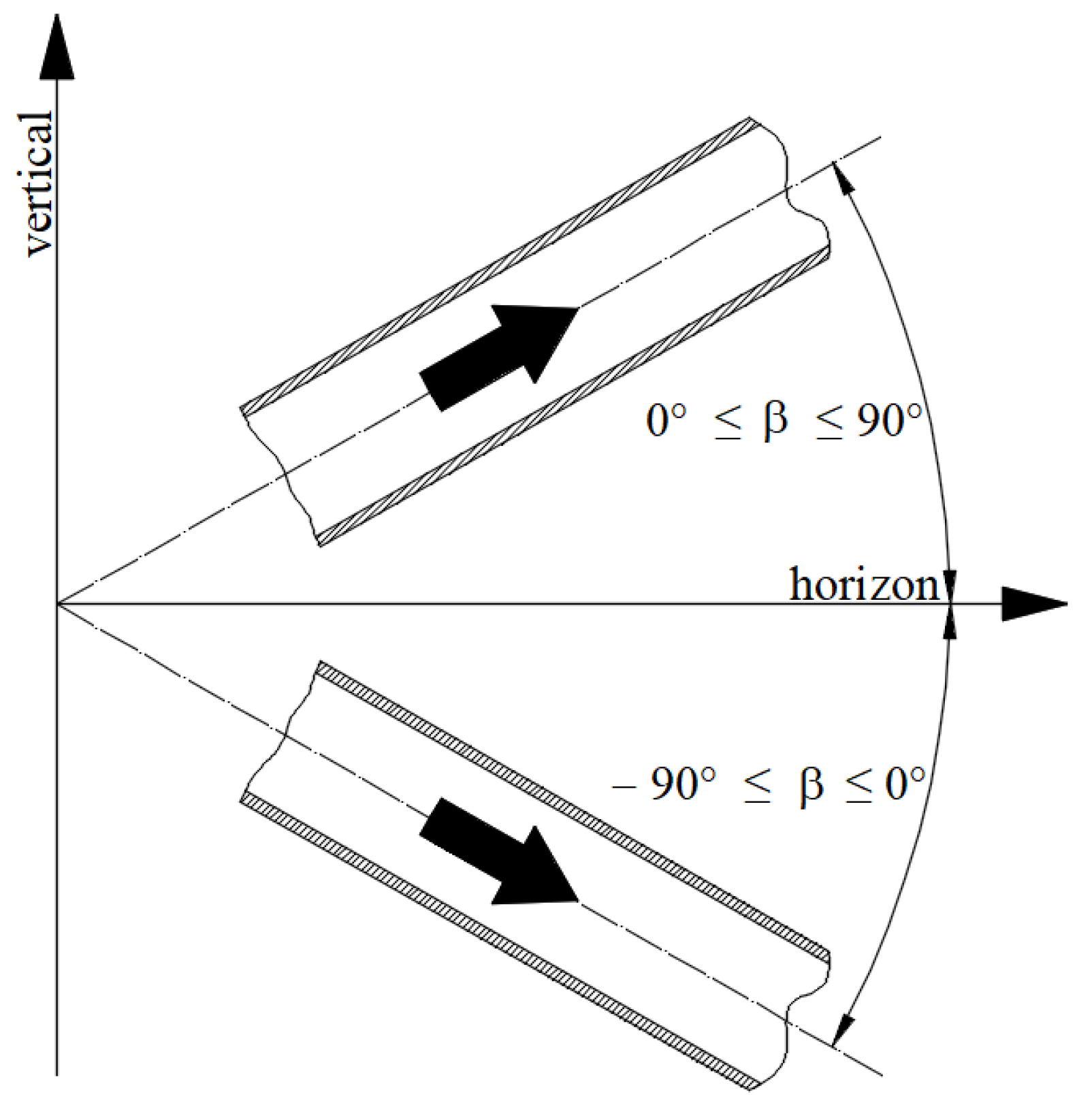
pipe slope angle (°)
γ specific weight of the liquid (N/m3)
Δ t ^ dimensionless time interval of linear MPG growth (mean valve aperture time) (-)
εjerk coefficient (m/s3)
η time scale coefficient in TULF model (-)
η n successive zeros of the Bessel function J 0 s R e / 2 (-)
λ n successive zeros of the Bessel function J 0 λ n (-)
μdynamic viscosity of liquid (Pa·s)
νkinematic viscosity of liquid (m2/s)
ξ n successive roots fulfilling relation J o R ξ n = 0 (m−1)
Π normalized mean pressure gradient in TULF solution (-)
ρdensity of liquid (kg/m3)
Σ weighted Reynolds shear stress gradient (-)
σ Reynolds shear stress field in TULF solution (-)
τwwall shear stress (Pa)
χ turbulent dissipation coefficient (-)
Subscripts
0 initial
m mean
o outlet
p piston
t transitional
i inlet
w wall
final
Acronyms
ATAnderson and Tiseth solution
DADas and Arakeri solution
IIto solution
KVNKannaiyan–Varathalingarajah–Natarajan solution
MPGmean pressure gradient
RANSEReynolds-averaged Navier–Stokes equation
RGSRoiti–Gromeka–Szymański solution
RGSIRoiti–Gromeka–Szymański-Ito solution
RSSReynolds shear stress
SSparrow solution
SMSmith solution
TULFtheory of underlying laminar flow
WRSSGweighted Reynolds shear stress gradient

References

  1. Navier, C.L.M.H. Mémoire sur les lois du mouvement des fluides. Mémoires L’académie R. Sci. L’institut Fr. 1823, 6, 389–440. [Google Scholar]
  2. Darrigol, O. Between Hydrodynamics and Elasticity Theory: The First Five Births of the Navier-Stokes Equation. Arch. Hist. Exact Sci. 2002, 56, 95–150. [Google Scholar] [CrossRef]
  3. Letelier S, M.F.; Leutheusser, H.J. Unified Approach to the Solution of Problems of Unsteady Laminar Flow in Long Pipes. J. Appl. Mech. 1983, 50, 8–12. [Google Scholar] [CrossRef]
  4. Urbanowicz, K.; Firkowski, M.; Bergant, A. Comparing analytical solutions for unsteady laminar pipe flow. In Proceedings of the 13th International Conference on Pressure Surges, Bordeaux, France, 14–16 November 2018; pp. 311–326. [Google Scholar]
  5. Roiti, A. Sul movimento dei liquidi. Ann. Della Sc. Norm. Super. Pisa—Cl. Sci. 1871, 1, 193–240. [Google Scholar]
  6. Betti, E. Alcune Determinazioni delle Temperature Variabili di un Cilindro. Tipografia dei FF; Nistri: Pisa, Italy, 1868. [Google Scholar]
  7. Gromeka, I.S. On a theory of the motion of fluids in narrow cylindrical tubes. Uch. Zap. Kazan. Inst. 1882, 112. (In Russian) [Google Scholar]
  8. Baibikov, B.S.; Oreshkin, F.; Prudovskii, A.M. Frictional resistance in the case of accelerated flow in a tube. Fluid Dyn. 1981, 16, 749–751. [Google Scholar] [CrossRef]
  9. Ovsyannikov, V.M. Calculation of accelerated motion of fluid in a tube. Fluid Dyn. 1981, 16, 770–772. [Google Scholar] [CrossRef]
  10. Logov, I.L. Frictional resistance to accelerated flow in a tube. Fluid Dyn. 1984, 18, 978–983. [Google Scholar] [CrossRef]
  11. Loitsyanskii, L.G. Mechanics of Liquids and Gases, 2nd revised ed.; International Series of Monographs in Aeronautics and Astronautics, Division II: Aerodynamics; Jones, R.T., Jones, W.P., Eds.; Pergamon Press: Oxford, UK, 1966; Volume 6, pp. 17–18. [Google Scholar]
  12. Gromeka, I.S. Collected Works; Izd. AN SSSR: Moscow, Russia, 1952. [Google Scholar]
  13. Szymański, P. Quelques solutions exactes des équations de l’hydrodynamique du fluide visqueux dans le cas d’un tube cylindrique. J. Math. Pures Appliquées 1932, 11, 67–108. [Google Scholar]
  14. Schlichting, H.; Gersten, K. Boundary Layer Theory, 9th ed.; McGraw-Hill: New York, NY, USA, 2017; p. 140. [Google Scholar]
  15. White, F.M. Viscous Fluid Flow, 3rd ed.; McGraw-Hill: New York, NY, USA, 2006; p. 125. [Google Scholar]
  16. Telionis, O.P. Unsteady Viscous Flows; Springer: New York, NY, USA, 1981; pp. 91–92. [Google Scholar]
  17. Gerbes, W. Zur instationären, laminaren Strömung einer inkompressiblen, zähen Flüssigkeit in kreiszylindrischen Rohren. Z. Angew. Phys. 1951, 3, 267–271. [Google Scholar]
  18. Ito, H. Theory of Laminar Flow through a Pipe with Non-Steady Pressure Gradients. Trans. Jpn. Soc. Mech. Eng. 1952, 18, 101–108. [Google Scholar] [CrossRef] [Green Version]
  19. Atabek, H.B. Development of flow in the inlet length of a circular tube starting from rest. ZAMP 1962, 13, 417–430. [Google Scholar] [CrossRef]
  20. Avula, X.J.R. Analysis of suddenly started laminar flow in the entrance region of a circular tube. Appl. Sci. Res. 1969, 21, 248–259. [Google Scholar] [CrossRef]
  21. Fan, C.; Chao, B.-T. Unsteady, laminar, incompressible flow through rectangular ducts. J. Appl. Math. Phys. (ZAMP) 1965, 16, 351–360. [Google Scholar] [CrossRef]
  22. Laura, P.A.A. Unsteady, laminar, incompressible flow through ducts of arbitrary, doubly connected cross section. Rev. De La Unión Matemática Argent. 1976, 27, 197–206. [Google Scholar]
  23. Muzychka, Y.; Yovanovich, M. Compact models for transient conduction or viscous transport in non-circular geometries with a uniform source. Int. J. Therm. Sci. 2006, 45, 1091–1102. [Google Scholar] [CrossRef]
  24. Muzychka, Y.; Yovanovich, M. Unsteady viscous flows and Stokes’s first problem. Int. J. Therm. Sci. 2010, 49, 820–828. [Google Scholar] [CrossRef] [Green Version]
  25. Chen, C.-I.; Yang, Y.-T. Unsteady unidirectional flow of an Oldroyd-B fluid in a circular duct with different given volume flow rate conditions. Heat Mass Transf. 2004, 40, 203–209. [Google Scholar] [CrossRef]
  26. Nazar, M.; Mahmood, A.; Athar, M.; Kamran, M. Analytic solutions for the unsteady longitudinal flow of an oldroyd-b fluid with fractional model. Chem. Eng. Commun. 2012, 199, 290–305. [Google Scholar] [CrossRef]
  27. Wang, X.; Xu, H.; Qi, H. Transient magnetohydrodynamic flow and heat transfer of fractional Oldroyd-B fluids in a microchannel with slip boundary condition. Phys. Fluids 2020, 32, 103104. [Google Scholar] [CrossRef]
  28. Rahaman, K.; Ramkissoon, H. Unsteady axial viscoelastic pipe flows. J. Non-Newtonian Fluid Mech. 1995, 57, 27–38. [Google Scholar] [CrossRef]
  29. Gerhart, P.M.; Gerhart, A.L.; Hochstein, J.I. Munson, Young, and Okiishi’s Fundamentals of Fluid Mechanics, 8th ed.; John Wiley and Sons: Hoboken, NJ, USA, 2016; p. 16. [Google Scholar]
  30. Vogelpohl, G. Über die Ermittlung der Rohreinlaufströmung aus den Navier-Stokesschen Gleichungen. ZAMM J. Appl. Math. Mech./Z. Angew. Math. Mech. Vorträge Hauptversamml. Würzburg Ges. Angew. Math. 1933, 13, 422–449. [Google Scholar] [CrossRef]
  31. Whittaker, E.T. On the numerical solution of integral-equations. Proc. R. Soc. London. Ser. A 1918, 94, 367–383. [Google Scholar] [CrossRef] [Green Version]
  32. Andersson, H.I.; Tiseth, K.L. Start-up flow in a pipe following the sudden imposition of a constant flow rate. Chem. Eng. Commun. 1992, 112, 121–133. [Google Scholar] [CrossRef]
  33. Weinbaum, S.; Parker, K.H. The laminar decay of suddenly blocked channel and pipe flows. J. Fluid Mech. 1975, 69, 729–752. [Google Scholar] [CrossRef]
  34. Andersson, H.; Kristoffersen, R. Start-up of laminar pipe flow. In Proceedings of the AIAA/ASME/SIAM/APS 1st National Fluid Dynamics Congress, Cincinnati, OH, USA, 25–28 July 1988; pp. 1356–3805. [Google Scholar] [CrossRef]
  35. Otis, D.R. Laminar Start-Up Flow in a Pipe. J. Appl. Mech. 1985, 52, 706–711. [Google Scholar] [CrossRef]
  36. DAS, D.; Arakeri, J.H. Transition of unsteady velocity profiles with reverse flow. J. Fluid Mech. 1998, 374, 251–283. [Google Scholar] [CrossRef] [Green Version]
  37. Kannaiyan, A.; Varathalingarajah, T.; Natarajan, S. Analytical solutions for the incompressible laminar pipe flow rapidly subjected to the arbitrary change in the flow rate. Phys. Fluids 2021, 33, 043601. [Google Scholar] [CrossRef]
  38. Van de Sande, E.; Belde, A.P.; Hamer, B.J.G.; Hiemstra, W. Velocity profiles in accelerating pipe flows starting from rest. In Proceedings of the 3rd International Conference on Pressure Surges, Canterbury, UK, 25–27 March 1980; pp. 1–14, paper A1. [Google Scholar]
  39. Lefebvre, P.J.; White, F.M. Experiments on Transition to Turbulence in a Constant-Acceleration Pipe Flow. J. Fluids Eng. 1989, 111, 428–432. [Google Scholar] [CrossRef]
  40. Kataoka, K.; Kawabata, T.; Miki, K. The start-up response of pipe flow to a step change in flow rate. J. Chem. Eng. Jpn. 1975, 8, 266–271. [Google Scholar] [CrossRef]
  41. Chaudhury, R.A.; Herrmann, M.; Frakes, D.H.; Adrian, R.J. Length and time for development of laminar flow in tubes following a step increase of volume flux. Exp. Fluids 2015, 56, 22. [Google Scholar] [CrossRef]
  42. He, K.; Seddighi, M.; He, S. DNS study of a pipe flow following a step increase in flow rate. Int. J. Heat Fluid Flow 2016, 57, 130–141. [Google Scholar] [CrossRef] [Green Version]
  43. Deville, M.O. An Introduction to the Mechanics of Incompressible Fluids; Springer: Cham, Switzerland, 2022; p. 20. [Google Scholar] [CrossRef]
  44. Poisson, S.D. Mémoire sur la distribution de la chaleur dans les corps solides. J. L’ecole Polytech. 1823, 19, 249–403. [Google Scholar]
  45. Allievi, L. Teoria generale del moto perturbato dell’acqua nei tubi in pressione (colpo d’ariete). Il Politec.—G. Dell’ingegnere Archit. Civ. Ed Ind. (Fasc.) 1903, 33, 360–371. [Google Scholar]
  46. Fassò, C.A. Avviamento del moto di una corrente liquida in un tubo disezione costante: Influenza delle resistenze. Reniconti Inst. Lomb.—Acad. Sci. E Lett. 1956, 90, 305–342. [Google Scholar]
  47. Aresti, G. Sul moto di un fluido viscoso, incompressible, lungo un tubu cylindrico (rotondo). Rend. Semin. Della Fac. Sci. dell’Università Cagliari 1934, 4, 91–93. [Google Scholar]
  48. Szymański, P. Sur l’écoulement non permanent du fluide visqueux dans le tuyau. In Proceedings of the III Congrès International de Mécanique Appliquée, Stockholm, Sweden, 24–29 August 1930; pp. 249–254. [Google Scholar]
  49. Urbanowicz, K.; Tijsseling, A.S.; Firkowski, M. Comparing convolution-integral models with analytical pipe- flow solutions. J. Phys. Conf. Ser. 2016, 760, 012036. [Google Scholar] [CrossRef]
  50. Letelier S, M.F.; Leutheusser, H.J. Skin Friction in Unsteady Laminar Pipe Flow. J. Hydraul. Div. 1976, 102, 41–56. [Google Scholar] [CrossRef]
  51. Lefèbvre, P.J.; White, F.M. Further Experiments on Transition to Turbulence in Constant-Acceleration Pipe Flow. J. Fluids Eng. 1991, 113, 223–227. [Google Scholar] [CrossRef]
  52. Knisely, C.W.; Nishihara, K.; Iguchi, M. Critical Reynolds Number in Constant-Acceleration Pipe Flow from an Initial Steady Laminar State. J. Fluids Eng. 2010, 132, 091202. [Google Scholar] [CrossRef]
  53. Avula, X.J.R. A Combined Method for Determining Velocity of Starting Flow in a Long Circular Tube. J. Phys. Soc. Jpn. 1969, 27, 497–502. [Google Scholar] [CrossRef]
  54. Avula, X.J.R.; Young, D.F. Start-up Flow in the Entrance Region of a Circular Tube. ZAMM-J. Appl. Math. Mech./Z. Angew. Math. Mech. 1971, 51, 517–526. [Google Scholar] [CrossRef]
  55. Smith, S.H. Classroom Note: Time-Dependent Poiseuille Flow. SIAM Rev. 1997, 39, 511–513. [Google Scholar] [CrossRef]
  56. Dryden, H.L.; Murnaghan, F.D.; Bateman, H. Hydrodynamics; Dover: New York, NY, USA, 1956. [Google Scholar]
  57. Singh, T. Incipient flow of elastico-viscous fluid in a pipe. Eng. Comput. 1992, 9, 81–91. [Google Scholar] [CrossRef]
  58. Patience, G.S.; Mehrotra, A.K. Discussion: “Laminar Start-Up Flow in a Pipe”. J. Appl. Mech. 1987, 54, 243–244. [Google Scholar] [CrossRef] [Green Version]
  59. Fargie, D.; Martin, B.W. Developing laminar flow in a pipe of circular cross-section. Proc. R. Soc. Lond. Ser. A 1971, 321, 461–476. [Google Scholar] [CrossRef]
  60. Patience, G.S.; Mehrotra, A.K. Laminar start-up flow in short pipe lengths. Can. J. Chem. Eng. 1989, 67, 883–888. [Google Scholar] [CrossRef]
  61. Fan, C. Non-Steady, Viscous, Incompressible Flow in Cylindrical and Rectangular Conduits (with Emphasis on Periodically Oscillating Flow). Ph.D Thesis, University of Illinois, Champaign, IL, USA, 1964. [Google Scholar]
  62. Daneshyar, H. Development of unsteady laminar flow of an incompressible fluid in a long circular pipe. Int. J. Mech. Sci. 1970, 12, 435–445. [Google Scholar] [CrossRef]
  63. Sneddon, I.N. Fourier Transforms; McGraw-Hill: New York, NY, USA, 1951. [Google Scholar]
  64. Roller, J.E. Unsteady Flow in a Smooth Pipe after Instantaneous Opening of a Downstream Valve. Master’s Thesis, Georgia Institute of Technology, Atlanta, GA, USA, 1956. [Google Scholar]
  65. Zielke, W. Frequency-Dependent Friction in Transient Pipe Flow. Ph.D. Thesis, University of Michigan, Ann Arbor, MI, USA, 1966. [Google Scholar]
  66. Hershey, D.; Song, G. Friction factors and pressure drop for sinusoidal laminar flow of water and blood in rigid tubes. AIChE J. 1967, 13, 491–496. [Google Scholar] [CrossRef]
  67. Xiu, W.; Sun, J.G.; Sha, W.T. Transient flows and pressure waves in pipes. J. Hydrodyn. Ser. B 1995, 2, 51–59. [Google Scholar]
  68. Sun, J.G.; Wang, X.Q. Pressure transient in liquid lines. In Proceedings of the ASME/JSME Pressure Vessels and Piping Conference, Honolulu, HI, USA, 23–27 July 1995. [Google Scholar]
  69. Lee, Y. Analytical solutions of channel and duct flows due to general pressure gradients. Appl. Math. Model. 2017, 43, 279–286. [Google Scholar] [CrossRef]
  70. Song, G. Determination of Friction Factors for the Pulsatile Laminar Flow of Water and Blood in Rigid Tubes. Ph.D. Thesis, University of Cincinnati, Cincinnati, OH, USA, 1966. [Google Scholar]
  71. Avula, X.J.R. Unsteady Flow in the Entrance Region of a Circular Tube. Ph.D. Thesis, Iowa State University, Ames, IA, USA, 1968. [Google Scholar]
  72. Erdogan, M.E. On the flows produced by sudden application of a constant pressure gradient or by impulsive motion of a boundary. Int. J. Non-Linear Mech. 2003, 38, 781–797. [Google Scholar] [CrossRef]
  73. Müller, W. Zum Problem der Anlaufströmung einer Flüssigkeit im geraden Rohr mit Kreisring- und Kreisquerschnitt. ZAMM-J. Appl. Math. Mech./Z. Angew. Math. Mech. 1936, 16, 227–238. [Google Scholar] [CrossRef]
  74. Avramenko, A.A.; Tyrinov, A.I.; Shevchuk, I.V. An analytical and numerical study on the start-up flow of slightly rarefied gases in a parallel-plate channel and a pipe. Phys. Fluids 2015, 27, 042001. [Google Scholar] [CrossRef]
  75. Kuznetsov, A.V.; Avramenko, A.A. Start-Up Flow in a Channel or Pipe Occupied by a Fluid-Saturated Porous Medium. J. Porous Media 2009, 12, 361–367. [Google Scholar] [CrossRef]
  76. Sparrow, E.M.; Lin, S.H.; Lundgren, T.S. Flow Development in the Hydrodynamic Entrance Region of Tubes and Ducts. Phys. Fluids 1964, 7, 338. [Google Scholar] [CrossRef]
  77. Vardy, A.E.; Brown, J.M. Influence of time-dependent viscosity on wall shear stresses in unsteady pipe flows. J. Hydraul. Res. 2010, 48, 225–237. [Google Scholar] [CrossRef]
  78. Vardy, A.E.; Brown, J.M.B. Laminar pipe flow with time-dependent viscosity. J. Hydroinform. 2011, 13, 729–740. [Google Scholar] [CrossRef] [Green Version]
  79. Daprà, I.; Scarpi, G. Unsteady Flow of Fluids with Arbitrarily Time-Dependent Rheological Behavior. J. Fluids Eng. 2017, 139, 051202. [Google Scholar] [CrossRef]
  80. Wiens, T.; Etminan, E. An Analytical Solution for Unsteady Laminar Flow in Tubes with a Tapered Wall Thickness. Fluids 2021, 6, 170. [Google Scholar] [CrossRef]
  81. Cengel, Y.A. Heat Transfer a Practical Approach, 2nd ed.; Mcgraw-Hill: New York, NY, USA, 2002; p. 70. [Google Scholar]
  82. Moss, E.A. Laminar pipe flows accelerated from rest. N&O J. 1991, 7–14. [Google Scholar]
  83. Pozzi, A.; Tognaccini, R. The effect of the Eckert number on impulsively started pipe flow. Eur. J. Mech. B Fluids 2012, 36, 120–127. [Google Scholar] [CrossRef]
  84. García, F.J.G.; Alvariño, P.F. On the influence of Reynolds shear stress upon the velocity patterns generated in turbulent starting pipe flow. Phys. Fluids 2020, 32, 105119. [Google Scholar] [CrossRef]
  85. Maruyama, T.; Kato, Y.; Mizushina, T. Transition to turbulence in starting pipe flows. J. Chem. Eng. Jpn. 1978, 11, 346–353. [Google Scholar] [CrossRef] [Green Version]
  86. Kannaiyan, A.; Natarajian, S.; Vinoth, B.R. Stability of a laminar pipe flow subjected to a step-like increase in the flow rate. Phys. Fluids 2022, 34, 06410. [Google Scholar] [CrossRef]
  87. Pai, S. On turbulent flow in circular pipe. J. Frankl. Inst. 1953, 256, 337–352. [Google Scholar] [CrossRef]
  88. García García, F.J. Transient Discharge of a Pressurised Incompressible Fluid through a Pipe and Analytical Solution for Unsteady Turbulent Pipe Flow. Ph.D. Thesis, Higher Polytechnic College—University of A Coruña, A Coruña, Spain, 2017. Available online: https://hdl.handle.net/2183/18502 (accessed on 30 November 2022).
  89. García, F.J.G.; Alvariño, P.F. On an analytic solution for general unsteady/transient turbulent pipe flow and starting turbulent flow. Eur. J. Mech. B Fluids 2018, 74, 200–210. [Google Scholar] [CrossRef]
  90. García, F.J.G.; Alvariño, P.F. On an analytical explanation of the phenomena observed in accelerated turbulent pipe flow. J. Fluid Mech. 2019, 881, 420–461. [Google Scholar] [CrossRef]
  91. Annus, I.; Koppel, T.; Sarv, L.; Ainola, L. Development of Accelerating Pipe Flow Starting from Rest. J. Fluids Eng. 2013, 135, 111204. [Google Scholar] [CrossRef]
  92. Kurokawa, J.; Morikawa, M. Accelerated and Decelerated Flows in a Circular Pipe: 1st Report, Velocity Profile and Friction Coefficient. Bull. JSME 1986, 29, 758–765. [Google Scholar] [CrossRef]
  93. Viola, J.P.; Leutheusser, H.J. Experiments on Unsteady Turbulent Pipe Flow. J. Eng. Mech. 2004, 130, 240–244. [Google Scholar] [CrossRef]
Figure 1. Layout of the pipe considered in the present review.
Energies 16 01407 g001
Figure 2. Changes of pressure gradients: (a) step change from rest, (b) step change from initial to final value, (c) linear increase (d) ramp change.
Energies 16 01407 g002
Figure 3. Development of velocity profile in RGS-accelerated flow driven by a step change of pressure gradient.
Energies 16 01407 g003
Figure 4. Definition of pipe slope angle (adapted from [49]).
Energies 16 01407 g004
Figure 5. Exemplary variation of pressure gradient with time R e 1600 .
Energies 16 01407 g005
Figure 6. Velocity profiles comparison of RGS and Avula solutions for relatively: (a) small times; (b) large times (adapted from [53]).
Energies 16 01407 g006
Figure 7. Time variation of discharge.
Energies 16 01407 g007
Figure 8. Otis reference drawing indicating time variation of energy grade line (adapted from [35]).
Energies 16 01407 g008
Figure 9. Development of velocity profile in AT accelerated flow driven by an abruptly imposed constant volume flux.
Energies 16 01407 g009
Figure 10. Normalized axial velocity comparison of RGS and AT solutions.
Energies 16 01407 g010
Figure 11. Typical trapezoidal variation of piston velocity (motion) with time.
Energies 16 01407 g011
Figure 12. Comparison of Das and Arakeri model (dotted lines; t 0 ^ = 0.01 ) with Anderson and Tiseth model (solid lines): (a) t ^ 0.01 , (b) t ^ 0.01 .
Energies 16 01407 g012
Figure 14. Results of calculation using the García García and Alvariño TULF model: (a) early stage; (b) late stage.
Energies 16 01407 g014
Table 1. A list of works in which a universal formula was derived.
NoAuthor/sYearReference
1Vogelpohl1933[30]
2Roller1956[64]
3Fan1964[61]
4Song1966, 1967[66,70]
5Zielke1966[65]
6Avula1968, 1969[53,71]
7Daneshyar1970[62]
8Xiu et al.1995[67]
9Sun and Wang1995[68]
10Lee2017[69]
Table 2. Short summary of the reviewed analytical solutions valid for laminar accelerating pipe flow (except TULF model).
Imposed Pressure Gradient
SolutionEquation/sAdvantagesDisadvantages
RGSI
[5,7,13,18]
(9)able to calculate the unsteady velocity
profile for instantaneous pressure
gradient changes (not necessary from rest)
in original form valid only for horizontal infinite long pipes—Urbanowicz’s correction needed for sloping pipe
I
[18]
(11)showed what would be the mathematical solution of first stage of ramp change of the pressure gradientuselessness in practise, as the pressure gradient should stabilize as in unsolved case of ramp change
Avula
[53]
(13)promising results that more faithfully illustrate the real history of the velocity-profile changes in real systemscomplicated normalization (Re number dependence) used by Avula, which ended up with complicated zeros of the Bessel function. Not fully analytically solvable, as a result of the applied approximation form of the pressure gradient
general
[30,61,62]
(26)useful for general mathematical form of pressure gradient (suggested assumptions of pressure gradients that will give analytical solution of this integral)convolution integral of pressure gradient and exponential function need to be solved (analytically—suggested, or numerically)
TULF
[84,88,89,90]
(46)–(50)only one developed for turbulent flow, theoretically possible investigation of experimentally discovered phenomena (the lone concavity, annular jet effect, hyperlaminar jet effect)no easy and straightforward way to define the required spatial degrees of freedom coefficients, use of generalized hypergeometric function needed
Imposed Flow Rate
AT
[32]
(31)valid for finite-length tubes at locations beyond the entrance flow development lengthassumes unphysical jump (change) of axial velocity from 0 to 0.5 value
DA
[36]
(35) and (36)based on a more realistic ramp change of flow rate assumption (unphysical velocity jump excluded)—the results are more consistent with experiments in early stage of accelerationtwo different solutions defined for piston acceleration and constant piston velocity. Unclear rule to select time t0 defining finish of the piston acceleration period
KVN
[37]
(40)generalized AT and DA solutions, gives the possibility to derive the solution for acceleration from one steady state (or developing one) to other steady flow (a condition of double-step changes of the flow rate introduced)non-linear increase phase assumed, which gives unrealistic jump of the axial velocity in calculations
Disclaimer/Publisher’s Note: The statements, opinions and data contained in all publications are solely those of the individual author(s) and contributor(s) and not of MDPI and/or the editor(s). MDPI and/or the editor(s) disclaim responsibility for any injury to people or property resulting from any ideas, methods, instructions or products referred to in the content.

