Abstract
In January 2019, the Canadian province of Alberta enacted limits on crude oil and bitumen production. These production controls, a policy referred to as curtailment, represent a shift for a government that historically avoided market intervention. The policy was designed to shrink a growing and prolonged price differential between the Western Canadian Select price of oil, the key benchmark for Alberta’s heavy oil production, and the West Texas Intermediate benchmark. The curtailment created artificial scarcity, shrinking the price differential from more than $40 USD per barrel in November 2018 to less than $15 USD per barrel in February 2019. In the process, this policy transferred market surplus from refiners, mainly those in the US Midwest, to producers in Alberta. We review this large-scale market intervention and calculate the magnitude of the economic transfer. We find the curtailment increased producer surplus by $659M CAD per month and reduced consumer surplus by $763M per month. At the margin, every $1 reduction in consumer surplus translates into a $0.71 gain in producer surplus. We further show that if the Government of Alberta’s objective was to maximize short-run producer surplus, it should further scale back production, setting the curtailment rate at 25% rather than the initial 8.7%.
JEL Classification:
Q48; L71; L52
1. Introduction
In December 2018, the Canadian province of Alberta announced controls on crude oil and bitumen production, effective January 2019. The primary outcome of these production controls, a policy known as curtailment, involved transferring market surplus from refiners, mainly those in the US Midwest, to producers in Alberta. Traditionally, governments in Canada and the US have been reluctant to intervene in the day-to-day operations of oil markets. The curtailment, therefore, represents a notable interventionist shift in the production and marketing of crude oil and bitumen. (Canada ended interventionist policy in oil and natural gas markets in the late 1980s [1,2,3].) This situation presents a unique opportunity to examine an intervention in crude oil markets by a non-OPEC state. Specifically, we answer the question how is market surplus redistributed between producers and refiners as a result of Alberta’s production curtailment policy? We do this by measuring the magnitude of surplus transfer via estimating short-run demand and supply elasticities.
Our focus is the distribution of surplus after the government intervention rather than the causal effect of the intervention on prices. Yet, the impetus for Alberta’s intervention was the growing and prolonged price differential between the Western Canadian Select (WCS) price of oil price, the key benchmark for Alberta’s heavy oil production, and the West Texas Intermediate (WTI) benchmark. The WCS blend is a heavy oil with higher sulfur content (sour), a product that typically sells at a discount to the lighter, sweeter WTI. (WCS is a heavy (API density 20.5–21.5°), sour (3.0–3.5%) blend of bitumen, heavy and conventional oils produced in Western Canada. The benchmark is priced in Hardisty, Alberta, and managed as a daily volume-weighted index by Argus, based on production from Canadian Natural Resources, Cenovus Energy, Suncor Energy, and Talisman Energy. Because bitumen and heavy oils are blended with condensate or diluent, WCS is classified as a dilbit, or diluted bitumen.) Figure 1 illustrates that beginning in August 2018, the WCS diverged from the WTI, with the price differential between the benchmarks increasing from an average of $12.77/barrel (bbl) in 2017 to more than $45/bbl [4]. Moreover, two light-sweet oil benchmarks in Alberta—Edmonton Light Sweet and Syncrude Synthetic Sweet—whose prices normally track WTI fairly closely also diverged sharply in August 2018. The cause of the increase in the price differential was threefold: an increase in Western Canadian production while domestic demand and pipeline export capacity remained constant, combined with US refinery maintenance decreasing import demand [5]. Total Western Canadian production in September 2018 was 4.3 million barrels per day, and pipeline capacity was 3.95 million barrels per day [5]. The sudden, persistent and large difference in prices prompted industry leaders to express concerns about the financial health and economic viability of the sector, not to mention the attendant ramifications for the province’s budget [6]. The differential also ignited calls for a policy response. As owner of the resource, the Government of Alberta earns royalties on revenues from oil production, revenues that support the province’s operating budget [7]. Lower domestic prices entail lower revenues from oil production and hence lower royalty payments, as well as a lower willingness to pay by firms for future production rights. As a consequence, the Government of Alberta intervened in the market, limiting the quantity of crude oil and bitumen that the province’s 25 largest firms were permitted to produce and, accordingly, increased the price of oil exiting the province.
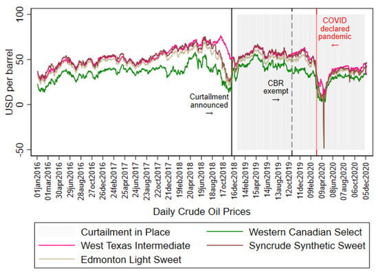
Figure 1.
Daily Crude Oil Prices, 2016–2020 [8,9]. Western Canadian Select (WCS) is a key benchmark for Alberta heavy oil production, Edmonton Light Sweet is a benchmark for Alberta light oil production, and Syncrude Synthetic Sweet is a benchmark for Alberta synthetic crude oil (derived from the oil sands). “CBR” is crude by rail, which became exempt from curtailment on 28 October 2019. See Figure 2 for the full timeline.
We study Alberta’s curtailment policy, in place from 1 January 2019 to 30 November 2020. Producers in the province represent one side of the market, and interventions that support suppliers come at a cost to demanders. By restricting supply and increasing the price, the curtailment transferred surplus from the consumers (refiners) of Alberta’s crude oil and bitumen to producers in Alberta, including the government as the owner of the resource. Transfers are not costless, however. The government’s intervention created an artificial scarcity and deadweight loss. The contribution of the paper involves measuring the magnitude of the surplus transfer and ensuing deadweight loss. We do this both at the margin, our preferred statistics (i.e., we measure the deadweight loss of the last dollar transferred), and in aggregate. We find the transfer to be large. Our preferred results imply a monthly increase in producer surplus on the order of $659 M, with each additional $1 dollar transferred generating a marginal deadweight loss of $0.29. The total deadweight loss for the market is estimated to be $104 M. That is, demanders of Albertan oil forfeited $763 M per month to facilitate the increase in WCS prices and improved producer margins.
Notwithstanding the market-level inefficiencies, we also show that the curtailment rate instituted by Alberta, a rate initially set at 8.7%, is actually smaller than the industry-wide profit-maximizing rate. If the Government of Alberta wanted to maximize the joint profits of producers (i.e., operate as a cartel in oil production), we calculate that it should have curtailed production by 25%, an additional 16.3% over and above the initial 8.7%. Curtailing production by 25% would yield a monthly increase in producer surplus on the order of $1144 M, nearly half a billion dollars more per month than the existing policy. These results, of course, reflect the short-run implications of what was intended to be a temporary policy. This intervention, however, may have lingering echoes in the market, implications that we review in our discussion.
This paper fits within a growing literature studying the industrial organization of North American oil markets, which emphasizes how infrastructure bottlenecks enable firms to exploit shifting markets and capture rents. For example, Borenstein and Kellogg [12] evaluate joint refinery and transportation capacity constraints in the US Midwest. A new supply of light sweet crude from North Dakota, combined with pipeline capacity constraints in Cushing, Oklahoma (the terminal point for several pipelines and the delivery point for WTI), lowered refinery feed-stock costs in the Midwest. Borenstein and Kellogg found that virtually none of these lower costs were passed through to gasoline or diesel prices, suggesting refiners obtained rents from the cost shock. McRae [13] likewise studies ConocoPhillips’ ownership of the Seaway pipeline connecting Cushing to Texas. Despite the build-up in supply in Oklahoma and an increasing differential between the WTI and Louisiana Light Sweet benchmarks, ConocoPhillips appears to have strategically delayed the pipeline’s reversal, enabling its refineries to obtain lower-cost feedstock. McRae calculates that ConocoPhillips’ refineries in the Midwest earned an additional $2 million per day. Walls and Zheng [14] examine how the post-2011 US oil production increase due to the shale boom affects refiners’ profitability, finding a 1% drop in WTI increases independent refiners’ operating incomes by 3%. Muehlegger and Sweeney [15] study how refinery market power influences cost pass-through in the US, finding that pass-through rates increase from effectively zero at the firm level to approximately 45% at the national scale. Specific to Alberta, Walls and Zheng [16] and Galay and Thille [17] examine the effect of pipeline capacity constraints on price differentials. Walls and Zheng quantify the magnitude of the transfer from producers to refiners and refined-product consumers within Western Canada, a small effect compared to the losses of upstream producers. Galay and Thille find takeaway capacity is constrained 38% of the time. Each of these papers, like the present one, explores the distribution of market surplus by studying the details of a specific characteristic of North American oil markets. Each of them also demonstrates the large swings in producer and consumer surplus that arise from these features. Our paper is unique, however, in that we examine the effect of policy intervention on surplus transfer rather than independent market forces or firms’ strategic behavior. Closest to our work is Hallak et al. [18], who examine how firms responded to the production quota and found producers shut in wells and reduced drilling. We abstract from firm behavior and identify the effect of these changes on market surplus.
We proceed as follows. Section 2 reviews pertinent details of the curtailment policy. Section 3 presents the economics of the transfer, including our conceptual framework and sketches of the formulae used to determine the magnitudes of Alberta’s intervention (Section 3.1); econometric methods (Section 3.2); and how we obtain the elasticities needed to calculate the implications of the intervention (Section 3.3). We estimate Alberta-specific elasticities but are guided by consensus estimates from the literature. We present results in Section 4, with sensitivity analysis and our estimate of an optimal curtailment rate. We discuss the longer-term implications of the curtailment in Section 5. Section 6 concludes.
2. Background on the Curtailment
The curtailment was announced in October 2018, and remained in place between January 2019 and December 2020. Figure 2 presents a timeline of notable decisions. The curtailment was motivated by the widening price differential between oil prices. Three factors led to the increased gap between Western Canadian prices and the WTI during late 2018 and, eventually, to Alberta’s intervention in the oil market. First, over the past decade, heavy oil and bitumen operators dramatically increased output. In 2018, Western Canadian production of heavy crude and bitumen averaged 2.3 million barrels per day (bpd) with total oil production of 4.4 million bpd [19]. Ten years earlier, in 2008, the total average monthly oil production was 2.4 million bpd with 1.0 million coming from heavy oil and bitumen [19]. Heavy oil and bitumen production increased by 130% within a decade. Bitumen production is either processed into a heavy crude oil that requires dilution to flow by pipeline, or further upgraded into a light, sweet synthetic crude oil. The distinction between “raw” and upgraded bitumen involves a process that is unique to oil sands and heavy oil production, largely in Alberta and Venezuela. At risk of oversimplifying, there are two types of refineries: simple refineries and high-conversion refineries. High-conversation refineries are able to handle heavy oil and raw bitumen without requiring prior processing; simple refineries cannot. For simple refineries to process bitumen, it must first be “upgraded” (processed) in an upgrading facility. Upgrading is a process whereby bitumen and heavy crude oil are partially cracked and chemically treated before their sale to downstream refineries. Upgrading yields a product known as synthetic crude oil. Further, to ship bitumen via pipeline, the oil must be diluted by blending it with condensate (e.g., naphtha), yielding a product normally referred to as dilbit (diluted bitumen); diluted by blending with synthetic crude oil, yielding synbit; or upgraded, yielding synthetic crude. Roughly one-third of Alberta’s heavy oil and bitumen is upgraded.
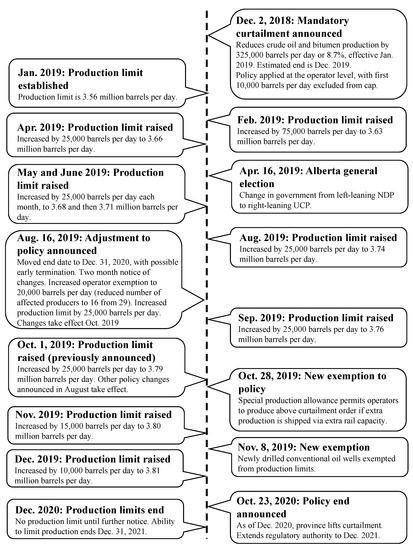
Figure 2.
Curtailment Timeline. Clancy [10] reports 28 firms affected by curtailment in January 2019, but a subsequent government announcement in August 2019 states 29 firms were affected [11].
The increase in production coincided with the second cause of the price differential. Infrastructure bottlenecks began to materialize in 2016, but became a regular feature of the market in late 2018. Given the increased production volumes, insufficient pipeline capacity existed to move products to markets. Pipeline bottlenecks also caused surplus storage capacity to rapidly dwindle. With insufficient pipeline capacity and limited storage options, Figure 3 shows how shippers were increasingly forced to ship barrels via rail and even by truck. Many, as a consequence, accepted low prices as they had fewer or more costly alternatives to place their physical product. These capacity constraints affected Western Canadian light oil prices in addition to heavy oil prices, as shown in Figure 1 and via price differentials as illustrated in Figure 4.
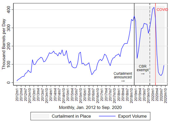
Figure 3.
Monthly Crude by Rail (CBR) Exports to the United States, 2012–2020 [20]. Excludes condensate. CBR became exempt from curtailment on 28 October 2019; see Figure 2 for full timeline.
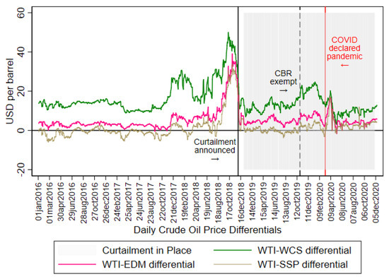
Figure 4.
Daily Oil Price Differentials, 2016–2020 [8,9]. Western Canadian Select (WCS) is a key benchmark for Alberta heavy oil production, Edmonton Light Sweet (EDM) is a benchmark for Alberta light oil production, and Syncrude Synthetic Sweet (SSP) is a benchmark for Alberta synthetic crude oil (derived from the oil sands). “CBR” is crude by rail, which became exempt from curtailment on 28 October 2019. See Figure 2 for full timeline.
The final reason for the late 2018 price differential comes from the consumer side of the market. Several refinery outages temporarily reduced the demand for Alberta’s heavy oil. These included both planned and unplanned maintenance at large refineries in Ohio, Wisconsin, Indiana, and Illinois [21,22].
In November 2018, Alberta’s oil production (excluding condensate) was 3.63 million barrels per day (peak production for the province), and in December 2018, it was 3.59 bpd. Alberta’s curtailment was announced on 2 December 2018 and commenced in January 2019 with Regulation 214/2018 [23]; see Figure 2 for the full timeline of the policy. The Government of Alberta identified production exceeded capacity by 190,000 bpd, and planned to cut production by 325,000 bpd, or 8.7% [24]. The new regulation granted Alberta’s Minister of Energy authority to establish a maximum combined production level for crude oil and bitumen in the province and the right to allocate production to specific operators. Production of lease condensate, a light hydrocarbon similar to very light crude oil, was exempt from curtailment. Operators with daily production at or above 10,000 barrels were affected, meaning 28 large firms were subject to the regulation [10]. (Clancy [10] reports 28 firms affected by curtailment in January 2019, but a subsequent government announcement in August 2019 states 29 firms were affected [11]. We hypothesize that between January and August, an additional firm’s production increased above the 10,000 barrel per day exemption, making it subject to curtailment.) Production from oil sands facilities and conventional production were regulated. Initially designed to terminate on 31 December 2019, the rules remained in place until December 2020. Further, if needed, the Government of Alberta stated that it reserved the right to re-introduce curtailment in 2021. In October 2020, it officially announced curtailment would end [25]. Figure 5 shows the curtailment cap started at 3.56 million bpd, and increased over 2019 and 2020 to end at 3.81 million bpd in November 2020. For the duration of the curtailment policy, actual production remained below the curtailment cap as depicted in Figure 5.
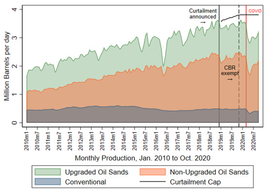
Figure 5.
Monthly Crude Oil Production, 2010–2020 [26]. Monthly crude oil production from conventional wells, oil sands, and upgraded oil sands. Excludes condensate. “CBR” is crude by rail, which became exempt from curtailment on 28 October 2019. See Figure 2 for the full curtailment timeline. The large dip in production in March 2016 is the Fort McMurray fire, and the dip in March 2017 is the explosion at the Syncrude oil sands facility.
The combination of increased supply, restricted transportation, and storage capacity, and lower demand generated the low late-2018 WCS prices seen in Figure 1. Figure 4 shows that prices in Alberta continued to diverge from the WTI benchmark. This generated increasing pressure on the government to intervene in the market, ultimately leading to the curtailment.
Alberta’s curtailment policy mimics a textbook production control policy. Quantity supplied is withheld from the market to increase prices received by producers. During the initial month of curtailment, as stated, aggregate provincial production was reduced by 325,000 bpd, equivalent to 8.7% of October 2018 production. Throughout most of 2019, the Government of Alberta slowly lessened the curtailment cap. The months of February through June saw curtailed volumes corresponding to 250,000, 250,000, 225,000, 200,000, and 175,000 bpd. Operator-specific allocations were determined via a formula based on an “adjusted baseline”, a value representing the best six months of production over the past year. The first baseline period began in November 2017 and terminated at the end of October 2018. Curtailment exemptions were provided for new entrants, and the rules did not apply to operators producing fewer than 10,000 bpd; the threshold was adjusted to 20,000 bpd in December 2019. This threshold implied that the policy only applied to a small handful (initially 28 out of 421) of operators in the province. Crude shipped by rail rather than via pipeline was also exempted from the curtailment starting in October 2019, while newly drilled conventional wells were exempted as of late November 2019.
Our analysis concentrates on the immediate short-run implications of the curtailment of producer and consumer (refiner) surplus. We seek to understand the magnitude of the transfer and its cost measured as the deadweight loss per dollar transferred on the margin. Independent of these values, however, we emphasize that there was a large and immediate market response to the Government of Alberta’s announcement. First, the WTI-WCS price differential, which averaged around $40/bbl (USD) for most of October and November 2018, plummeted to less than $15/bbl in mid-December 2018 and dropped below $10/bbl in January and February 2019. (The average differential between January 2013 and December 2020 is $17 USD per barrel.) Second, crude-by-rail shipments fell alongside the differential (Figure 3). Over 360,000 bpd were shipped by rail in December 2018, while only 130,000 bpd were moved via tanker cars in February 2019. To this end, the curtailment achieved its stated objective of reducing the WTI-WCS price differential. The gap between the WCS and WTI benchmarks dropped below its historical average within a month of the start of the policy.
The curtailment received mixed support from Alberta’s major oil producers, largely due to the policy’s differential effects on suppliers and consumers of Alberta’s heavy oil. Pure play producers such as Cenovus and Canadian Natural Resources, for example, expressed strong support for the government’s intervention [27]. These firms operate primarily on the production-side of the market, extracting oil and shipping it to other firms’ refineries. Consequently, they have few physical mechanisms to hedge low WCS prices. In contrast, several vertically integrated companies, firms engaged in both oil production and refining, did not support the curtailment (e.g., Imperial [28]). Low WCS prices enabled refineries owned by Suncor and Imperial Oil, for example, to obtain feedstock at lower costs while output prices remained constant. (Suncor, Imperial, and Husky Energy all own refineries and operate in the Alberta oil sands. Each of these firms’ production is markedly greater than their refinery capacity, however. Thus, intra-market effects, where, for instance, the vertically integrated firms attempt to lower rivals’ revenues by behaving strategically with respect to the pure play producers, are believed to be small. Notwithstanding this belief, we cannot eliminate strategic behavior as a contributor to the differential.) Lower production margins were offset by larger refining margins. Vertical integration acted as a hedge against the differential. Therefore, while our results concentrate on the distribution of surplus between Alberta’s oil producers and demanders of that oil, there are also cross-sectional distributional effects between the firms operating on the supplier side of the market. We return to these issues in Section 5.
Ultimately, the curtailment transferred surplus from consumers to producers, and a partial equilibrium model is useful to illustrate and quantify this transfer; we turn to this next.
3. Methods: Economics of Surplus Transfer
3.1. Conceptual Framework
Alberta’s curtailment policy was designed to reduce the WCS-WTI price differential and, in turn, transfer surplus from refiners of crude oil to producers. It accomplished this by limiting the quantity supplied, creating artificial scarcity, and leading to an increase in the price of Alberta’s heavy oil and bitumen. We use a partial equilibrium framework, as set out in Gardner [29], to quantify the economic magnitude of the surplus transfer, both in total and at the margin, demonstrating how these values depend on supply and demand elasticities.
We illustrate the intuition for the transfer in Figure 6. Figure 6 shows a blue demand curve and red supply schedule for Albertan oil (for the purpose of this exercise, we abstract from quality differences in the different types of Albertan oil and focus on heavy oil). Prior to production curtailment, the market price and quantity are given by and . Price, p, can be thought of as the WCS and Q as heavy oil and bitumen. The curtailment policy is a production control that limits output to , with higher prices paid by consumers as the consequence: increases to .
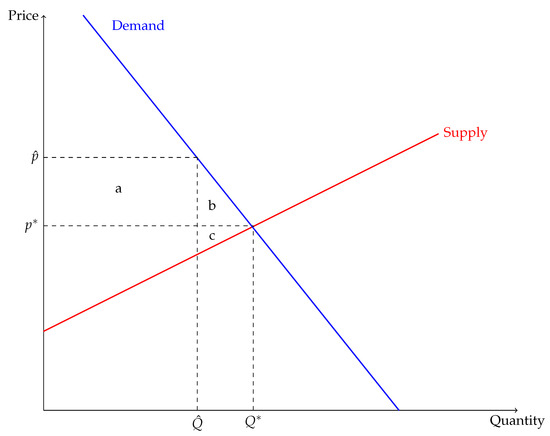
Figure 6.
The Effect of the Curtailment on Prices in Alberta’s Oil Market. Area a is the transfer from consumers (refiners) to producers; area b is lost consumer surplus; area c is lost producer surplus.
Two effects are apparent in Figure 6. First, the objective of the policy was to increase the price received by producers, thereby transferring surplus from consumers to producers. At , producers receive an additional per barrel relative to the pre-curtailment equilibrium. This is shown along the vertical axis. Region a illustrates the total value of the resulting transfer from consumers (refineries) to producers. It equals the increase in price, multiplied by the restricted output, . In order to obtain area a, however, producers forego region c, the producer surplus on the restricted supply, . If the size of a is greater than the size of c, as it is in Figure 6, Albertan oil producers are better off. Refiners, in turn, as demanders of crude bitumen, must pay a higher price for their feedstock and are unambiguously worse off.
A second implication of Figure 6 is that the production restrictions distort the market, creating deadweight loss. The deadweight loss, represented by area , arises because a smaller quantity of heavy oil and bitumen are supplied than would be the case without curtailment. This deadweight loss only arises if the equilibrium is given by and . A prospective argument, one argued by selected industry participants, is that pipeline bottlenecks distorted this equilibrium, and an alternative, inefficient equilibrium would have been obtained in the absence of the curtailment. Our opinion is that this is not the correct way to view this problem. Pipelines are not the only means of transportation. Rail and trucks are also used to ship crude and bitumen. Granted, they have higher costs and may be uneconomic (i.e., marginal costs increase with production), but they were viable modes of transport. Further, oil is storable, so placing barrels in storage is another option. A vital role of markets is to send signals to producers and consumers with respect to various demand and supply options. Prior to the curtailment, government intervention did not distort the market signals. Therefore, and is the appropriate “no policy” counterfactual. At the market level, then, a trade-off exists. Increases in producer surplus are offset by increases in overall deadweight loss. We measure this trade-off, both in absolute value and at the margin, as the deadweight loss per marginal dollar transferred.
Figure 6, finally, demonstrates how the government’s curtailment decision is akin to a monopolist’s problem (i.e., the Lerner condition). Another trade-off exists between the transfer to producers, area a, and the foregone producer surplus, region c. An “optimal” policy, one that seeks to maximize producer surplus, would choose a production level that maximized area a. The Government of Alberta controls quantity to determine the regional, industry-wide price effectively. (We note that the Government of Alberta is not a disinterested or neutral party here, though the specifics of its incentives are beyond the scope of this exercise.)
To quantify the economic magnitudes of Figure 6, we need to measure the displacement of the equilibrium resulting from the curtailment. The sizes of areas a, b, and c depend on the slopes of the supply and demand curves. Following Gardner [29], we define consumer and producer surpluses as
where is the (inverse) demand function, reflecting the price paid by consumers, and is (inverse) supply function, representing the marginal cost of producers.
The curtailment restricts output such that , where is output under the production controls (i.e., 8.7% reduction on 1 January 2019) and is equilibrium output under a counterfactual scenario where there is no intervention in the market. It also means that (or that ) as the price paid by consumers at output exceeds producers’ willingness to sell at that output.
By implementing production controls, the curtailment transfers surplus from consumers to producers. Define a function, T, that characterizes how and change with the policy variable . T sketches a locus of producer and consumer surpluses, the slope of which gives the trade-off between and for different values of . It is the slope of T that is our primary statistic of interest because it represents the marginal market-wide deadweight loss per dollar transferred to producers. Applying the implicit function theorem to , one obtains: Alternatively, the slope of the surplus transfer curve can be found by inverting the expression, Equation (1), to obtain an expression for , the policy choice of the government. This inverted expression is then substituted into the formula for , Equation (2), to obtain producer surplus as a function of consumer surplus.
where the (inverse) demand function facing the consumer, , is used to determine the price (i.e., the production controls artificially increase the price per barrel).
Assuming functional forms for the (inverse) supply and demand equations allows us to add some structure to Equation (3). We start with linear functions. The inverse demand function is and the inverse supply function is . Then, Equation (3) can then be written as
where is the slope of the supply function and is the slope of the demand function. Assuming isoelastic functional forms gives an equivalent expression:
where is the price elasticity of demand and is the price elasticity of supply.
Equation (4) shows the marginal change in producer surplus from an increase in consumer surplus. We expect and find that this ratio is negative and less than one. It is negative because the Government of Alberta reduced consumer surplus to increase producer surplus. The change in consumer surplus, the denominator on the left-hand side of Equation (3), declines as producer surplus, the numerator, increases. It is less than one because there is a deadweight loss arising from a $1 transfer from consumers to producers. Not every dollar taken from refiners makes it to producers. This expression enables us to calculate the marginal efficiency cost imposed by the curtailment on the consumers of Alberta oil. This depends on the rates of change of the supply and demand functions. Briefly, increasing the supply elasticity shrinks the market-level deadweight loss per dollar transferred as the slope of the transfer curve approaches . Increasing the (absolute value) of the elasticity of demand ( is a negative number), in contrast, increases the marginal deadweight loss per dollar transferred, shrinking the ratio. The more responsive demand is, the more challenging it is to transfer surplus from consumers. Likewise, a flatter, or more elastic, (inverse) supply curve means that the foregone producer surplus (area c in Figure 6) is smaller, thereby increasing the ratio of the producer to consumer surplus.
Our empirical analysis recovers needed parameters and elasticities by assuming that demand is given by either a linear or negative exponential functional form, while supply is always assumed to be linear. Using elasticities from the literature, we also explore the sensitivity of the marginal deadweight loss calculations with isoelastic functional forms. The next section describes how we select the elasticities for our calculations.
3.2. Econometric Models to Estimate Elasticities
Our results rely on estimating the parameters for demand and supply functions using data from Alberta’s heavy oil market. The following describes our procedure to obtain these elasticities. Our data are a monthly time series, and we use instrumental variable methods to identify the key parameters. We apply the conventional method to obtain our elasticities. Assuming a linear demand-supply model, we start with
The challenge with equation-by-equation, least squares estimation of the demand and supply equations is that if is correlated with , then the price is endogenous in the demand function, and we obtain a biased estimate of the elasticities. As a result, we proceed by applying instrumental variable methods, using cost-shifters to identify the elasticities of demand. Similarly, we use demand-shifters to identify the elasticities of supply. Arguably, is correlated with but not , and is correlated with but not .
3.2.1. Price Elasticity of Demand
We work with both a linear demand function and a negative exponential specification. Consider the following negative exponential model:
The structural model, Equation (6), contains the following variables: is the logarithm of heavy oil demand in period t, is the equilibrium price, is a year fixed effect and is the error term. We identify our parameter of interest, , in this model by exploiting variation in pipeline apportionment rates. This is shown in the first-stage model in Equation (7).
We identify the elasticities of demand by exploiting variations in the apportionment rate of Alberta’s main oil export pipeline. The Enbridge Mainline ships hydrocarbons from Alberta (Hardisty) to refineries in the US Midwest. Maintenance and spills can lead to a phenomenon whereby the pipeline’s capacity suddenly and exogenously changes to the point where some product allocated to the pipeline needs to be diverted to storage or alternative modes of transport. When this over-subscription occurs, Enbridge engages in a process known as apportionment, where it reduces the amount of oil it accepts from all shippers on a pro rata basis. Apportionment, therefore, provides the variation needed to recover our elasticity of demand. As with the demand elasticities, we use pipeline spills and the curtailment policy as instruments to identify our elasticity of supply. These provide good-as-random variation to obtain the required coefficients.
The primary appeal of the negative exponential demand function is that its elasticity is proportional to price, equalling , and that consumer surplus has a convenient form:
3.2.2. Price Elasticity of Supply
We estimate the short-run oil supply elasticity for Alberta’s heavy oil market by adopting an identical approach to the one used to estimate the elasticity of demand. For supply, we use a linear function and estimate the following model via two-stage least squares:
The obvious difference is that we use demand shifters rather than cost shifters to identify our supply elasticity. These demand shifters include the curtailment policy and pipeline spills. As described above, pipeline spills and the curtailment shift the demand curve for Alberta oil producers, providing the necessary variation required to pin down the coefficients and identify the elasticity of supply.
3.3. Elasticity Estimation
3.3.1. Data Used to Estimate Elasticities
Table 1 presents summary statistics for the data used to estimate our elasticities.

Table 1.
Summary Statistics for Alberta’s Bitumen Heavy Oil Market, 2016–2019.
The estimated coefficients and standard errors for our demand and supply models are contained in Table 2.
Table 2.
Instrumental Variable Coefficients from Second-stage Demand and Supply Models, yielding Elasticities in Table 3.
To proceed, we require the slopes of the demand and supply functions, and from Equation (4), and elasticities for Equation (5). We estimate price elasticities for heavy oil and bitumen demand and supply.
There are advantages and drawbacks to recovering Alberta-specific parameters. Important changes that have occurred in the market—production of heavy oil doubled in the last decade and technological developments (i.e., proliferation of steam-assisted gravity drainage drilling)—suggest that Alberta-specific elasticities are appropriate. To ensure we capture market conditions that reflect these changes, we use a short time series. Another reason for not simply relying on estimates from the literature is that heavy oil blends are the main product exiting Alberta (Figure 5). Demand and supply conditions may differ across blends of oil and regions, and we aim to reflect the changes in the regional heavy oil market.
The main disadvantage of using Alberta-specific parameters is that we must rely on time-series variation and instrumental variable methods. Our coefficients are not precisely estimated. This is one of the reasons we perform sensitivity analysis and use values from the literature to guide our preferred results. This is especially the case when we seek to pin down the cost of the curtailment policy in terms of deadweight loss per dollar transferred at the margin. Reassuringly, our estimated elasticities are within a reasonable range of others in the literature.
3.3.2. Elasticities of Demand and Supply
Table 3 presents the elasticities used in our analysis alongside estimates from the literature. Panel A includes Alberta-specific elasticities. Panel B summarizes selected estimates from the literature. Panel A of Table 3 shows the price elasticity of demand from our linear functional form equals −0.23. Assuming a negative exponential functional form gives an elasticity of −0.20. These values match those in the broader literature on gasoline demand as presented in Panel B of Table 3. Based on survey papers, those of Dahl and Sterner [32], Graham and Glaister [33] and Coglianese et al. [34], the long-run elasticity of gasoline demand is approximately −0.80, indicating that demand for gasoline, the primary end product from refining, is inelastic, even in the long-run. Four short-run estimates for gasoline demand are presented in Table 3. These range from −0.37 to the Hughes et al. [35] estimate of −0.08. As expected, the consensus short-run elasticity of demand is smaller (in absolute value) than the long-run value. The elasticities we obtain for Alberta’s heavy oil and bitumen, values of −0.20 to −0.23, are squarely in the range of estimates from these papers.
Table 3.
Elasticities of Oil Demand and Supply.
Table 3.
Elasticities of Oil Demand and Supply.
| Elasticity Type | Estimate |
|---|---|
| Panel A: Alberta-specific Elasticities | |
| Elasticity of Demand | |
| Linear model | −0.23 |
| Negative exponential model | −0.20 |
| Elasticity of Supply | |
| Linear model | 0.11 |
| Panel B: Elasticities from Literature | |
| Long-run Elasticities of Demand | |
| Dahl and Sterner [32] | −0.86 |
| Graham and Glaister [33] | −0.77 |
| Brons et al. [36] | −0.84 |
| Short-run Elasticities of Demand | |
| Dahl and Sterner [32] | −0.26 |
| Hughes et al. [35] | −0.08 |
| Coglianese et al. [34] | −0.37 |
| Baumeister and Hamilton [37] | −0.35 |
| Elasticities of Supply | |
| Kilian and Murphy [38] | 0.03 |
| Caldara et al. [39] | 0.08 |
| Baumeister and Hamilton [37] | 0.15 |
Panel A presents the estimated heavy oil and bitumen demand and supply elasticities for Alberta. Details on the econometric models are in Section 3.2. Panel B presents a summary of oil supply and gasoline demand elasticities, values used in the sensitivity analysis.
One concern with our Alberta-specific values is that they may be too elastic. Hughes et al. [35] suggest that gasoline demand is becoming increasingly inelastic in recent decades, suggesting smaller values (in absolute value) may be more accurate. Antweiler and Gulati [40] and Lawley and Thivierge [41] find similar similar short-run results for, respectively, the Canadian provinces of British Columbia and Alberta at −0.087 and −0.005. Our data are for unrefined products and for 2016–2019, and we prefer working with slightly larger (in absolute value) estimates. We do, however, explore the sensitivity of the marginal deadweight loss statistics with both smaller and larger estimates in Section 4.1.
Compared with demand, fewer papers identify elasticities of oil supply. Table 3 shows that Kilian and Murphy [38] recommend a value of less than 0.03, Caldara et al. [39] estimate a value of 0.08 and Baumeister and Hamilton [37] obtain a relatively elastic value of 0.15. Our estimate is 0.11, in the range of Caldara et al. [39] and Baumeister and Hamilton [37]. As with the elasticity of demand, we explore the sensitivity of the marginal deadweight loss to this assumption. However, given its similarity to other recently estimated values, we are confident that a value of 0.11 represents the responsiveness of heavy oil and bitumen supply in the province.
Other elasticity estimates include Bornstein et al. [42], who estimate short-run elasticities of extraction between 0.08 and 0.22, with a preferred elasticity equal to 0.16. Their long-run estimate of the elasticity of oil demand equals −1.21, with a short-run value equal to −0.17. Kilian [43] discusses short-run (one-month) oil supply and demand elasticities. He argues that the short-run elasticity of supply is between zero and 0.045. His preferred elasticity of demand is −0.36 to −0.26.
4. Results
Table 4 presents our main results; unless otherwise stated, all results are in Canadian dollars (CAD). This table shows two models, one with linear demand and supply functions and a second using a negative exponential demand function with a linear supply function. Values represent the change in producer and consumer surpluses, the induced deadweight loss, and our main variable of interest: the marginal deadweight loss per dollar transferred. The results are for monthly values calculated using October 2018 and January 2019 data and a baseline curtailment rate of 8.7%.
Table 4.
Change in Market Surplus due to Alberta’s Curtailment.
The top row in Table 4 reflects the linear demand and supply functional forms. This row indicates the curtailment led to a $658M per month increase in the producer surplus of Alberta’s heavy oil and bitumen suppliers (including the Government of Alberta through royalties on revenues). Due to the higher WCS price of oil, producers receive larger margins, earn greater revenue—and consumers pay a higher price—per barrel sold. The consequence of this, across all barrels sold in a month, totals approximately $650M. This increase in producer surplus comes at a cost to consumers. The attendant loss in consumer surplus equals $763.1M per month.
The curtailment also created a deadweight loss. This deadweight loss equals the difference between the foregone consumer surplus and the increase in producer surplus, the sum of areas b and c in Figure 6. Table 4 shows that the total deadweight loss equals $104.3M. In a counterfactual scenario, without the curtailment, Alberta’s heavy oil and bitumen market would have been larger. Foregone surplus from the policy’s artificial scarcity is represented by this deadweight loss. The rightmost column of Table 4 shows the “price” of curtailment transfers in terms of deadweight loss per dollar increase in producer surplus. This is the marginal deadweight loss of the last dollar transferred. At the margin, each additional $1 transferred from consumers generates a deadweight loss of $0.29. More so than the aggregate estimates, the marginal deadweight loss on the final dollar transferred is sensitive to functional form assumptions.
The second set of results in Table 4 assumes that demand takes a negative exponential form, but maintain a linear supply function. These values suggest that the gain to Albertan producers is $730.1 M, while the loss to consumers equals $875.9 M. The total deadweight loss is $145.8 M and, on the margin, it costs $0.42 for the last dollar transferred.
These results warrant several comments. First, Table 4 uses an 8.7% curtailment rate, the rate set in January 2019. Subsequent months applied different rates. Likewise, we define the baseline equilibrium quantity as October 2018. Choosing a different month would yield slightly different results. Nonetheless, Alberta’s curtailment increased producer surplus by approximately $700 M in January 2019. Next, the Government of Alberta’s objective with the policy was to shrink the differential between the WCS and WTI benchmarks. It was not explicitly to transfer surplus from refiners to producers, although this is the inevitable consequence of the policy. To large degree, swapping transfer for differential is wordplay, as higher prices are equivalent to higher margins, all else constant. We note that the government achieved its objective: the curtailment shrank the differential. It remained within its historical range of approximately $10–14 CAD/bbl for most of 2019. The differential spiked again in December 2019 and January 2020. However, it fell to its lowest level in years during the summer of 2020—e.g., it equaled $4.34/bbl in June 2020 [23]. Next, Alberta’s average monthly gross domestic product in 2018 was roughly $28.8 billion per month [44]. The change in producer surplus due to the curtailment, therefore, represents a large share of the province’s output, on the order of 2.5% of the total economic output.
4.1. Sensitivity of Marginal Deadweight Loss to Elasticity and Functional Form Assumptions
While Table 4 demonstrates that Alberta producers were made better off with the curtailment, it also shows that this improvement in producer surplus comes at a cost to the market. This is reflected in the deadweight loss estimates. Quantities are also calculated using Alberta’s initial 8.7% curtailment rate, a rate that is at the discretion of the province’s Minister of Energy. Subsequent months varied firms’ permissible production. The curtailment rate, therefore, varied from month to month. Likewise, while our estimates for the elasticities of supply and demand are within reasonable intervals in the literature, the underlying population parameters may differ from our estimates. For these reasons, we conduct sensitivity analysis.
Our sensitivity analysis focuses on the marginal deadweight loss, a statistic that represents the price of this transfer. Marginal deadweight loss is comparable across markets, so it gives some insight into what curtailments may look like both in Alberta but also in different jurisdictions. We also use iso-elastic demand and supply functions for the same reason. As the magnitude of the curtailment rate increases, functional form assumptions yield an increasingly wide range for the “prices” (i.e., marginal deadweight losses) of the policy. Table 5 attempts to blend cross-market comparability with the Alberta context by assuming iso-elastic functions and “middle-of-the-road” elasticities. Table 6 then varies the underlying elasticity assumptions, while holding the curtailment rate fixed.
Table 5.
Sensitivity of Marginal Deadweight Loss to the Curtailment Rate.
Table 6.
Sensitivity of Marginal Deadweight Loss to Elasticity Assumptions.
Table 5, using similar elasticities and functional forms as Table 4, shows the marginal deadweight loss for four curtailment rates. Limiting production by 2.5% and 5%, rates below the initial 8.7% leads to losses of $0.05 and $0.09 per dollar of consumer surplus foregone. That is, for every dollar reduction in consumer surplus, producers receive $0.95 and $0.91, respectively. The bottom two rows of Table 5 show the deadweight loss per dollar transferred for higher curtailment rates. Had production been curtailed by 10%, producers would have received $0.86 on the last dollar of foregone consumer surplus. At a curtailment rate of 15%, the marginal deadweight loss equals $0.17. These results quantify a pattern that was already recognized: a larger transfer to Alberta oil producers has a higher price, measured in terms of foregone market surplus.
We next explore how the marginal deadweight loss varies with different combinations of demand and supply elasticities. Table 6 contains nine rows. Elasticities of demand are set to −0.10, −0.35, and −0.60, values spanning a range of short- to long-run responses to fuel prices as shown in Table 3. The elasticities of supply equal 0.05, 0.15, and 0.25, also reflecting estimates from the literature.
Deadweight loss occurs because fewer barrels of oil are sold by producers to refiners than would occur without the intervention. Inelastic demand functions combined with more elastic supply functions imply smaller deadweight losses per dollar transferred. This can be seen in the first three rows of Table 6. When the elasticity of demand is small (in absolute value), the deadweight loss is equally small. Assuming an elasticity of demand of −0.10 implies that producers receive $0.91 for each dollar reduction in consumer surplus when the elasticity of supply is 0.05. This increases to $0.92 and $0.93 for supply elasticities corresponding to 0.15 and 0.25. As demand becomes more responsive to changes in the price of oil, the corresponding “price” of the curtailment increases. An elasticity of demand of −0.35, roughly the average value found in Dahl and Sterner [32], yields marginal deadweight losses of $0.31, $0.20 and $0.16 when supply elasticity increases from 0.05 to 0.15 to 0.25. When the elasticity of demand reflects a longer-run value, these increase to $0.52, $0.32, and $0.24.
Table 6 also offers a second interpretation. Alberta’s curtailment was originally billed as a short-term intervention. In the short-run, refineries that rely on a heavy oil feedstock may struggle to find substitutes and are required to pay a higher price. As the curtailment persists, however, alternative sources of the product may emerge, and demand for Alberta bitumen will become more elastic. Irrespective of what the elasticity of supply is, this means that the cost of the program, in terms of foregone market surplus, is likely to increase the longer it is maintained.
Elasticity sensitivity table.
4.2. Optimal Curtailment Rate
In its public announcements, the Government of Alberta did not justify its selection of an initial curtailment rate of 8.7%. Yet, it is unlikely that this is the producer-surplus-maximizing level. As a next step, we determine what the curtailment rate should have been had the government set its objective as maximizing returns to producers. That is, what would be the market-level consequences if the Government of Alberta operated as a cartel in heavy oil and bitumen oil production?
Table 7 replicates Table 4 but calculates the changes in producer surplus, consumer surplus, and deadweight loss in a scenario where the Government of Alberta sought to maximize joint profits at the production level of the market (i.e., operate as a cartel in oil production). We use the same elasticities and functional forms as in Table 4 for this exercise.
Table 7.
Market Implications of Producer Surplus Maximizing Curtailment.
Optimal curtailment results table.
The top two rows of Table 7 assume linear demand and linear supply functions. These results show that for Alberta to maximize producer revenues, it should have curtailed production by 25.0%, an additional 16.3% more than the initial curtailment rate of 8.7% and above any of the rates considered in Table 5. A curtailment rate of 25.0% generates a change in producer surplus equal to $1144 M alongside a deadweight loss of $857.8 M. This gain to producers is $486 M, or 74%, greater than the existing policy. The loss to consumers (refiners) is $2003 M, more than 2.6 times the foregone consumer surplus under the actual program.
The optimal curtailment assuming demand follows a negative exponential functional form is even larger at 26.1%. This yields an increase in producer surplus of $1315 M and a decrease in consumer surplus of $2630 M. The deadweight loss is $1315 M, a value that dwarfs the $146 M from Table 4.
5. Discussion
Intended as a short-run intervention, Alberta’s curtailment policy marked a shift in the province’s willingness to interfere in oil markets, ultimately achieving its primary objective of shrinking the WCS-WTI price differential. The policy sought to safeguard a fragile energy sector, and this paper measures the scale and market implications of Alberta’s actions. Our results suggest that the province’s producers received roughly $700 million per month in additional net revenues as a consequence of the production controls on crude oil and bitumen. The price of policy, using our preferred model, is roughly $0.30 per dollar transferred to producers, with the increased producer surplus largely coming at the expense of consumers (refineries) in the US Midwest. Yet, while refineries in the US’ PADD II region (the Midwest) comprise the largest buyers of Alberta oil, domestic purchasers of Alberta crude were also affected, including firms that own refineries within the province. In total, buyers of Alberta’s heavy oil and bitumen surrendered approximately $825M per month. Moreover, while these values establish the scale of the intervention, the curtailment may have broader implications in both the short- and long-run.
The curtailment was motivated by low regional prices. Depressed prices, however, reflect the state and structure of the market. When prices are low, inefficient, and high-cost, producers must either adapt by becoming more productive, or exit. Alberta’s intervention may have forestalled this process. Had the government not intervened, there are two primary methods for firms to privately manage a pro-longed WCS-WTI differential: (i) vertical integration (i.e., physical hedging) and (ii) consolidation. Indeed, recent evidence suggests that Alberta operators pursued both of these market-driven processes even in the short period since the initial spike in price differential.
5.1. Vertical Integration
Alberta’s two largest pure-play producers of heavy oil and bitumen, Cenovus and Canadian Natural Resources Ltd., recently invested in refining capacity. Cenovus successfully bid to take over Husky Energy, one of Alberta’s vertically integrated firms. Canadian Natural Resources has 50% ownership of a newly opened diesel refinery located in northern Alberta, and, in fact, this refinery is required to obtain at least 75% of its feedstock from Alberta bitumen, including 25% from Canadian Natural Resources. Bošković and Leach [45] suggest that vertically integrated firms may be able to take advantage of prospective benchmark differentials as it enables them to obtain cheap feedstock for their refineries. This perspective contrasts with the industry’s conventional view of vertical integration. Vertical integration is often viewed as a puzzle in oil and gas as it is challenging to identify unambiguous benefits from combining refining with production [46]. Inkpen and Ramaswamy [47], for example, argues that vertically integrating to offset commodity price cyclicality is not theoretically defensible. Yet, two unique features of Alberta’s heavy oil and bitumen market may provide justifications for vertical integration.
First, as demonstrated by Borenstein and Kellogg [12], there may be regional disconnects between gasoline (or other product) prices and feedstock prices. Domestic refineries may observe no change in gasoline prices, even though WCS prices have declined. Stable output prices with lower input costs generate higher refining margins that compensate for lower production margins. These disconnects often arise from refining capacity constraints even in the absence of transportation bottlenecks as they did in the US Midwest during the early 2010s.
Second, there are two main methods to transport oil from Alberta to foreign markets: low-cost pipelines and more expensive rail. Four major pipelines start in Alberta: the Enbridge Mainline, TC Energy’s Keystone, the Trans Mountain pipeline, and the Spectra Express. The Enbridge Mainline, is, by far, the largest, with a capacity of 2.5 million bpd. Further, unlike the other pipelines, the Mainline is entirely regulated as a common carrier. The other pipelines must maintain some share of capacity as a common carrier, but this is typically small (around 10%). A feature of Canada’s pipeline regulation is that if capacity is oversubscribed or capacity is limited, allocation of pipeline capacity is allocated on a pro rata basis to all parties, a process known as apportionment. (We used this apportionment process as a cost-shifter to identify our elasticity of demand.) This pro rata apportionment provides vertically integrated firms with a prospective mechanism to take advantage of large price differentials. Vertical integration provides a substitution opportunity for these firms, akin to a lowering rivals’ revenues strategy. This is a strategy that is unavailable to pure-play producers. Unconfirmed speculation is that vertically integrated producers over-nominate the number of barrels that they would typically ship via the Mainline to drive a wedge between the WCS and WTI, a phenomenon known as “air barrels” [48,49]. By over-nominating barrels, vertically integrated players can strategically externalize a share of the differential, imposing it on the pure-play producers. Whether this strategic opportunity is empirically relevant is unknown. Still, the predecessor to the Canada Energy Regulator, the National Energy Board, investigated a series of formal complaints on this prospect. The underlying idea is by exploiting a feature of Canada’s pipeline regulations, vertical integration gives some firms a strategic way to game transportation congestion, offsetting some of the costs of the WCS-WTI differential.
5.2. Consolidation
Another expected outcome of low WCS prices is exit and consolidation, an extensive margin response. As prices fall, like the WCS, did in late 2018, rationalization occurs where larger and more productive players acquire smaller firms. Indeed, it is already possible to observe this rationalization in Alberta. Several firms have exited alongside several acquisitions.
Consolidation can influence the distribution of market surplus in much the same way as the curtailment, a prospect we explore by applying results from Spiegel [50]. We proceed in two steps. Concentrating on oil sands production from steam-assisted gravity drainage wells—SAGD, one of two primary technologies applied in the oil sands; SAGD operations involve drilling wells and heating the viscous bitumen to a point where it flows—we calculate the production Herfindahl–Hirschmann Index (HHI) for two periods, July 2018 and July 2020:
where is firm i’s market share and N is the number of firms in the industry. Assuming that all producers face a common resource price (e.g., WCS), the production HHI is equivalent to a revenue HHI. Exit and consolidation mechanically cause to increase. As Table 8 shows, the HHI for Albertan SAGD production increased by 369 HHI points from 1285 in July 2018 to 1654 in July 2020.
Table 8.
Increase in the Share of Producer Surplus due to Consolidation.
Our second step evaluates the implications of consolidation and exit on the distribution of surplus using the change in HHI as a pivotal statistic according to the formula of Spiegel [50]. Spiegel shows that for a wide array of oligopoly models, HHI represents how equilibrium market surplus is divided between producers and consumers. This statistic is a function of the change in HHI, , and a parameter that depends on the demand function, . We apply these results to calculate the effect of consolidation on the change in the producers’ share of market surplus according to the following expression:
This equation measures that change in the share of producer surplus, , as a share of the total market surplus, . Equation (10) requires us first to assume a particular functional form for the demand curve. We assume demand is linear, log-linear, and isoelastic, ensuring is a constant [50]: for linear demand, ; for the log-linear functional form, ; and, assuming an isoelastic model leads to . Second, we assume that firms compete Cournot. Cournot competition deviates from the conventional view that oil markets are best represented by perfect competition. Yet, it may be a better representation of the market’s underlying competition. Muehlegger and Sweeney [15], for example, model refineries as imperfectly competitive, Cournot competitors. The classic result of Kreps and Scheinkman [51] also shows that price competitors become Cournot when confronted with capacity constraints. Our opinion, therefore, is that treating regional competition in Alberta’s SAGD production as Cournot competition is mild.
Table 8 shows the results. As stated, these results are only for SAGD production, so they do not reflect the entire heavy oil and bitumen market, but they present an approximate illustration of the advantages of consolidating the share of the market surplus. Panel A presents the increase in HHI, from 1285 to 1654 between July 2018 and July 2020. Panel B demonstrates, for three different assumptions on the functional form of demand, the increase in producers’ share of the market surplus attributable to consolidation in SAGD production. When demand is linear, greater concentration of production increases producers’ share of market surplus by 6.8%. Assuming log-linear demand, producers’ share of market surplus increases by 3.6%. Finally, using the elasticity of the short-run, Canadian (gasoline) demand equal to −0.313 from Antweiler and Gulati [40], consolidation and exit along with isoelastic demand yields a 4.6% increase in the producer share. While approximate, these results suggest that the extensive margin adjustment caused by low WCS prices is a means to rebalance the division of the bitumen market’s surplus.
5.3. Long-run Implications
Alberta’s curtailment policy was billed as a temporary intervention into provincial oil markets. Insofar as the policy corrects temporary market aberrations, an argument is that few long-run implications will follow. Yet, by signalling a willingness to intervene in the market, the province risked its reputation as a supporter of private markets. Since the late 1980s, Alberta was reluctant to alter the market-determined distribution of surplus, instead allowing producers and consumers to negotiate freely. By deviating from this norm, the curtailment represents more than a market transfer. It signifies a shift in how Alberta views its hydrocarbon markets.
While the short-run benefits of the curtailment are large and can be quantified, the long-run repercussions may be more significant, largely due to the new uncertainty regarding future government policy and the province’s willingness to intervene in markets. Uncertainties may appear along several dimensions. For instance, the curtailment policy supported pure upstream players rather than vertically integrated firms. Companies with refineries made strategic investments that helped insure against downside risks associated with the WCS-WTI differential. The curtailment policy extended this insurance to all players in the industry, even those who opted not to own mid- or downstream assets. Yet, by offering cover to upstream producers, the policy undermined some of the upsides of owning a refinery. As such, the curtailment policy may chill similar future mid- and downstream capital investments: if the government is offering to bailout upstream producers, why would corporate boards allocate capital to diversified asset portfolios? This is a single example of how uncertainty influences investment decisions when governments choose to intervene. The obvious counter-argument is that, without the curtailment policy, a persistent differential would have pushed several producers to the edge of collapse and that the equilibrium repercussions would be feedback to all producers and levels of the market. While there may be some merit to this claim, currently little evidence on any potential long-run consequences of the policy.
5.4. COVID-related Oil Price Shocks
Finally, the curtailment responded to a series of unique conditions that arose within a regional, Canadian oil market. January 2019’s situation differed markedly from subsequent events, such as those associated with the COVID pandemic. May 2020, as an example, delivered a collapse in the global price of oil. Low WCS prices were paired with low WTI prices, both attributable to global economic uncertainty and a pandemic-induced recession. Alberta’s oil producers may have experienced similarly weak financial positions in both January 2019 and May 2020, but the latter was not a consequence of an extraordinary differential between the WCS and WTI. Stricter province-specific production controls would likely do little to alleviate low prices that were realized early in the COVID-affected market. The Alberta curtailment policy was designed to achieve a specific objective at a particular point in time. Evaluated against the goal of shrinking the 2019 WCS-WTI price differential, the policy succeeded.
6. Conclusions
Alberta’s curtailment policy is a unique opportunity to examine an intervention in crude oil markets by a non-OPEC state. Specifically, we identify market surplus redistribution between producers and consumers as a result of Alberta’s production curtailment policy. We assess the consequences of this intervention using a simple conceptual framework and by estimating supply and demand elasticities for Alberta’s oil market. We find the policy shifted surplus from refiners in the US Midwest to producers in Alberta, creating artificial scarcity and deadweight loss. The effects are large in magnitude, equal to roughly $700M per month transferred to producers. These results help policy-makers appreciate how the design and scale of interventions affect the distribution of surplus in a critical industry. Moreover, we find that the Government of Alberta did not behave optimally; if its objective were to maximize short-run producer surplus (and its royalty take), it should have set the curtailment rate at 25% rather than the initial 8.7%.
We contribute to a growing literature on the industrial organization of North American oil markets, which shows how infrastructure bottlenecks enable firms to capture rents. Our setting is unique, however, in the government intervention artificially constrained production in addition to the market fluctuations caused by infrastructure constraints. The limitation of our setting is its narrowness and that we study government intervention rather than firms’ strategic behavior in North American markets. We also contribute to the literature on the distribution of market surplus after policy intervention. The only other relevant government intervention of this scale that we are aware of is OPEC, which is a vastly different institutional setting and not directly comparable.
Future research in this area, and specific to the Alberta curtailment policy, could focus on disaggregating the surplus transfer. We see two potential avenues. First, using firm-level data to identify the distributional effect of the curtailment policy. This could involve examining the differential effects across firms subject to curtailment (e.g., oil sand producers versus conventional) or the effects on firms whose production was not curtailed. Second, using firm-level data to differentiate the spatial effects by access to pipeline and rail take-away capacity.
Author Contributions
Conceptualization, B.S.; methodology, B.S. validation, B.S. and J.W.; formal analysis, B.S. and J.W.; investigation, B.S. and J.W.; resources, B.S. and J.W.; data curation, B.S. and J.W.; writing—original draft preparation, B.S. and J.W.; writing—review & editing, B.S. and J.W.; visualization, B.S. and J.W.; supervision, B.S. and J.W.; project administration, B.S. and J.W. All authors have read and agreed to the published version of the manuscript.
Funding
This research received no external funding. The APC was funded by the School of Public Policy, University of Calgary, and the Ivey School of Business, Western University. Schaufele receives ongoing support through the Ivey Energy Policy and Management Centre. Winter receives ongoing support from the School of Public Policy, University of Calgary. This funding is not tied to this research or any other specific project.
Data Availability Statement
We use multiple publicly available and private subscription data sources. Publicly available datasets were analyzed in this study. This data can be found here: Statistics Canada. Table 25-10-0063-01. Supply and disposition of crude oil and equivalent. Accessed on 8 October 2021. DOI: https://doi.org/10.25318/2510006301-eng. Canada Energy Regulator. Canadian Crude Oil Exports by Rail—Monthly Data. Accessed on 29 December 2020 via https://www.cer-rec.gc.ca/en/data-analysis/energy-commodities/crude-oil-petroleum-products/statistics/canadian-crude-oil-exports-rail-monthly-data.html. Canada Energy Regulator. Pipeline Profiles: Enbridge Mainline. Accessed on 16 October 2019 via https://www.cer-rec.gc.ca/en/data-analysis/facilities-we-regulate/pipeline-profiles/oil-and-liquids/pipeline-profiles-enbridge-mainline.html#apportionment. Government of Alberta, Alberta Energy Regulator. ST3: Alberta Energy Resource Industries Monthly Statistics. Accessed on 6 January 2021 via https://www.aer.ca/providing-information/data-and-reports/statistical-reports/st3. Other data presented in this study are available on request from the corresponding author. The data are not publicly available due to being subscription-only data that the authors accessed through institutional subscriptions. Bloomberg. Price series’ USCSWCAS, USCRWCAS, USCRWTIC, USCRIBTM Index, USCREMSW, USCRSYNC. Accessed via Bloomberg terminal at the University of Calgary, 15 February 2020. Daily Oil Bulletin. Prices series NYMEX WTI (USD), NE2 WCS, NE2 Sweet, NE2 SSP. Accessed on 19 January 2021 via https://www.dailyoilbulletin.com/dashboard/oil-and-gas-prices/; subscription required.
Acknowledgments
We are grateful to Emma Dizon, Bethlehem Tesfay, and Riley Sample for excellent research assistance. We thank several anonymous referees for their comments that improved the paper. All errors are ours.
Conflicts of Interest
Schaufele directly owns stocks/shares in excess of $10,000 in several firms operating in Alberta’s oil and gas sector. This ownership does not constitute a controlling stake. Winter has no conflicts to disclose.
Abbreviations
The following abbreviations are used in this manuscript:
| DOAJ | Directory of open access journals |
| CAD | Canadian dollars |
| CBR | Crude by rail |
| PADD | Petroleum Administration for Defense Districts |
| SSP | Syncrude Synthetic Sweet |
| WCS | Western Canada Select |
| WTI | West Texas Intermediate |
| USD | US dollars |
References and Note
- Rioux, J.S.; Winter, J. Forks in the Road: Energy Policies in Canada and the US since the Shale Revolution. Am. Rev. Can. Stud. 2020, 50, 66–85. [Google Scholar] [CrossRef]
- Winter, J. Making Energy Policy: The Canadian Experience. In Energy Policy-Making after the Paris Mandate: A Cross-National Comparison; Patrice Geoffron, L.A., Greening, R.H., Eds.; Springer: Berlin/Heidelberg, Germany, 2017. [Google Scholar]
- Natural Resources Canada. Why Canada Doesn’t Regulate Crude Oil and Fuel Prices. Government of Canada. Available online: https://www.nrcan.gc.ca/energy/fuel-prices/4601 (accessed on 26 October 2020).
- Heyes, A.; Leach, A.; Mason, C.F. The economics of Canadian oil sands. Rev. Environ. Econ. Policy 2018, 12, 242–263. [Google Scholar] [CrossRef]
- National Energy Board. Western Canadian Crude Oil Supply, Markets, and Pipeline Capacity. Technical Report, Government of Canada. 2018. Available online: https://www.cer-rec.gc.ca/en/data-analysis/energy-commodities/crude-oil-petroleum-products/report/archive/2018-western-canadian-crude/index.html (accessed on 17 January 2023).
- Seskus, T. Quick Fix for Alberta’s Oil Woes May Be Sorely Needed—But Not So Easily Found. CBC News. 2018. Available online: https://www.cbc.ca/news/business/alberta-oil-envoys-1.4912009 (accessed on 17 January 2023).
- Schaufele, B. Taxes, Volatility, and Resources in Canadian Provinces. Can. Public Policy 2016, 42, 469–481. [Google Scholar] [CrossRef]
- Bloomberg. 2020. Price Series USCSWCAS, USCRWCAS, USCRWTIC, USCRIBTM Index, USCREMSW, USCRSYNC. Available via the University of Calgary library institutional subscription (accessed on 15 February 2020).
- Daily Oil Bulletin. 2021. Price Series NYMEX WTI (USD), NE2 WCS, NE2 Sweet, NE2 SSP. Available online: https://www.dailyoilbulletin.com/dashboard/oil-and-gas-prices/ (accessed on 19 January 2021).
- Clancy, C. Production Cuts by 28 Companies Not a Long-Term Fix for Oilpatch, Say Industry Experts. Edmont. J. 2019. Available online: https://edmontonjournal.com/news/politics/production-cuts-by-28-companies-not-a-long-term-fix-for-oilpatch-say-industry-experts (accessed on 17 January 2023).
- Government of Alberta. Protecting the Value of Alberta’s Energy Exports. Government News. 2019. Available online: https://www.alberta.ca/release.cfm?xID=64334E345B437-9D7E-8BAA-1B711C38AC1D4891 (accessed on 17 January 2023).
- Borenstein, S.; Kellogg, R. The incidence of an oil glut: Who benefits from cheap crude oil in the Midwest? Energy J. 2014, 35, 15–33. [Google Scholar] [CrossRef]
- McRae, S. Vertical Integration and Price Differentials in the US Crude Oil Market; University of Michigan: Ann Arbor, MI, USA, 2015. [Google Scholar]
- Walls, W.D.; Zheng, X. Shale oil boom and the profitability of US petroleum refiners. OPEC Energy Rev. 2016, 40, 337–353. [Google Scholar] [CrossRef]
- Muehlegger, E.; Sweeney, R.L. Pass-Through of Input Cost Shocks under Imperfect Competition: Evidence from the US Fracking Boom; Technical Report; National Bureau of Economic Research: Cambridge, MA, USA, 2017. [Google Scholar]
- Walls, W.D.; Zheng, X. Pipeline Capacity Rationing and Crude Oil Price Differentials: The Case of Western Canada. Energy J. 2020, 41. [Google Scholar] [CrossRef]
- Galay, G.; Thille, H. Pipeline capacity and the dynamics of Alberta crude oil price spreads. Can. J. Econ. 2021, 54, 1072–1102. [Google Scholar] [CrossRef]
- Hallak, A.; Jensen, A.; Lybbert, L.; Muehlenbachs, L. The oil production response to Alberta’s government-mandated quota. Sch. Public Policy Publ. 2021, 14. [Google Scholar] [CrossRef]
- Government of Canada, Canada Energy Regulator. Estimated Production of Canadian Crude Oil and Equivalent. 2023. Available online: https://www.cer-rec.gc.ca/en/data-analysis/energy-commodities/crude-oil-petroleum-products/statistics/estimated-production-canadian-crude-oil-equivalent.html (accessed on 17 January 2023).
- Government of Canada, Canada Energy Regulator. Canadian Crude Oil Exports by Rail—Monthly Data. 2020. Available online: https://www.cer-rec.gc.ca/en/data-analysis/energy-commodities/crude-oil-petroleum-products/statistics/canadian-crude-oil-exports-rail-monthly-data.html (accessed on 29 December 2020).
- Husky Energy. Husky Energy Reports 2018 Fourth Quarter and Annual Results; Updates 2019 Guidance. 2019. Available online: https://huskyenergy.com/news/release.asp?release_id=1742257 (accessed on 17 January 2023).
- The Canadian Press. U.S. Refinery Outage to Weigh on Canadian Oil Prices. 2019. Available online: https://www.theglobeandmail.com/business/article-us-refinery-outage-to-weigh-on-canadian-oil-prices/ (accessed on 17 January 2023).
- Alberta Energy. Oil Production Limit. 2019. Available online: https://web.archive.org/web/20191212170438/https://www.alberta.ca/oil-production-limit.aspx (accessed on 17 January 2023).
- Government of Alberta. Premier Acts to Protect Value of Alberta’s Resources. Government News. 2018. Available online: https://www.alberta.ca/release.cfm?xID=621526E3935AA-08A2-6F45-72145AEBDF115BDF (accessed on 17 January 2023).
- Government of Alberta. Alberta Lifts Curtailment as of December 2020. Government News. 2020. Available online: https://www.alberta.ca/release.cfm?xID=7453839D1E00E-BF57-7D73-26FA912B970B113E (accessed on 17 January 2023).
- Alberta Energy Regulator. ST3: Alberta Energy Resource Industries Monthly Statistics. Technical Report. 2021. Available online: https://www.aer.ca/providing-information/data-and-reports/statistical-reports/st3 (accessed on 6 January 2021).
- Healing, D. Alberta Oil Production Curtailments Are Working, Cenovus Says. Global News. 2019. Available online: https://globalnews.ca/news/5198412/cenovus-oil-production-curtailment-alberta/ (accessed on 17 January 2023).
- Varcoe, C. Imperial Oil CEO Unloads on Alberta’s ‘Ill-Advised’ Oil Curtailment. Calgary Herald. 2019. Available online: https://calgaryherald.com/business/energy/varcoe-imperial-oil-ceo-unloads-on-albertas-ill-advised-oil-curtailment (accessed on 17 January 2023).
- Gardner, B. Efficient redistribution through commodity markets. Am. J. Agric. Econ. 1983, 65, 225–234. [Google Scholar] [CrossRef]
- Statistics Canada. Table 25–10-0063-01 Supply and Disposition of Crude Oil and Equivalent. 2021. Available online: https://www150.statcan.gc.ca/t1/tbl1/en/tv.action?pid=2510006301 (accessed on 8 October 2021).
- Canada Energy Regulator. Pipeline Profiles: Enbridge Mainline. 2019. Available online: https://www.cer-rec.gc.ca/en/data-analysis/facilities-we-regulate/pipeline-profiles/oil-and-liquids/pipeline-profiles-enbridge-mainline.html#apportionment (accessed on 16 October 2019).
- Dahl, C.; Sterner, T. Analysing gasoline demand elasticities: A survey. Energy Econ. 1991, 13, 203–210. [Google Scholar] [CrossRef]
- Graham, D.J.; Glaister, S. The demand for automobile fuel: A survey of elasticities. J. Transp. Econ. Policy 2002, 36, 1–25. [Google Scholar]
- Coglianese, J.; Davis, L.W.; Kilian, L.; Stock, J.H. Anticipation, tax avoidance, and the price elasticity of gasoline demand. J. Appl. Econom. 2017, 32, 1–15. [Google Scholar] [CrossRef]
- Hughes, J.; Knittel, C.R.; Sperling, D. Evidence of a shift in the short-run price elasticity of gasoline demand. Energy J. 2008, 29, 113–134. [Google Scholar] [CrossRef]
- Brons, M.; Nijkamp, P.; Pels, E.; Rietveld, P. A meta-analysis of the price elasticity of gasoline demand. A SUR approach. Energy Econ. 2008, 30, 2105–2122. [Google Scholar] [CrossRef]
- Baumeister, C.; Hamilton, J.D. Structural interpretation of vector autoregressions with incomplete identification: Revisiting the role of oil supply and demand shocks. Am. Econ. Rev. 2019, 109, 1873–1910. [Google Scholar] [CrossRef]
- Kilian, L.; Murphy, D.P. Why agnostic sign restrictions are not enough: Understanding the dynamics of oil market VAR models. J. Eur. Econ. Assoc. 2012, 10, 1166–1188. [Google Scholar] [CrossRef]
- Caldara, D.; Cavallo, M.; Iacoviello, M. Oil price elasticities and oil price fluctuations. J. Monet. Econ. 2019, 103, 1–20. [Google Scholar] [CrossRef]
- Antweiler, W.; Gulati, S. Frugal Cars or Frugal Drivers? How Carbon and Fuel Taxes Influence the Choice and Use of Cars; Social Science Research Network. 2016. Available online: https://papers.ssrn.com/sol3/papers.cfm?abstract_id=2778868 (accessed on 17 January 2023).
- Lawley, C.; Thivierge, V. Refining the evidence: British Columbia’s carbon tax and household gasoline consumption. Energy J. 2018, 39, 147–171. [Google Scholar] [CrossRef]
- Bornstein, G.; Krusell, P.; Rebelo, S. Lags, Costs, and Shocks: An Equilibrium Model of the Oil Industry; Technical Report; National Bureau of Economic Research: Cambridge, MA, USA, 2017. [Google Scholar]
- Kilian, L. Understanding the Estimation of Oil Demand and Oil Supply Elasticities. Energy Econ. 2020, 107, 105844. [Google Scholar] [CrossRef]
- Statistics Canada. Table 36-10-0222-01, Gross domestic product, expenditure-based, provincial and territorial, annual (×1,000,000). 2022. Available online: https://www150.statcan.gc.ca/t1/tbl1/en/tv.action?pid=3610022201 (accessed on 17 January 2023).
- Bošković, B.; Leach, A. Leave it in the ground? Oil sands development under carbon pricing. Can. J. Econ. Can. D’ÉConomique 2020, 53, 526–562. [Google Scholar] [CrossRef]
- Levin, R.C. Vertical integration and profitability in the oil industry. J. Econ. Behav. Organ. 1981, 2, 215–235. [Google Scholar] [CrossRef]
- Inkpen, A.; Ramaswamy, K. Breaking up global value chains: Evidence from the global oil and gas industry. In Breaking Up the Global Value Chain; Emerald Publishing Limited: Bingley, UK, 2017. [Google Scholar]
- Devon Energy. Notice of Complaint pursuant to Part IV of the NEB Act: Submission to National Energy Board. 2018. Available online: https://docs2.cer-rec.gc.ca/ll-eng/llisapi.dll/fetch/2000/90465/92835/552980/3546709/3614541/3611260/A94014-1_September_14__2018_letter_from_Devon_to_NEB_re__Trans_..._-_A6H5G2.pdf?nodeid=3612806&vernum=-2 (accessed on 17 January 2023).
- Nikiforuk, A. How ‘Air Barrels’ Let Companies Game the Pipeline System and Cut Prices—And Royalties: While Alberta Calls for More Pipelines, Industry Manipulates the Current System. 2018. Available online: https://thetyee.ca/Opinion/2018/11/28/Air-Barrels-Pipeline-System/ (accessed on 17 January 2023).
- Spiegel, Y. The Herfindahl-Hirschman Index and the distribution of social surplus. J. Ind. Econ. 2020, 63, 561–594. [Google Scholar] [CrossRef]
- Kreps, D.M.; Scheinkman, J.A. Quantity precommitment and Bertrand competition yield Cournot outcomes. Bell J. Econ. 1983, 14, 326–337. [Google Scholar] [CrossRef]
Disclaimer/Publisher’s Note: The statements, opinions and data contained in all publications are solely those of the individual author(s) and contributor(s) and not of MDPI and/or the editor(s). MDPI and/or the editor(s) disclaim responsibility for any injury to people or property resulting from any ideas, methods, instructions or products referred to in the content. |
© 2023 by the authors. Licensee MDPI, Basel, Switzerland. This article is an open access article distributed under the terms and conditions of the Creative Commons Attribution (CC BY) license (https://creativecommons.org/licenses/by/4.0/).