Utilizing the Random Forest Method for Short-Term Wind Speed Forecasting in the Coastal Area of Central Taiwan

Abstract

The Taiwan Strait contains a vast potential for wind energy. However, the power grid balance is challenging due to wind energy’s uncertainty and intermittent nature. Wind speed forecasting reduces this risk, increasing the penetration rate. Machine learning (ML) models are adopted in this study for the short-term prediction of wind speed based on the complex nonlinear relationships among wind speed, terrain, air pressure, air temperature, and other weather conditions. Feature selection is crucial for ML modeling. Finding more valuable features in observations is the key to improving the accuracy of prediction models. The random forest method was selected because of its stability, interpretability, low computational cost, and immunity to noise, which helps maintain focus on investigating the essential features from vast data. In this study, several new exogenous features were found on the basis of physics and the spatiotemporal correlation of surrounding data. Apart from the conventional input features used for wind speed prediction, such as wind speed, wind direction, air pressure, and air temperature, new features were identified through the feature importance of the random forest method, including wave height, air pressure difference, air-sea temperature difference, and hours and months, representing the periodic components of time series analysis. The air–sea temperature difference is proposed to replace the wind speed difference to represent atmosphere stability due to the availability and adequate accuracy of the data. A random forest and an artificial neural network model were created to investigate the effectiveness and generality of these new features. Both models are superior to persistence models and models using only conventional features. The random forest model outperformed all models. We believe that time-consuming and tune-required sophisticated models may also benefit from these new features.

1. Introduction

Fossil fuels produce air pollution and ozone depletion, leading to climate change. According to the Paris Agreement, renewable energies must supply over two-thirds of global energy demand by 2050 to limit the global temperature rise to under 2 °C [1]. The European Commission expects that wind energy could account for 50% of the total electrical power to achieve climate neutrality.

According to the global wind atlas made by the Technical University of Denmark and the World Bank, the northern and central offshore areas of the Taiwan Strait have the highest rank for wind energy potential [2].

Taiwan’s primary goal is to increase its offshore wind power capacity to 5.7 GW by 2025 and to increase it by 1 GW annually in the following ten years, from 2026 to 2035 [3,4]. The offshore wind farms of Taiwan are characterized by most (4.77 GW), accounting for 83.7% of the total approved capacity, located in the offshore area of central Taiwan, covering only about 1500 square kilometers.

In the power grid, power demand must be balanced with power supply all the time. However, the balance is challenging due to the uncertainty and intermittent nature of wind energy. Since more and more offshore wind farms have been commissioned into the grid, it has become even worse. In addition, wind farms intensively populate the same area mentioned above, highlighting the importance of the wind climate in Taiwan’s central coastal area for the entire Taiwan power grid.

Wind speed forecasting reduces the risk of wind energy uncertainty, allowing for higher penetration. It is also crucial for better load dispatching, commissioning, equipment maintenance planning, etc.

Based on a time horizon, wind speed prediction can be divided into four categories: very short-term, short-term, medium-term, and long-term [5]. The prediction periods range from a few seconds to more than a week. Among them, the most relevant to load dispatch planning and load intelligent decisions is short-term forecasting, which ranges from 30 min to 6 h ahead.

Prediction methods can be divided into two categories: physical methods and statistical methods. Physical models use physical properties and characteristics of the wind farm, such as the terrain topology, surface roughness, and obstacles, to simulate the wind farm with a mathematical model [6]. Thus, the calculation is quite time-consuming. The advantages are that there is no need for historical data, and it is better to catch abrupt changes in weather conditions due to including the physical equations. Therefore, it is the best choice for medium and long-term forecasting.

Statistical methods use historical data to develop a statistical relationship between the response variables and features. They are easy to model, require low cost and time, and are especially suitable for very short-term and short-term predictions. Statistical methods can be divided into time series and machine learning (ML).

The time series method was introduced by Box and Jenkins and uses historical data to generate a mathematical model. However, it is often used to model linear relations and cannot perform well when variables are volatile [7]. Recently, an approach in time series forecasting named functional data analysis (FDA) by J. O. Ramsay and C. J. Dalzell [8] showed potential for handling nonlinear data. Discrete observations are converted into functions or curves using basis functions and smoothing procedures in FDA. FDA has received much attention in the fields of medicine, economics, geology, and meteorology [9,10,11,12,13,14,15].

The ML-based method can be divided into two main types—the tree-based method and artificial neural networks (ANNs). The advantage of machine learning is that it can model complex nonlinear relationships without the need for predefined mathematical equations. Since the relationships among wind speed, terrain, air pressure, air temperature, and other weather conditions are nonlinear, machine learning models are adopted in this study to predict wind speed.

In related studies, the ANN method has been used in the majority of them [16]. This is because ANN has many hyperparameters that can be adjusted according to different situations. However, hyperparameter tuning also brings some challenges. The tuning of hyperparameters will highly affect the model performance. In addition, ANN is more easily affected by unrelated data or noise and requires more time and computational cost to train the model [17,18]. Since the method is sensitive to poor data quality, it is challenging to diagnose model flaws. It depends heavily on the chosen model architecture. As a matter of fact, some studies have shown that tree-based models outperformed ANN models [17,19,20,21].

On the other side, there are some common tree-based methods, such as random forest (RF for short) and gradient boosting-related methods. Tree-based methods provide stability and interpretability. They are easier to train and harder to overfit. As real-world data keep increasing, the challenge of dealing with missing data and noise becomes larger. Future research should focus on methods that are less affected by noise [22].

ML models usually provide better predictions for wind speed data with strong nonlinearity [23]. However, compared to linear time series models, these nonlinear models may be inefficient or overfitted and require more adjustment in the model parameters with expertise [24].

Therefore, the hybrid model is a possible good solution. Cadenas and Rivera [25] developed a hybrid ARIMA–ANN model. The wind speed prediction of the hybrid model has higher accuracy than that of the ARIMA and ANN models.

Another approach to enhance the accuracy is to include more features in the ML model. A comparison between a univariate autoregressive integrated moving average (ARIMA) model and a multivariate nonlinear autoregressive exogenous artificial neural network (NARX) model was conducted by Cadenas et al. [26]. The NARX model outperformed the ARIMA model. Therefore, available additional meteorological variables were suggested to be included in wind speed forecasting models.

Feature selection is crucial for ML modeling, either univariate or multivariate. The goal of feature selection is to find a subset that is necessary and sufficient for the response variable. Too few features may contain insufficient information to describe the response variable. Too many features may introduce noise, leading to high computational costs and overfitting [27,28].

There are two approaches to feature selection. The first approach is known as the filter method, such as empirical mode decomposition (EMD) [29], ensemble empirical mode decomposition (EEMD) [30], variational mode decomposition (VMD), wavelet analysis, etc. The raw data are decomposed into several subsets with different patterns or frequencies. However, not all sub-sets (signals) obtained are beneficial in wind speed prediction.

The second approach is the wrapper method, which selects a subset from the full feature set to improve the performance. Wrapper methods are usually combined with machine learning prediction models, and are thus more potent than filter methods but more computationally demanding [31,32,33]. Filter methods are generally faster than wrapper methods due to simply dealing with the data.

Several studies have introduced exogenous features into wind speed prediction models. Salcedo-Sanz et al. [34] developed a hybrid physical–statistical model for short-term wind speed prediction based on a reduced number of predictive variables from the total output of the weather research and forecast model (WRF). The coral reefs optimization (CRO) algorithm, a novel bio-inspired approach based on the simulation of reef formation and coral reproduction, was applied to feature selection. The reduced set of predictive meteorological variables consisted of 27 meteorological variables, which included wind speeds, wind directions and temperatures, specific humidity, sea level pressure, long wave down radiation, short wave down radiation, precipitation, and combinations of these variables.

Senthil Kumar P and Daphne Lopez [35] applied the ReliefF feature selection to identify important features ahead of wind speed forecasting, reducing the complexity of the model. Exogenous input features, such as ambient air temperature, wind direction, relative humidity, and incoming and reflected shortwave radiation, were identified as significant.

Several investigations have been conducted about the significance of turbulence intensity (TI). A wind speed and turbulence intensity-based recursive neural network (RNN) model was developed by Li et al. [36], which showed that the higher the resolution of turbulence intensity in wind speed prediction, the higher the performance achieved in longer step prediction. Optis and Perr-Sauer [21] investigated the importance of atmospheric turbulence and stability in machine-learning models by the performance of five different variables (features). Vassallo et al. [37] showed that turbulence intensity extracted from collected profiling Doppler lidar data drastically improved the accuracy of the prediction model, which outperformed both standard log-law and power-law on the vertical extrapolation of wind speeds.

The correlation between the spatial and temporal variations of wind speed may become a useful feature. Zhu et al. [38] developed a spatio-temporal network (PSTN) that can learn temporal and spatial correlations jointly for predicting wind speeds of multiple sites.

To sum up, how to find more valuable features in observations is the key to improving the accuracy of prediction models. Therefore, this study tries to find helpful new exogenous features based on physics and the spatio-temporal correlation of surrounding data, utilizing highly interpretable machine learning methods to identify and validate the importance of features. Hence, we used the random forest method to conduct the study and train effective models for short-term prediction. We focus on Taiwan’s central coastal area to extract essential features from the surrounding data. Apart from the features provided by the met mast, which are wind speeds and wind directions, we included data from the Central Weather Bureau and the time series components associated with wind speed. To our knowledge, the features we found have not been used in previous studies and may significantly improve the accuracy of wind speed prediction models.

2. Methods and Data Sources

2.1. Random Forest Method

Random forest is an ensemble learning method that was introduced by Leo Breiman [39]. It is a tree-based ensemble learning method and can be used for either classification or regression problems [40,41]. The random forest method has some good characteristics, such as it can handle classification and regression problems, it depends on only a few parameters, and it can be easily tuned. Additionally, it may reduce overfitting by introducing out-of-bag errors and can provide feature importance, etc.

Like the name, random forests are formed by multiple decision trees. Each tree starts by “bagging” samples from the training dataset and performs binary splitting. Binary splitting includes splitting data on a node into two different child nodes under the criteria of minimizing the splitting error, which means selecting the “best” split. In the case of regression, the splitting error is often defined as the mean square error, as follows:

$$Q=\frac{1}{n}{{\displaystyle \sum }}_1^n{\left(y_i-\overline{y}\right)}^2$$

(1)

where $\overline{y}=\frac{1}{n}{\displaystyle \sum }_{i=1}^n{y}_i$ is the predicted value at the node.

Each node splits into two nodes, $L$ and $R$, and each node has a sample size, $n_L$ and $n_R$, which have the splitting errors of, $Q_L$ and $Q_R,$ respectively. The loss can be defined as $Q_{\mathit{split}}=n_L{Q}_L+n_R{Q}_R$, which is the sum of each node’s splitting criteria, and the splitting process is to minimize the $Q_{split}$. Once the data has been split into two descendent nodes, the descendent nodes will continue the splitting action until some constraints have been met. For example, one can limit the tree’s depth and the minimum sample size in each node. After the nodes stop splitting, the unsplit nodes are called “terminal nodes”.

Each tree is called the base learner of the random forest. The output of a random forest is the combination of all trees, which integrates the philosophy of ensemble learning. For regression, the integrated result is the average of all trees; for classification, it is the most predicted class among all trees.

In the process of bagging, the samples are selected randomly and independently for each tree; the data from the training set that were not selected are called out-of-bag (OOB) data. The OOB data can be helpful in computing generalized error and estimating the feature importance. After the bagging process, the aggregation of each tree is performed to obtain the ensemble prediction. For regression, the aggregation is computing the mean of each node.

$$\overline{\mathrm{y}}=\frac{1}{\mathrm{N}}{{\displaystyle \sum }}_{i=1}^N\overline{y_i}$$

(2)

The main advantages of bootstrap and aggregation are immunity to noise and preventing overfitting. The OOB data help to validate the model by computing the generalized error and computing the feature importance. Let $D$ denote the training dataset, $J$ denote the OOB dataset, and $J=\left(j:\left(x_i,y_i\right)\right), j\notin D, \mathrm{where} J_i \mathrm{is} \mathrm{the} \mathrm{element} \mathrm{count} \mathrm{in} \mathrm{the} \mathrm{OOB} \mathrm{dataset}$. For regression, the out-of-bag prediction is as follows [40,41]:

$$f_{oob}\left(x_i\right)=\frac{1}{J_i}{{\displaystyle \sum }}_{j\in \mathrm{J}}{h}_j\left(x_i\right)$$

(3)

The generalized error for regression often uses the mean square error (MSE) as an estimator:

$$MS{E}_{oob}=\frac{1}{J_i}{{\displaystyle \sum }}_1^{J_i}{\left(y_i-f_{oob}\left(x_i\right)\right)}^2$$

(4)

The OOB error can help the user to rate the model without splitting the data into training and validation sets. It is also helpful to prevent overfitting.

Another important usage of OOB data is to compute the feature importance. The feature importance of the variable $k$ can be computed by permuting the value of the variable $k$ in the out-of-bag data and calculating the error rate increase after the data permutation [40,41].

$$Im{p}_i=\frac{1}{J_i}{{\displaystyle \sum }}_{j\in J}{\left(y_i-\overline{y_{i,j}^{*}}\right)}^2-\frac{1}{J_i}{{\displaystyle \sum }}_{j\in J}{\left(y_i-\overline{y_{i,j}}\right)}^2$$

(5)

where $\overline{y_{i,j}^{*}}$ denotes the feature-permuted data. As the feature is more important, the permutation of that specific feature will cause a higher decrease in error. After measuring the importance of each variable, ones can use these important features to regenerate a new random forest model.

The random forest can be used as a black box machine learning method. It can be well-fitted in many regression and classification problems. This is because the random forest algorithm is robust and easy to train. The user of random forest can focus on the feature engineering part, which implies that the user can spend more time observing the data’s characteristics and referring to the domain knowledge of different sectors.

In conclusion, the random forest method was selected as our main model because of its stability, interpretability, and immunity to noise. In addition, it is less computationally costly and requires less tuning.

2.2. Artificial Neural Network Method

Artificial neural networks (ANNs) have been used broadly to perform tasks such as pattern classification [42,43], function approximation, optimization, prediction, and automatic control. They were also used for wind speed prediction [44].

An artificial neural network model consists of an input layer, several hidden layers, and a final output layer. Each layer consists of several neurons. An example of ANN architecture is shown in Figure 1. Each neuron takes features and weights as input and provides a weighted output [42], ${\mathrm{h}}_{\mathrm{i}}$.

$${\mathrm{h}}_{\mathrm{i}}=\sigma \left({{\displaystyle \sum }}_{j=1}^N{W}_{ij}{x}_j+b\right)$$

(6)

where $\sigma$ is an activation function, $N$ is the input number of neurons, $W_{\mathit{ij}}$ is the weight of each neuron, $x_j$ is the features, and $b$ is the bias term.

The training process of an ANN can be divided into forward feeding and backward propagation. The forward feeding process involves computing the weighted output from the start to the end, which will provide a prediction at the output layer. The backward propagation process uses some error criteria, such as the generalized least mean squared error, to measure the difference between the predicted output and true value, and update the weight of each neuron to minimize the mean square difference.

The artificial neural network performs greatly in processing image, video, and text data. It can also be used for time series and regression problems. However, neural networks bring some obstacles to real-world applications. Tuning a neural network requires lots of time and training techniques. The missing values in the dataset, which are common in real-world data, sometimes cause neural network problems and require more effort to deal with.

2.3. Persistence Methods

Persistence methods are used as a reference or baseline for wind speed prediction [22,45]. The observation at time $\mathrm{t}$ is taken as the prediction of time $\mathrm{t}+\mathrm{N}$, where $\mathrm{N}$ is the lead time. The model is simple and does not need training.

$$\overline{\mathrm{P}}\left(\mathrm{t}+\mathrm{N}|\mathrm{t}\right)=P\left(t\right)$$

(7)

The persistence model is used as a reference to compare with other models.

The validation of each model uses the root mean square error (RMSE), mean average error (MAE), and mean absolute percentage error (MAPE).

$$RMSE=\sqrt{\frac{{{\displaystyle \sum }}_{i=1}^N{\left(y_i-\overline{y_i}\right)}^2}{N}}$$

(8)

$$MAE=\frac{{{\displaystyle \sum }}_{i=1}^N\left|y_i-\overline{y_i}\right|}{N}$$

(9)

$$MAPE=\frac{1}{\mathrm{N}}{{\displaystyle \sum }}_{i=1}^N\left|\frac{y_i-\overline{y_i}}{y_i}\right|$$

(10)

In Equations (8)–(10), $N$ is the number of predictions, $y_i$ is the true value, which is obtained from observation, and $\overline{y_i}$ is the predicted value from the statistical model.

2.4. Data Sources

The dataset consists of several sources. The buoy dataset was acquired from Taiwan’s Central Weather Bureau, and the met mast data were obtained from the Bureau of Standards, Metrology and Inspection. The buoy dataset contained the data from the buoys at Tai-Chung, Hsin-Chu, and Ci-Mei. The features included time, air pressure, sea temperature, air temperature, wave height, etc. The met mast dataset consisted of wind speeds and wind directions at different heights.

2.4.1. Wind Speeds and Directions of the Met Mast

The wind speed data from 1 January to 31 December 2019 of the met mast of the Bureau of Standards, Metrology, and Inspection (BSMI) were used for the statistical modeling of wind speed [46]. The mast is located on the coastline of central Taiwan, with anemometers installed at heights of 100, 69, and 38 m and wind vanes installed at heights of 97 and 35 m.

These wind speed and direction data were used as the features in the prediction model because there are specific relationships among wind speeds in vertical wind profiles. The swept area of the wind turbine blades spans the Prandtl layer and the Ekman layer. The wind speed relationships in the Prandtl and Ekman layers are quite different. In the Prandtl layer, the simple power law (Equation (11)) and logarithmic profiles (Equation (12)) are valid.

The wind profile power law relationship [47] is

$$\mathrm{u}={\mathrm{u}}_{\mathrm{r}}{\left(\frac{z}{z_r}\right)}^{\alpha }$$

(11)

where $\mathrm{u}$ is the wind speed (in meters per second) at height $z$ (in meters), and ${\mathrm{u}}_{\mathrm{r}}$ is the known wind speed at a reference height $z_r$. The exponent ($\alpha$) is an empirically derived coefficient that varies depending on the stability of the atmosphere.

The logarithmic wind profile [47] is

$$\mathrm{u}=\frac{{\mathrm{u}}_{*}}{\kappa }\left[\ln \left(\frac{z-d}{z_0}\right)+\psi \left(z,z_0,L\right)\right]$$

(12)

where ${\mathrm{u}}_{*}$ is the friction velocity (${\mathrm{ms}}^{-1}$), $\kappa$ is the Von Karman constant (~0.41), $d$ is the zero plane displacement (in meters), $z_0$ is the surface roughness (in meters), and $\psi$ is a stability term, where $L$ is the Monin–Obukhov length.

The wind speed in the Ekman layer only slightly increased, with a slight turning of the wind direction with height.

The wind directions often represent the influence of the terrain and weather conditions on the wind speed, which can be illustrated by a wind rose diagram, as shown in Figure 2.

2.4.2. Data of Buoys of the Central Weather Bureau (CWB)

The CWB deploys several data buoys along the Taiwan Strait to collect ocean data. The buoys near central Taiwan are the Hsinchu Buoy, the Taichung Buoy, and the Cimei Buoy, from north to south. The wave height, air pressure, air temperature, and sea temperature collected by these buoys were included as features for the analysis.

• Wave height

The wind produces ocean waves due to friction and pressure fluctuations at the sea surface. The faster the wind, the longer the wind blows, and the more extensive area over which the wind blows, the bigger the waves [49]. Ocean waves and wind have a complex nonlinear relationship. As shown in the JONSWAP Spectrum [49],

$${\mathrm{S}}_{\mathrm{j}}\left(\omega \right)=\frac{\alpha g^2}{{\omega }^5}\exp \left[-\frac{5}{4}{\left(\frac{{\omega }_p}{\omega }\right)}^4\right]{\gamma }^r$$

(13)

$$\mathrm{r}=\exp \left[-\frac{{\left(\omega -{\omega }_{\mathrm{p}}\right)}^2}{2{\mathsf{\sigma }}^2{\omega }_{\mathrm{p}}^2}\right]$$

(14)

where $\omega =2\pi f$, $f$ is the wave frequency in Hertz, and ${\omega }_p$ is the frequency of the peak of the spectrum. During the JONSWAP experiment, the constants are determined by [49]

$$\mathsf{\alpha }=0.076{\left(\frac{{\mathrm{U}}_{10}^2}{\mathrm{Fg}}\right)}^{0.22}$$

(15)

$${\mathsf{\omega }}_{\mathrm{p}}=22{\left(\frac{g^2}{{\mathrm{U}}_{10}F}\right)}^{\frac{1}{3}}$$

(16)

$$\mathsf{\gamma }=3.3$$

(17)

$$\mathsf{\sigma }=\{\begin{array}{c}0.07, \omega \le {\mathsf{\omega }}_{\mathrm{p}}\\ 0.01, \omega >{\mathsf{\omega }}_{\mathrm{p}}\end{array}$$

(18)

where F is the distance from a lee shore, called the fetch, and ${\mathrm{U}}_{10}$ is the wind speed at a height of 10 m above the sea surface.

• Air pressure

The air pressure difference generates the driving force of the wind. Referring to the above wind rose diagram, the air pressure difference measured by the buoys along the Taiwan Strait is a good feature of the prevailing wind speed.

• The temperature difference between sea and air

The atmosphere stability reflects the extent of convection and, thus, the wind speed, as $\psi$ in Equation (12) shows. Optics, M. and J. Perr Sauer et al. [21] used five different variables—turbulence intensity (TI), wind shear (WSH), potential temperature gradient (PTG), turbulence kinetic energy (TKE), and the Obukhov length (OL)—to measure turbulence and atmospheric stability. The TKE is the most significant variable, second only to the wind speed. OL is the least important, and the rest are less effective. However, TKE calculation requires a high time resolution measurement (about 1 Hz) by an acoustic anemometer to capture the fluctuations of all three components of the wind, which is hard to obtain due to a lack of equipment. Therefore, this study suggests using the difference between the sea and air temperature to measure air stability because a temperature measurement is easier to obtain and has adequate accuracy.

2.4.3. Data from the Weather Station

Using the air pressure data from Wuqi station and the Taichung Buoy, a feature for wind speed crossing the coastline was formed. Figure 3 shows the locations of all used surface observation stations. The green tags from north to south indicate the Hsinchu Buoy, Taichung Buoy, and Cimei buoy. The blue tag indicates Wuqi station, and the yellow one shows the met mast of the BSMI.

2.4.4. Periodic Components in Time Series Analysis

The periodogram of the 10-min average wind speed at a 100 m height of the met mast shows two peak frequencies in Figure 4. They correspond to the periods of 352 days and 1 day, respectively [46]. Considering the relatively short observation period, we chose to set two periodic components with periods of 365 days and 1 day, respectively.

Furthermore, we analyzed the monthly diurnal variation pattern by calculating each month’s average wind speed for individual hours [46]. The wind speed diurnal variation patterns of individual months and their annual average are depicted in Figure 5. Although there seems to be a typical diurnal variation pattern with wind speed peaks in the afternoon, the hours of peak occurrence of the high wind speed months (October to February) are about 2 to 3 h later than that of the low wind speed months (April to August). The windspeed variation range is more significant in the high wind speed season than in the low wind speed season.

Considering diurnal variation and monthly variation, we grouped the data with hours and months as features.

3. Results

Firstly, the hourly wind speed and all features were used to develop short-term prediction models up to six hours ahead. Secondly, based on the feature importance provided by the random forest model, grouped features were added to the start-over model step by step to learn the capability of each feature group for improving the model. The results were then compared with those of the persistence model and ANN models.

Notations used for the features are listed in

Table 1. The features used and the notation of each feature.

Notation	Feature
WS_100	Hourly wind speed at 100 m height of the met mast
WS_69	Hourly wind speed at 69 m height of the met mast
WS_38	Hourly wind speed at 38 m height of the met mast
WD_97	Hourly wind direction at 97 m height of the met mast
WD_35	Hourly wind direction at 35 m height of the met mast
WH	Wave height measured by Taichung buoy
TOS_ST	Difference between air temperature and sea temperature at Taichung buoy
P_by_P	Air pressure difference between Taichung Buoy and Wuqi weather station
WH_QM	Wave height measured by Cimei buoy
P_by_d	Air pressure difference between Hsinchu buoy and Cimei buoy
M	Month
H	Hour
WS_100_hist_3	Average wind speed in the last 3 h at the height of 100 m of the met mast
WS_69_hist_3	Average wind speed in the last 3 h at the height of 69 m of the met mast
WS_38_hist_3	Average wind speed in the last 3 h at the height of 38 m of the met mast
WH_hist_3	Average wave height measured at Taichung buoy in the last 3 h
WH_QM_hist_3	Average wave height measured at Cimei buoy in the last 3 h
P_by_d_hist_3	Average air pressure difference measured between Hsin Chu buoy and Cimei buoy in the last 3 h

.

The feature importance obtained by the random forest model at lead times of 1 h and 6 h are shown in Figure 6.

To facilitate the display of the relative importance among the features at each lead time, the summed importance was used for normalization.

As shown in Figure 7, the root mean square error (RMSE) of WS_100 was used as the error measure metric. Then, according to the importance and correlation of features, they were grouped and added to the prediction model of random forests step by step to determine the contribution of each feature group. Notations used for the grouped features are listed in

Table 2. The feature groups used in different models. The features were added sequentially according to the feature’s importance.

Notation	Description
Persistence	Prediction of the persistence model
WSD	Prediction of features of WS_100, WS_69, WS_38, WD_97, WD_35
+BY	Prediction of adding WH and WH_QM features
+P	Prediction of adding P_by_P and P_by_d features
+ASH	Prediction of adding wind shear feature for atmosphere stability
+AS	Prediction of adding TOS_ST feature for atmosphere stability
+TS	Prediction of adding M and H features for periodic components of wind speed
+HS1	Prediction of adding last one hour of WS_100, WS_69, WS_38, WH, WH_QM, and P_by_d
+HS2	Prediction of adding the average of last two hours of WS_100, WS_69, WS_38, WH, WH_QM, and P_by_d
+HS3	Prediction of adding the average of last three hour values of WS_100, WS_69, WS_38, WH, WH_QM, and P_by_d

.

Table 3. The RMSEs of different models, which consist of different features.

Lead Time	1	2	3	4	5	6
Persistence	1.27	1.94	2.42	2.82	3.16	3.47
WSD	1.27	1.89	2.33	2.68	2.97	3.22
WSD + BY	1.26	1.86	2.27	2.59	2.88	3.12
WSD + BY + P	1.24	1.82	2.22	2.54	2.81	3.03
WSD + BY + P + ASH	1.22	1.74	2.09	2.37	2.61	2.83
WSD + BY + P + AS	1.21	1.73	2.07	2.34	2.57	2.78
WSD + BY + P + AS + TS	1.22	1.66	1.88	2.02	2.12	2.23
WSD + BY + P + AS + TS + HS1	1.21	1.67	1.90	2.06	2.17	2.28
WSD + BY + P + AS + TS + HS2	1.21	1.65	1.87	2.03	2.14	2.25
WSD + BY + P + AS + TS + HS3	1.21	1.65	1.86	2.01	2.12	2.22

tabulates data plotted in Figure 7.

The neural network model we used consists of one input layer, three hidden layers, and one output layer. For each hidden layer, the numbers of neurons were 30, 15, and 7, respectively. The activation function used was Rectified Linear Unit (ReLU), the learning rate was tuned to 0.001, and it ran for 1000 epochs.

A comparison of the ANN using the simple feature (wind speeds and wind directions) and using new features was performed. This comparison validated the effectiveness of added features in the ANN model. According to the results in

Table 4. The error criteria comparison of the ANN model using simple and all features (new features included).

		1	2	3	4	5	6
ANN with simple features (train)	RMSE	1.31	1.87	2.33	2.94	3.05	3.33
	MAE	0.96	1.44	1.79	2.16	2.33	2.57
	MAPE	18.2	28.1	36.1	35.7	46.6	49.7
ANN with simple features (test)	RMSE	1.27	1.84	2.28	2.67	2.91	3.12
	MAE	0.94	1.40	1.74	2.06	2.26	2.43
	MAPE	18.2	25.3	33.6	35.7	43.5	47.5
ANN with all features (train)	RMSE	1.25	1.82	2.13	2.37	2.58	2.93
	MAE	0.89	1.39	1.56	1.95	2.06	2.29
	MAPE	17	26.9	31.2	34.5	39.3	39.6
ANN with all features (test)	RMSE	1.24	1.73	2.03	2.29	2.6	2.78
	MAE	0.9	1.34	1.57	1.93	2.06	2.2
	MAPE	17.1	25.1	28.5	31.5	40.1	38.1

, the ANN, which used all features, performed better in all error criteria, including the RMSE, MAE, and MAPE. This shows that the usage of new features improves prediction accuracy. Figure 8 shows the comparison of RMSE of ANN models with different features.

We chose the best prediction results obtained by WSD + BY + P + AS + TS + HS3 to compare with those of the persistence model and ANN models. The wind speed data were randomly divided into two groups. The training set accounted for 75%, and the rest comprised the test set. The result comparison is shown in Figure 9 and

Table 5. The error criteria of the persistence model, the RF model, and the ANN model.

	Lead Time	1	2	3	4	5	6
Persistence	RMSE	1.27	1.94	2.42	2.82	3.16	3.47
	MAE	0.92	1.44	1.82	2.14	2.42	2.67
	MAPE	16.7	25.3	32.0	37.3	41.8	45.7
RF (train)	RMSE	1.18	1.63	1.88	2.06	2.19	2.32
	MAE	0.89	1.22	1.39	1.50	1.57	1.62
	MAPE	15.9	23.1	26.7	29.5	31.0	33.2
RF (test)	RMSE	1.21	1.61	1.84	2.01	2.11	2.19
	MAE	0.86	1.21	1.39	1.53	1.63	1.73
	MAPE	17.7	24.7	27.4	29.3	31.0	31.8
ANN (train)	RMSE	1.25	1.82	2.13	2.37	2.58	2.93
	MAE	0.89	1.39	1.56	1.95	2.06	2.29
	MAPE	17.0	26.9	31.2	34.5	39.3	39.6
ANN (test)	RMSE	1.24	1.73	2.03	2.29	2.60	2.78
	MAE	0.90	1.34	1.57	1.93	2.06	2.20
	MAPE	17.1	25.1	28.5	31.5	40.1	38.1

.

Using the same combination of features, the random forest prediction models performed best, followed by the ANN models, both of which outperformed the persistent model. In terms of the RMSE for the test set, the prediction of six hours ahead of the random forest model was more improved than that of the persistence model by 37%, and the ANN model was improved by 20% (see Table 5). Likewise, the predictions of one hour ahead were improved by 4.7% for the random forest model and 2.8% for the ANN model.

4. Discussion

Based on the above results, several noteworthy points can be described as follows:

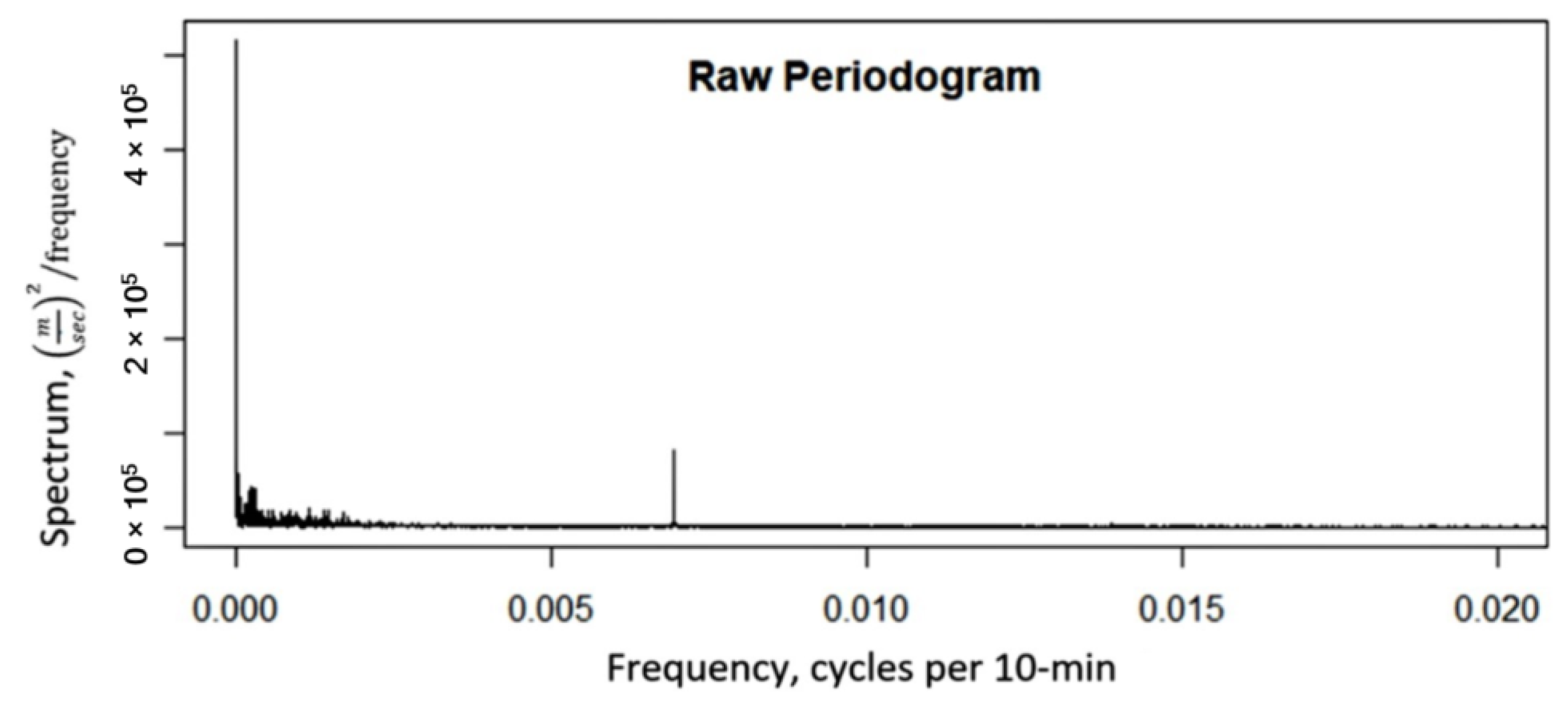
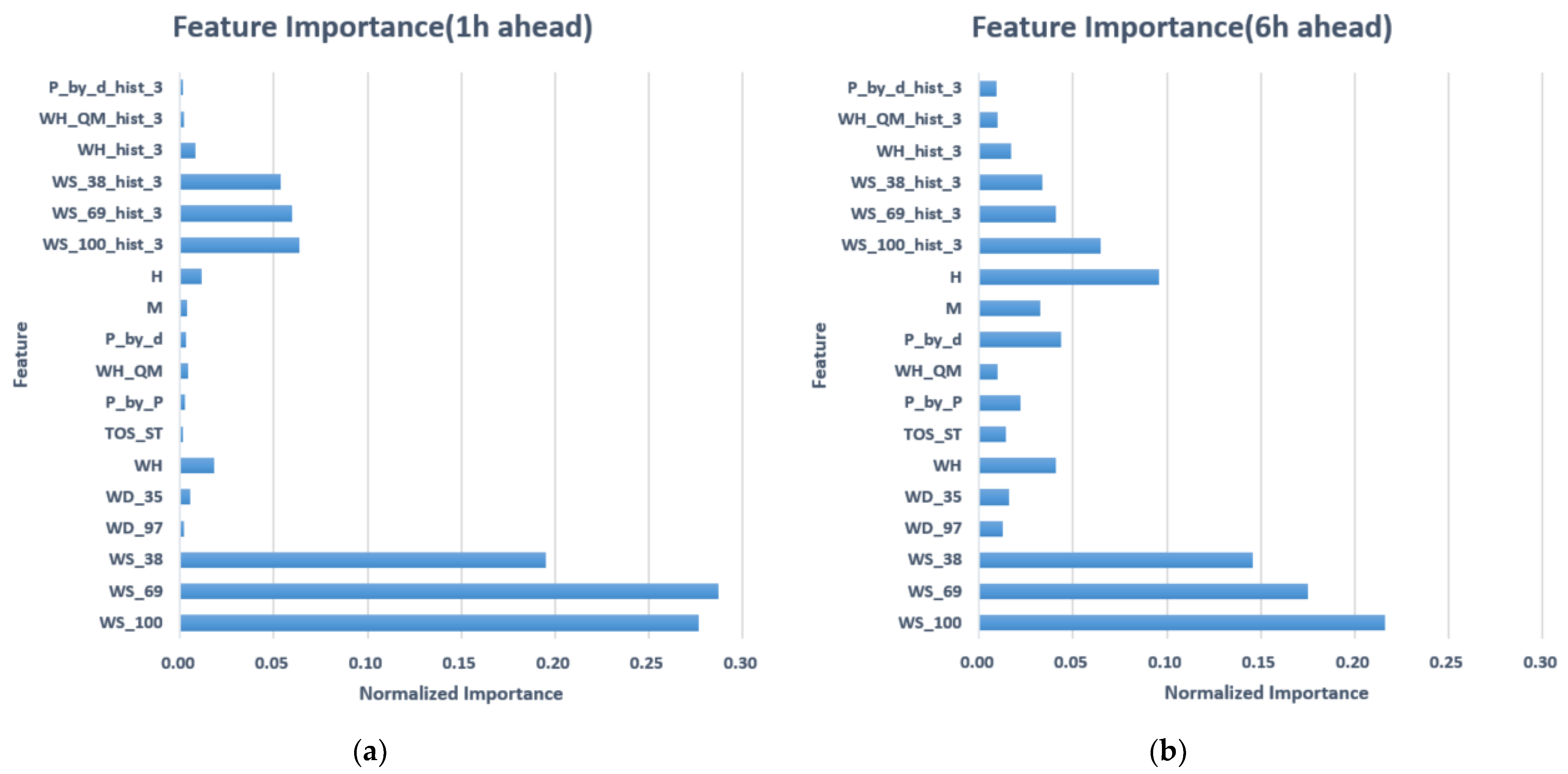
• The periodic components obtained from the time series analysis can effectively improve prediction accuracy. The improvement was more significant with the increase in lead time. At a lead time of six hours, the improvement of adding periodic components decreased the RMSE from 2.78 to 2.23 (accounting for a 44% improvement made by the random forest model, see Table 3). The diurnal variation was more evident than the monthly variation, as shown in the periodogram (Figure 4), which is consistent with the relative intensity of feature importance (Figure 6).
• Due to the significant effect of periodic components, the improvement by adding historical observation data (e.g., HS1, HS2, HS3) was very limited.
• With an increase in lead time, space-varying features (e.g., P_by_P, P_by_d) became more important. Eventually, they may have become as important as those space-fixed features (e.g., WH, WH_QM), which were more important at first.
• The atmospheric stability (e.g., TOS_ST, WSH) made quite apparent contributions. Based on our results, we suggest that the temperature difference (TOS_SH) replaces the difference in wind speed (WSH). Apart from the equivalent effect, the availability and accuracy of the former were better.
• By implementing feature engineering techniques, the RF model achieved a higher accuracy than a typical ANN model. In addition, we can extract important features from the feature importance analysis in the RF model. The important features extracted may be used in a more complicated model or integrated with the physical model in the future to improve the prediction accuracy.
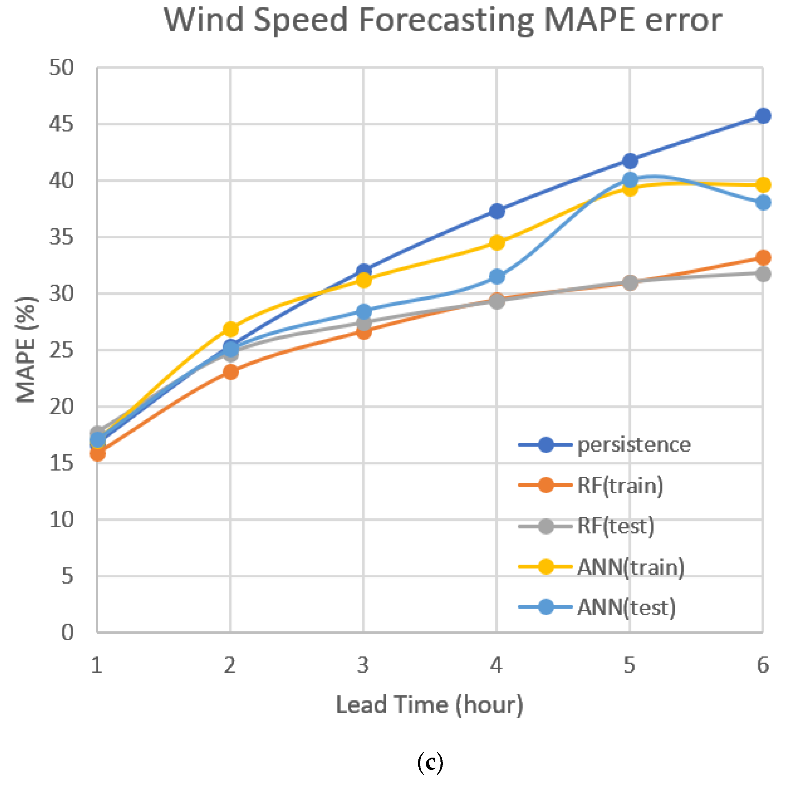
• As shown in Table 5, with a lead time of one hour, the MAPE of the RF (test) was worse than that of the persistence model, but the RMSE and MAE of the RF (test) were better than that of the persistence model. These may have been caused by error distribution. In the prediction of the RF model, there may have been larger absolute errors in the low wind speed interval, resulting in a larger MAPE obtained by dividing by the low wind speed (small denominator).

5. Conclusions

Considering the computation time and cost, statistical models are usually used for short-term forecasting. Machine learning is especially suitable for nonlinear and complex systems. In this study, the random forest method was used to develop a short-term forecasting model for wind speed in the coastal area of central Taiwan. In addition to the input features that are generally used, such as wind speed, wind direction, air pressure, and air temperature, features representing spatial and temporal variation were added to improve the accuracy of the prediction. The prediction model we developed outperformed the persistence model and the classical neural network model. Several conclusions can be drawn as follows:

• The wind speed and direction at the same measuring location are the most important features when the lead time is short.
• As the lead time increases, the importance of the spatial and temporal variation features will gradually increase. The importance of the time-varying features will be higher than that of space-varying features.
• The periodic components in the time series data could significantly improve prediction accuracy. The magnitude of the periodic components in the periodogram agrees with their importance.
• The impact of atmospheric stability is significant. Based on the availability and accuracy of the data, it is recommended to replace the difference in wind speed at different heights of the met mast with the difference in the air and sea temperatures measured by the buoy as a feature.
• The wave height measured by the buoys arranged along the coastline helps improve the accuracy of wind speed prediction because of the correlation between waves and winds.
• The air pressure difference measured by the buoys and weather stations along and across the prevailing wind direction helps to improve the accuracy of wind speed prediction.
• The weather and geography vary from place to place, along with the effectiveness of new features. However, in the area of interest, the more distinct the prevailing wind direction, the higher the air–sea temperature difference, and the more apparent diurnal variation and monthly variation, the greater the effects expected.

Most of the time, the weather conditions vary gently. If steeper variations want to be obtained to achieve higher accuracy, using only historical data is inadequate. Incorporating the prediction of physical models into a statistical model is a promising approach to improve the prediction accuracy, which is also the direction we will proceed. Therefore, in the future, we will not only keep investigating new valuable features but also try to develop hybrid models to incorporate physical models (e.g., WRF), statistical (ML or FDA) models, and new features for enhancing the accuracy of wind speed prediction.

References

1. Gielen, D.; Boshell, F.; Saygin, D.; Bazilian, M.D.; Wagner, N.; Gorini, R. The role of renewable energy in the global energy transformation. Energy Strategy Rev. 2019, 24, 38–50. [Google Scholar] [CrossRef]
2. Global Wind Atlas. The Global Wind Atlas is A free, Web-Based Application Developed to Help Policymakers, Planners, and Investors Identify High-Wind Areas for Wind Power Generation Virtually Anywhere in the World, and then Perform Preliminary Calculations. Available online: https://globalwindatlas.info/en/area/Taiwan. (accessed on 28 December 2022).
3. Offshore Wind-Power Generation. 13 June 2019. Available online: https://english.ey.gov.tw/News3/9E5540D592A5FECD/34ff3d6b-412e-458d-afe9-01737d2da52d (accessed on 1 November 2020).
4. MOEA Plans a New Target to Develop Further 10 GW of Offshore Wind Capacity Between 2026 to 2035—Anticipation of a Price Drop below the Average Consumer Price. 6 January 2020. Available online: https://www.moeaboe.gov.tw/ECW/english/news/News.aspx?kind=6&menu_id=958&news_id=16566 (accessed on 1 November 2020).
5. Soman, S.S.; Zareipour, H.; Malik, O.; Mandal, P. A review of wind power and wind speed forecasting methods with different time horizons. In Proceedings of the North American Power Symposium 2010, Arlington, TX, USA, 26–28 September 2010; IEEE: Piscataway, NJ, USA, 2010. [Google Scholar]
6. Jung, J.; Broadwater, R.P. Current status and future advances for wind speed and power forecasting. Renew. Sustain. Energy Rev. 2014, 31, 762–777. [Google Scholar] [CrossRef]
7. Chai, S.; Xu, Z.; Lai, L.L.; Wong, K.P. An overview on wind power forecasting methods. In Proceedings of the 2015 International Conference on Machine Learning and Cybernetics (ICMLC), Guangzhou, China, 12–15 July 2015; IEEE: Piscataway, NJ, USA, 2015. [Google Scholar]
8. Ramsay, J.O.; Dalzell, C. Some tools for functional data analysis. J. R. Stat. Soc. Ser. B Methodol. 1991, 53, 539–561. [Google Scholar] [CrossRef]
9. Ullah, S.; Finch, C. Applications of functional data analysis: A systematic review. BMC Med. Res. Methodol. 2013, 13, 43. [Google Scholar] [CrossRef] [PubMed] [Green Version]
10. Wang, J.-L.; Chiou, J.-M.; Müller, H.-G. Functional data analysis. Annu. Rev. Stat. Its Appl. 2016, 3, 257–295. [Google Scholar] [CrossRef] [Green Version]
11. Shah, I.; Lisi, F. Forecasting of electricity price through a functional prediction of sale and purchase curves. J. Forecast. 2020, 39, 242–259. [Google Scholar] [CrossRef]
12. Zou, Y.; Su, B.; Chen, Y. Nonparametric Functional Data Analysis for Forecasting Container Throughput: The Case of Shanghai Port. J. Mar. Sci. Eng. 2022, 10, 1712. [Google Scholar] [CrossRef]
13. Shah, I.; Jan, F.; Ali, S. Functional data approach for short-term electricity demand forecasting. Math. Probl. Eng. 2022, 2022, 6709779. [Google Scholar] [CrossRef]
14. Kutrolli, G.; Benth, F.E. An Application of Functional Data Analysis to Forecast Weather Variables. 27 September 2019. Available online: https://ssrn.com/abstract=3766459 (accessed on 28 December 2022).
15. Ghumman, A.R.; Ateeq-ur-Rauf AU, R.; Haider, H.; Shafiquzamman, M. Functional data analysis of models for predicting temperature and precipitation under climate change scenarios. J. Water Clim. Change 2020, 11, 1748–1765. [Google Scholar] [CrossRef]
16. Jørgensen, K.L.; Shaker, H.R. Wind power forecasting using machine learning: State of the art, trends and challenges. In Proceedings of the 2020 IEEE 8th International Conference on Smart Energy Grid Engineering (SEGE), Oshawa, ON, Canada, 12–14 August 2020; IEEE: Piscataway, NJ, USA, 2020. [Google Scholar]
17. Lahouar, A.; Slama, J.B.H. Hour-ahead wind power forecast based on random forests. Renew. Energy 2017, 109, 529–541. [Google Scholar] [CrossRef]
18. Shen, W.; Jiang, N.; Li, N. An EMD-RF based short-term wind power forecasting method. In Proceedings of the 2018 IEEE 7th Data Driven Control and Learning Systems Conference (DDCLS), Enshi, China, 25–28 May 2018; IEEE: Piscataway, NJ, USA, 2018. [Google Scholar]
19. Demolli, H.; Dokuz, A.S.; Ecemis, A.; Gokcek, M. Wind power forecasting based on daily wind speed data using machine learning algorithms. Energy Convers. Manag. 2019, 198, 111823. [Google Scholar] [CrossRef]
20. Januschowski, T.; Wang, Y.; Torkkola, K.; Erkkilä, T.; Hasson, H.; Gasthaus, J. Forecasting with trees. Int. J. Forecast. 2022, 38, 1473–1481. [Google Scholar] [CrossRef]
21. Optis, M.; Perr-Sauer, J. The importance of atmospheric turbulence and stability in machine-learning models of wind farm power production. Renew. Sustain. Energy Rev. 2019, 112, 27–41. [Google Scholar] [CrossRef]
22. Hanifi, S.; Liu, X.; Lin, Z.; Lotfian, S. A critical review of wind power forecasting methods—Past, present and future. Energies 2020, 13, 3764. [Google Scholar] [CrossRef]
23. Cadenas, E.; Rivera, W. Short term wind speed forecasting in La Venta, Oaxaca, México, using artificial neural networks. Renew. Energy 2009, 34, 274–278. [Google Scholar] [CrossRef]
24. Wang, Y.; Wu, L. On practical challenges of decomposition-based hybrid forecasting algorithms for wind speed and solar irradiation. Energy 2016, 112, 208–220. [Google Scholar] [CrossRef] [Green Version]
25. Cadenas, E.; Rivera, W. Wind speed forecasting in three different regions of Mexico, using a hybrid ARIMA–ANN model. Renew. Energy 2010, 35, 2732–2738. [Google Scholar] [CrossRef]
26. Cadenas, E.; Rivera, W.; Campos-Amezcua, R.; Heard, C. Wind speed prediction using a univariate ARIMA model and a multivariate NARX model. Energies 2016, 9, 109. [Google Scholar] [CrossRef] [Green Version]
27. Kira, K.; Rendell, L.A. A practical approach to feature selection. In Machine Learning Proceedings; Elsevier: Amsterdam, The Netherlands, 1992; pp. 249–256. [Google Scholar]
28. Piramuthu, S. Evaluating feature selection methods for learning in data mining applications. Eur. J. Oper. Res. 2004, 156, 483–494. [Google Scholar] [CrossRef]
29. Guo, Z.; Zhao, W.; Lu, H.; Wang, J. Multi-step forecasting for wind speed using a modified EMD-based artificial neural network model. Renew. Energy 2012, 37, 241–249. [Google Scholar] [CrossRef]
30. Wang, S.; Zhang, N.; Wu, L.; Wang, Y. Wind speed forecasting based on the hybrid ensemble empirical mode decomposition and GA-BP neural network method. Renew. Energy 2016, 94, 629–636. [Google Scholar] [CrossRef]
31. Jursa, R. Variable selection for wind power prediction using particle swarm optimization. In Proceedings of the 9th Annual Conference on Genetic and Evolutionary Computation, London, UK, 7–11 July 2007. [Google Scholar]
32. Gupta, R.; Kumar, R.; Bansal, A. Selection of Input Variables for the Prediction of Wind Speed in Wind Farms Based on Genetic Algorithm. Wind Eng. 2011, 35, 649–660. [Google Scholar] [CrossRef]
33. Jursa, R.; Rohrig, K. Short-term wind power forecasting using evolutionary algorithms for the automated specification of artificial intelligence models. Int. J. Forecast. 2008, 24, 694–709. [Google Scholar] [CrossRef]
34. Salcedo-Sanz, S.; Pastor-Sánchez, A.; Prieto, L.; Blanco-Aguilera, A.; García-Herrera, R. Feature selection in wind speed prediction systems based on a hybrid coral reefs optimization–Extreme learning machine approach. Energy Convers. Manag. 2014, 87, 10–18. [Google Scholar] [CrossRef]
35. Senthil Kumar, P.; Lopez, D. Feature selection used for wind speed forecasting with data driven approaches. J. Eng. Sci. Technol. Rev. 2015, 8, 124–127. [Google Scholar] [CrossRef]
36. Li, F.; Ren, G.; Lee, J. Multi-step wind speed prediction based on turbulence intensity and hybrid deep neural networks. Energy Convers. Manag. 2019, 186, 306–322. [Google Scholar] [CrossRef]
37. Vassallo, D.; Krishnamurthy, R.; Fernando, H. Decreasing wind speed extrapolation error via domain-specific feature extraction and selection. Wind Energy Sci. 2020, 5, 959–975. [Google Scholar] [CrossRef]
38. Zhu, Q.; Chen, J.; Shi, D.; Zhu, L.; Bai, X.; Duan, X.; Liu, Y. Learning temporal and spatial correlations jointly: A unified framework for wind speed prediction. IEEE Trans. Sustain. Energy 2019, 11, 509–523. [Google Scholar] [CrossRef]
39. Breiman, L. Random forests. Mach. Learn. 2001, 45, 5–32. [Google Scholar] [CrossRef] [Green Version]
40. Cutler, A.; Cutler, D.R.; Stevens, J.R. Random Forests. In Ensemble Machine Learning: Methods and Applications; Zhang, C., Ma, Y., Eds.; Springer US: Boston, MA, USA, 2012; pp. 157–175. [Google Scholar]
41. Hastie, T.; Tibshirani, R.; Friedman, J. The Elements of Statistical Learning: Data Mining, Inference, and Prediction; Springer Science & Business Media: Berlin, Germany, 2009. [Google Scholar]
42. Bishop, C.M. Neural Networks for Pattern Recognition; Oxford University Press: Oxford, UK, 1995. [Google Scholar]
43. Lippmann, R. An introduction to computing with neural nets. IEEE ASSP Mag. 1987, 4, 4–22. [Google Scholar] [CrossRef]
44. Mohandes, M.A.; Rehman, S.; Halawani, T. A neural networks approach for wind speed prediction. Renew. Energy 1998, 13, 345–354. [Google Scholar] [CrossRef]
45. Madsen, H.; Pinson, P.; Kariniotakis, G.; Nielsen, H.A.; Nielsen, T.S. Standardizing the Performance Evaluation of Short-Term Wind Power Prediction Models. Wind Eng. 2005, 29, 475–489. [Google Scholar] [CrossRef] [Green Version]
46. Cheng, K.-S.; Ho, C.-Y.; Teng, J.-H. Wind and Sea Breeze Characteristics for the Offshore Wind Farms in the Central Coastal Area of Taiwan. Energies 2022, 15, 992. [Google Scholar] [CrossRef]
47. Stull, R.B. An Introduction to Boundary Layer Meteorology; Springer Science & Business Media: Berlin, Germany, 1988; Volume 13. [Google Scholar]
48. Cheng, K.-S.; Ho, C.-Y.; Teng, J.-H. Wind Characteristics in the Taiwan Strait: A Case Study of the First Offshore Wind Farm in Taiwan. Energies 2020, 13, 6492. [Google Scholar] [CrossRef]
49. Hasselmann, K.; Barnett, T.P.; Bouws, E.; Carlson, H.; Cartwright, D.E.; Enke, K.; Ewing, J.A.; Gienapp, H.; Hasselman, D.E.; Kruseman, P.; et al. Measurements of wind-wave growth and swell decay during the Joint North Sea Wave Project (JONSWAP). Ergaenzungsheft Zur Dtsch. Hydrogr. Z. Reihe A 1973, 12, 7–94. [Google Scholar]
Figure 1. An example of ANN architecture, which consists of 1 input layer, 2 hidden layers, and 1 output layer.
Energies 16 01374 g001
Figure 2. Wind rose at 100 m of BSMI met mast in 2019 [48].
Energies 16 01374 g002
Figure 3. (a)The position of the buoys, Wuqi station, and met mast. The green tags from north to south are the Hsin Chu, Tai Chung, and Ci Mei buoys, respectively. The blue tag is Wuqi Station, and the yellow tag is the BSMI met mast. (b) Surface observation sites around central Taiwan.
Energies 16 01374 g003
Figure 4. The periodogram of 10 min average wind speed at a 100 m height.
Energies 16 01374 g004
Figure 5. The wind speed diurnal variation patterns of individual months.
Energies 16 01374 g005
Figure 6. Feature importance of different predicting periods. (a) Feature importance of one hour ahead. (b) Feature importance of 6 h ahead.
Energies 16 01374 g006
Figure 7. RMSEs of different models, which consist of different features.
Energies 16 01374 g007
Figure 8. The RMSE comparison of ANN with simple features and all features (new features included).
Energies 16 01374 g008
Figure 9. The comparisons among the performances of the persistence model, RF model, and ANN model. (a) Comparison of RMSE, (b) comparison of MAE, (c) comparison of MAPE.
Energies 16 01374 g009aEnergies 16 01374 g009b