The Impact of Transmission Line Modeling on Lightning Overvoltage

Abstract

In most of the work that investigates the backflashover phenomenon due to direct lightning strikes, using EMT-type simulators, transmission lines are represented by the J. Marti model and the ground effect is computed employing J. R. Carson’s formulations. Thus, the ground displacement current is neglected, the line voltage definition corresponds to the wire potential formulation, and soil resistivity is considered frequency-independent. These considerations can lead to erroneous measurements of the occurrences of the backflashover phenomenon in the insulator strings of transmission line. In this sense, this paper presents a systematic sensitivity analysis study of lightning overvoltage in insulator strings considering more physically consistent models of the transmission line, which consider the displacement current, ground admittance correction, rigorous voltage definition, and frequency-dependent soil parameters. According to the results, for the case study, transmission line parameters modeling can present a maximum percentual difference of around 71.54%, considering the frequency range of first strokes. This difference leads to a percent difference of around 5.25% in the maximum overvoltage across the insulator strings. These differences confirm that the occurrence or not of backflashover in the insulator strings, including the disruption time, are sensitive to the line model considered.

1. Introduction

Power outages due to lightning is one of the main causes of transmission lines (TLs) shutdowns, for power systems with voltage levels up to 500 kV. To reduce the number of these shutdowns, one must understand the phenomenon that requests the TL as well as simulates it, considering adequate models to avoid either under- or over-estimation. To guarantee an adequate and consistent transmission systems outage rate, the accurate representation of the TL and grounding system is of utmost importance.

For the representation of the grounding system, precise models were implemented in the literature, such as the well-known hybrid electromagnetic model (HEM) [1]. The HEM is based on the field and circuit theories, is accurate from dc to a couple of megahertz and considers the frequency-dependent soil electrical parameters. On the other hand, in the representation of TLs the ground effect is computed employing J. R. Carson’s formulation, which neglects ground displacement current, assumes the soil electrical parameters as frequency-independent and considers that the line voltage definition corresponds to the wire potential formulation (formulation simplified). These considerations can lead to erroneous measurements of the occurrences of the backflashover phenomenon in the insulator strings of TL.

Below are mentioned some of the works reported in recent years for the representation of the TLs.

In [2,3,4,5], the TLs were modeled using the J. Marti model and the line parameters were calculated using Carson’s formulation in EMT-type simulators (ATP, EMTP-RV, PSCAD, etc.). In these works, the authors investigate overvoltages caused by direct strokes considering the frequency-dependent (FD) characteristics of ground/soil, lightning protection systems of overhead TLs, overvoltages in insulator strings considering several tower-footing grounding impulsive modeling, and lightning performance of a TL with grounding, respectively. However, Carson’s formulation considers a simple voltage definition as well as disregards the displacement current. Additionally, most of the EMT-type software do not consider soil frequency-dependence.

In [6], the soil frequency-dependence, the displacement current, imperfect earth on the shunt addmittance and the impact of several formulations to calculate the line parameters were taken into account in the transient voltages at the open-receiving end of overhead distribution lines. These transients were calculated using the numerical Laplace transform (NLT) implemented in MATLAB programming language. However, the model used to correct the soil conductivity (Longmire and Smith [7]) is limited to values bellow 1.000 $\mathrm{\Omega }$.m [8]. Moreover, the proposed methodology cannot be implemented in EMT-type software as well as does not include the rest of the power system elements (towers, grounding and insulator strings, for instance).

In [9,10], the Alipio model, which is indicated by CIGRE [8] to evaluate lighting-related studies, and Pettersson formulation to calculate transmission line modeling are used to investigated lightning-related transients in transmission lines. In these works, TL is represented in the frequency domain by its nodal admittance matrix and time domain simulations carried out using the NLT. However, this approach cannot be implemented in EMT-type softwares and does not allow the direct consideration of non-linear elements.

In [11], a modified model of the J. Marti model was presented. This was called the modified JMarti model. In this model Carson and Nakagawa formulations were used to calculate line parameters. However, only simple configurations such as single- and two-phase power distribution lines including FD soil parameters were investigated.

In [12], a multi-phase analysis was carried out, considering the Petterson formulation in the modified JMarti model. However, no other transmission element was considered, i.e., only the line response was evaluated.

In [13], the modified JMarti model with Sunde’s formulation to calculate the line parameters was used in the ATP simulator. In this work was presented a comparison of overvoltages in the phase conductors assuming the frequency dependence of soil parameters. However, only simple voltage definition in the line modeling was considered and the insulator string modeling was not discussed.

This paper aims to evaluate the impact of previous approximations in the insulator strings overvoltage since none of the aforementioned show a comparison of overvoltages along the insulator strings, considering a more rigorous voltage definition in calculating the line parameters together with a grounding system modeling in the ATP, showing in which cases a backflashover occurs. To fill this gap, this paper presents a systematic sensitivity analysis study of lightning overvoltage in insulator strings, considering more physically consistent models, which consider the displacement current, ground admittance correction, rigorous voltage definition and frequency-dependent soil parameters.

This paper is organized into five sections. After this introductory section, Section 2 presents the multiconductor transmission line modeling, the expressions for the ground return impedance and admittance matrices, and the implementation strategy in the ATP simulator. In Section 3, there is the system description, which is composed of the representations of the transmission tower, insulator strings, tower-footing grounding and lightning current. The implementation of these representations are shown in the ATP simulator. In Section 4, the results and respective sensitivity analyses are presented. Finally, in Section 5 are the conclusions.

2. Multiconductor Transmission Line Modeling

This section is divided in two parts which are: (i) calculation of line parameter—detailing the different expressions for the impedance and admittance matrices, these expressions are obtained from the different line voltage definitions presented in [9]; and (ii) TLs model and implementation strategy—detailing the TL modeling and how the calculations of line parameters are considered, through an external file, in one of the main time-domain simulators, the ATP simulator.

2.1. Calculation of Line Parameter

An overhead line, for TL modeling, can be approximately as infinitely long conductors. For instance, for the sake of representation, one can consider Figure 1 as a TL composed of two conductors, i and j, both at a constant average height, $h_i$ and $h_j$, respectively, with the radius $r_i=r_j=r$, and horizontal distance $x_{ij}$. In this case, both air and soil are characterized by its electrical permittivity (${\epsilon }_i$), conductivity (${\sigma }_i$) and magnetic permeability (${\mu }_i$) where i = 1 for air and i = 2 for the soil (both are considered homogeneous media). The propagation constant ($\gamma$) in each medium is given by ${\gamma }_i=\sqrt{j\omega {\mu }_i({\sigma }_i+j\omega {\epsilon }_i)}$, $\omega$ is the angular frequency, ${\mu }_i={\mu }_{ri}{\mu }_0$ and ${\epsilon }_i={\epsilon }_{ri}{\epsilon }_0$ where ${\mu }_{ri}$ and ${\epsilon }_{ri}$ are the relative permeability and permittivity of the ground and ${\mu }_0$ and ${\epsilon }_0$ are the permeability and permittivity of the vacuum.

The determination of the pul parameters of the line, are found through the wire voltage to ground (U) [14,15]. U can be defined through three formulations: potential, potential difference, and voltage. These formulations use the magnetic vector potential A and the electric scalar potential $\phi$ [9,15]. Here follows the three possible definitions:

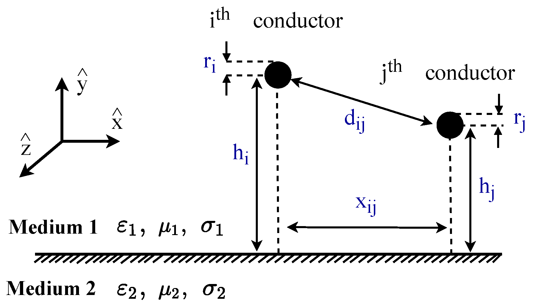
• Potential formulation: corresponds to considering a remote ground for potential reference (the electrical scalar potential being defined in relative to a remote ground). It is given by:

  $$U_i=\phi \left(x,h-r\right)$$

  (1)

  where $\phi (x,y=h-r)$ is the wire scalar potential with the reference at infinity;
• Potential difference formulation: corresponds to the potential difference between the surface of the conductor and the ground and does not consider the potential magnetic vector. This definition is given by:

  $$U_{ip}=\phi \left(x,h-r\right)-\phi \left(x,0\right)$$

  (2)

  where $\phi \left(x,0\right)$ is the ground surface potential;
• Voltage formulation: it is the most rigorous and consists in calculating the voltage between the overhead conductor and the earth surface below. In this case both electric scalar and magnetic vector potentials are considered in a vertical path. This definition is given by:

  $$U_{ii}=\phi \left(x,h-r\right)-\phi \left(x,0\right)+j\omega {\int }_0^{h-r}{A}_y\left(x,y^{\prime }\right)d{y}^{\prime }$$

  (3)

  where $A_y$ is the magnetic vector potential at direction y (see [9,14,15] for details).

The numerical solution of $\gamma$ is cumbersome and computationally inefficient [15]. To overcome such inefficiency, the so-called quasi-TEM approximation can be used [14] so the $\gamma$ is considered equal to the intrinsic propagation constant of the medium in which the wire is immersed [15]. Applying definition $U_i$, Pettersson [14] obtained (4) and (5) for calculating the pul parameters of an overhead wire. Moreover, considering the definition $U_{ip}$, Pettersson obtained (6) and (7) [14]. On the other hand, considering voltage definition $U_{ii}$, Pettersson obtained (8) and (9) [14].

It is noteworthy to comment that neglecting the ground displacement currents, $S_2$, $S_3$ and $S_4$ tend to zero. If the ground is assumed as a good conductor, it is possible to approximate $\phi \left(x,0\right)\approx$$A_y\left(x,y^{\prime }\right)\approx$ 0 and U $\approx \phi \left(x,h-r\right)$, guaranteeing electrostatic conditions. Thus, it is possible to assume that the scalar potential and the conductor voltage (with respect to the ground) are essentially the same. Otherwise, there will be a noticeable difference between the potentials [15,16].

$$Z_{Ui}=Z_{int}+\frac{j\omega {\mu }_0}{2\pi }\left\{M+S_1\right\}$$

(4)

$$Y_{Ui}=j\omega {\epsilon }_{0}2\pi {\left(M+S_2\right)}^{-1}$$

(5)

$$Z_{Uip}=Z_{int}+\frac{j\omega {\mu }_0}{2\pi }\left\{M+S_1-\left(S_2+S_3\right)\right\}$$

(6)

$$Y_{Uip}=j\omega {\epsilon }_{0}2\pi {\left(M-S_3\right)}^{-1}$$

(7)

$$Z_{Uii}=Z_{int}+\frac{j\omega {\mu }_0}{2\pi }\left\{M+S_1-\left(S_2+S_4\right)\right\}$$

(8)

$$Y_{Uii}=j\omega {\epsilon }_{0}2\pi {\left(M-S_4\right)}^{-1}$$

(9)

From the previous equations, $Z_{int}$ is the matrix that considers the internal impedance of the conductors ((diagonal matriz with the elements calculated with (10)), $M$ is a matrix whose elements are given by (11) and finally the correction terms that considers the finite conductivity effects of the soil, $S_1$, $S_2$, $S_3$ and $S_4$ are given by (12)–(15), respectively, [14,17].

$$Z_{{int}_{(i,i)}}=\frac{1}{2\pi r_i}\sqrt{\frac{j\omega {\mu }_i}{{\sigma }_i}}\frac{I_0\left(\sqrt{j\omega {\mu }_0{\sigma }_i,r_i}\right)}{I_1\left(\sqrt{j\omega {\mu }_0{\sigma }_i,r_i}\right)}$$

(10)

$$M_{\left(i,i\right)}=ln\left(\frac{2h_i}{r_i}\right);M_{\left(i,j\right)}=ln\left(\frac{D_{ij}}{d_{ij}}\right)$$

(11)

$$S_{1\left(i,j\right)}={\int }_{-\infty }^{\infty }\frac{e^{-\lambda {\ell }_{ij}}}{\lambda +u_2}cos\left(x_{ij}\lambda \right)d\lambda$$

(12)

$$S_{2\left(i,j\right)}={\int }_{-\infty }^{\infty }\frac{e^{-\lambda {\ell }_{ij}}}{n^2\lambda +u_2}cos\left(x_{ij}\lambda \right)d\lambda$$

(13)

$${S_3}_{\left(i,j\right)}={\int }_{-\infty }^{\infty }\left(\frac{e^{-\lambda {\ell }_{ij}/2}-e^{-\lambda {\ell }_{ij}}}{n^2\lambda +u_2}\right)cos\left(x_{ij}\lambda \right)d\lambda$$

(14)

$${S_4}_{\left(i,j\right)}={\int }_{-\infty }^{\infty }\frac{u_2}{\lambda }\left(\frac{e^{-\lambda {\ell }_{ij}/2}-e^{-\lambda {\ell }_{ij}}}{n^2\lambda +u_2}\right)cos\left(x_{ij}\lambda \right)d\lambda$$

(15)

where $I_0$ and $I_1$ are modified Bessel functions of first kind and orders zero and one, respectively. $D_{ij}=\sqrt{{\ell }_{ij}^2+x_{ij}^2}$ and $\ell =h_i+h_j$, $n={\gamma }_2/{\gamma }_1$ and $u_2=\sqrt{{\lambda }^2+{\gamma }_2^2-{\gamma }_1^2}$.

In [14,15], its shown that terms of $S_1$, $S_2$, $S_3$ and $S_4$ in (4)–(9) improves the pul parameters modeling by extending its validity limits, especially for frequencies in the range of tens of MHz. Equations (4) and (5) are equivalent to the integral equations proposed by Nakagawa [18] if the magnetic permeability of media 1 and 2 are equal, i.e., Nakagawa’s model takes into account only $S_1$ and $S_2$ corrections, assuming potential formulation. Further, if the ground is assumed to be a good conductor, then the displacement currents can be neglected as both $S_2$ and $S_4$ tend to zero in (8), it becomes the equation $S_1$ in (4). It can be shown that this term reduces to Carson’s integral equation [19] if ${\epsilon }_{r2}$ = 1, or to Sunde’s integral equation [20] if either ${\epsilon }_{r2}>>$ 1 or ${\gamma }_1$ = 0 are considered [21]. The fact that in Sunde’s and Carson’s equations the term $S_2$ is assumed equal to zero makes them unsuitable for broadband applications [9,14,15,21].

In this paper, only potential and voltage formulations were used, since they are the most extreme formulations (fewer and more terms in the calculation) and, as shown in [9], are the ones that can give the greatest differences.

2.2. Formulation of the Transmission Lines Model and Implementation Strategy

In the traditional JMarti’s TL model [22], the matrices characteristic impedance ($Z_c$) and propagation function ($H$) are approximated by a rational function using the Bode’s method. Roughly, the Bode’s method consists of a graphical technique based on Bode’s diagram. This line model is usually incorporated in popular EMT-like software [23].

In order to evaluate Pettersson’s formulations for the line parameters a “modified JMarti model” is considered. This implementation was proposed in [11] and allows us to extend the capacity of the JMarti model in ATP to include more general equations in the calculation of soil parameters, as well as frequency-dependent soil parameters. However, in [11], only simple configurations distribution lines are investigated, including FD soil parameters. In addition, the line parameters formulation considered were the ones proposed in [18,19], which is a simplified formulation when compared with the Pettersson proposal. Furthermore, in [11], the effect of the soil admittance correction was neglected in the calculations and, also, it is not clear how the real poles and residues of $Z_c$ and $H$ were obtained. Here, we extend the implementation to be used in a three-phase line, use more complete line parameter calculation formulations, and use a methodology to obtain the real poles and residues of $Z_c$ and $H$ with good accuracy.

The implementation of the modified JMarti model employs the VF method [24] to fit the matrices $Z_c$ and $H$. This implementation can also include the frequency dependence of soil parameters in the ground return impedance and ground admittance correction calculation. For this implementation in the ATP-software, the complex poles of $Z_c$ and $H$ obtained with the VF method are replaced by real poles based on the non-predominance of complex poles for smooth functions and the fitting procedure must respect the conditions established in [25]. The performances of the Bode’s and VF’s methods were compared in [25], where lower deviations in the $Z_c$ and $H$ are obtained using the VF method.

The implementation of modified JMarti model in ATP follows a strategy that combines the use of MATLAB and ATP as shown in Figure 2. Initially, the user enters the TL data in the MATLAB, which is responsible for calculating the line parameters, the time delays, a real transformation matrix and the functions $Z_c$ and $H$ plus their fitting.

In the end, the poles and residues of $Z_c$ and $H$, the minimum time delays and a real transformation matrix are written in the form of a .pch file that is interpreted by ATP as JMarti type TL model which are included in the ATP. It is important to highlight that a code used to generate .pch files, considering a specific set of data (real poles and residues), was presented in [11].

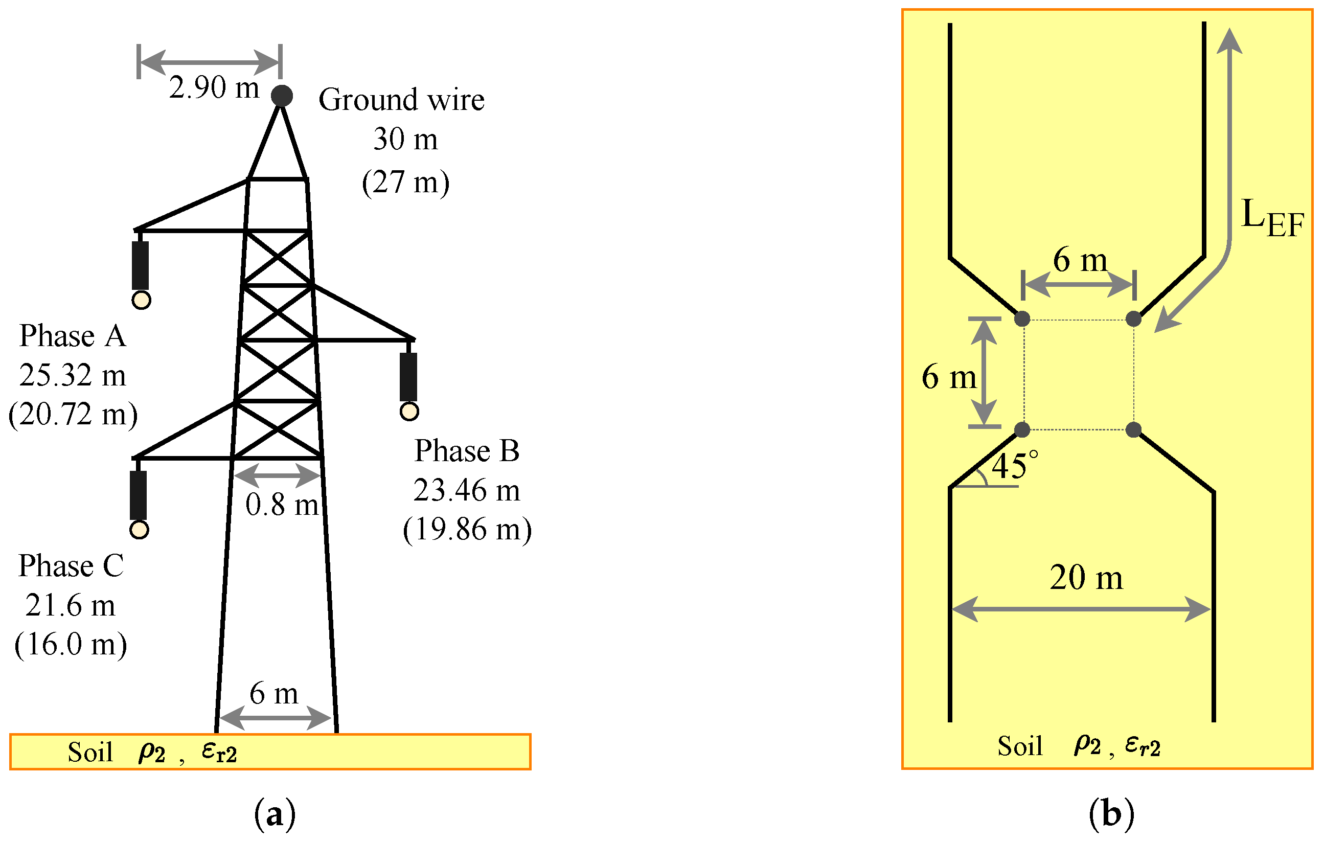
3. System Description

To assess the TL impact on lightning overvoltages, a 138 kV system is considered, and the simulation is composed of five towers and six spans of 380 m. The results are obtained considering the lightning striking the central tower. It is important to highlight that, for lightning studies, since the current front-time is fast, the consideration of more than five towers is unnecessary since there is not enough time for the traveling wave to present an impact on the lightning overvoltage across the insulator strings.

The tower data are illustrated in Figure 3a, where the values within parentheses are midspan heights. This TL is composed of the phase conductors (A, B and C), and one ground wire (GW) whose data is shown in the

Table 1. Conductors applied to the 138-kV TL.

	Phase	Outer Radius (cm)	DC Resistance (Ω/km)
Phase cables (ACSR)	A B C	1.60 1.60 1.60	0.063 0.063 0.063
Ground wire (3/8” EHS)	GW	0.79	0.500

. Figure 3b illustrates a typical counterpoise arrangement of the TL grounding. It consists of four counterpoise cables and each one starting from a tower foot. The counterpoises are buried at a depth of 0.5 m and have a radius of 15 mm. The modeling of each component are briefly described hereafter.

3.1. Frequency Dependence of Soil Parameters

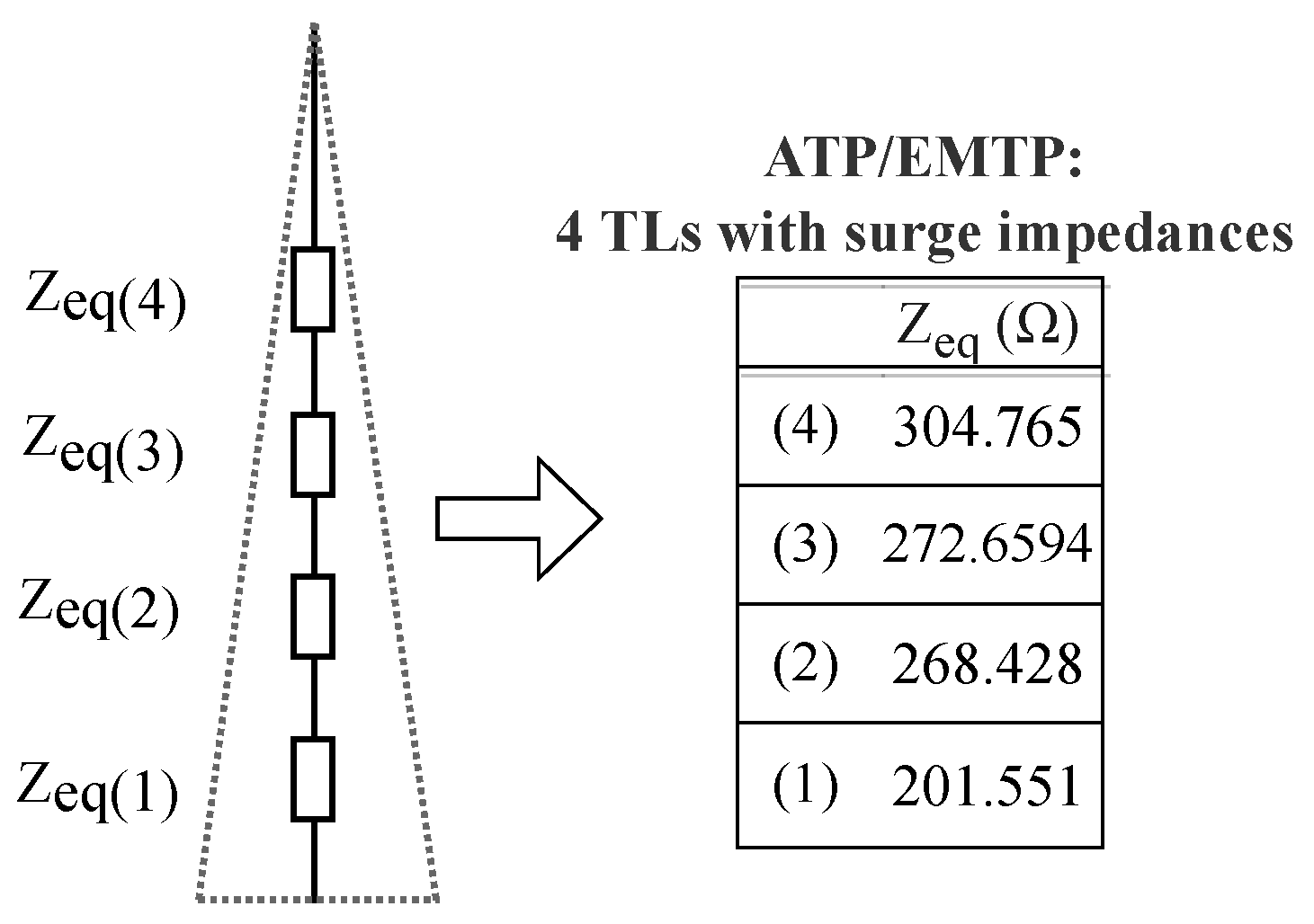
There are several models that considers the soil parameters as frequency dependent [26]. These models are expressed based on either laboratorial or in situ experimental data. Among all models that consider the soil parameters frequency dependence, one that is noteworthy is the Alipio–Visacro model [27]. It was obtained considering in situ experiments and was recently recommended by [8] for lightning-related studies. Moreover, this model satisfies causality. For these reasons, this model is considered in this paper. In (16) and (17) are illustrated the formulations of the model.

$${\sigma }_2\left(f\right)={\sigma }_0+{\sigma }_0\times h\left({\sigma }_0\right){\left(f\times {10}^{-6}\right)}^{\xi }$$

(16)

$${\epsilon }_{r2}\left(f\right)={\epsilon }_{r\infty }+\frac{tan(\pi \xi /2)\times {10}^{-3}}{2\pi {\epsilon }_0{\left({10}^6\right)}^{\xi }}{\sigma }_0\times h\left({\sigma }_0\right)f^{\xi -1}$$

(17)

where ${\sigma }_2$ is the soil conductivity in mS/m (or resistivity ${\rho }_2$ = ${\sigma }_2^{-1}$), ${\sigma }_0$ is the DC conductivity in mS/m, ${\epsilon }_{r2}$ is the relative permittivity in F/m, ${\epsilon }_{r\infty }$ is the relative permittivity at higher frequencies, ${\epsilon }_0$ is the vacuum permittivity in F/m and f is the frequency in Hz.

According to [27], the following parameters are recommended in (16) and (17) to obtain mean results for the frequency variation of ${\sigma }_2$ and ${\epsilon }_{r2}:\xi$ = 0.54, ${\epsilon }_{r\infty }$ = 12 and h(${\sigma }_0$) = 1.26 $\times {\sigma }_0^{-0.73}$.

3.2. Tower Model

The tower modeling considered in this paper is based on lossless single-phase TL, since it is commonly used for lighting-related phenomena [28]. To take into account the geometric variations of the structure, a widely used technique is to segment the tower and represent its section by a lossless line. In this paper, each surge impedance (for each section) is calculated considering the revised Jordan’s formula, as proposed in [29]. This methodology permits the calculation of both self and mutual surge impedances of vertical multiconductor systems leading to a simplified representation of towers using the theory of TLs.

In this particular study, the tower was divided into four sections, according to the schematic diagram shown in Figure 4, and the propagation velocity was considered equal to 80% of light speed. This modeling technique has provided reliable results in lightning transient studies [29]. The characteristic impedance of each segment is also presented in the same figure.

3.3. Insulator Strings

The insulation strength depends on the waveform of the applied voltage. Considering lightning, to determine whether or not the line insulation breakdown may be evaluated using the following approaches:

• Voltage–time curves [30];
• Disruptive effect method [31];
• Physicals models [32,33].

In this work, the Disruptive Effect method (DE method) approach has been adopted since it is easy to obtain its parameters and it also presents excellent accuracy [34].

The DE method concept is based on the idea of the existence of an integral disruptive effect (DE) that, if voltage surge across an insulator string exceeds this value, a disruptive discharge will probably occur [34]. The disruptive effect associated with a voltage waveform is determined by

$$\mathrm{DE}={\int }_{t_0}^{t_a}{\left(v\left(t\right)-V_0\right)}^{k}dt$$

(18)

where v(t) is the voltage across the insulator string, $V_0$ is the voltage threshold that begins the rupture process, $t_0$ is the time value when v(t) exceeds $V_0$, k is a empirical factor and DE is the variable called “disruptive effect". For a typical 138 kV line with Critical FlashOver voltage (CFO) = 650 kV, DE method constants can be obtained according to [34]: ${\mathrm{DE}}_{\mathrm{c}}$ = 1.1506 (CFO)${}^k$; k = 1.36; $V_0$ = 0.77 (CFO) = 500.5 kV.

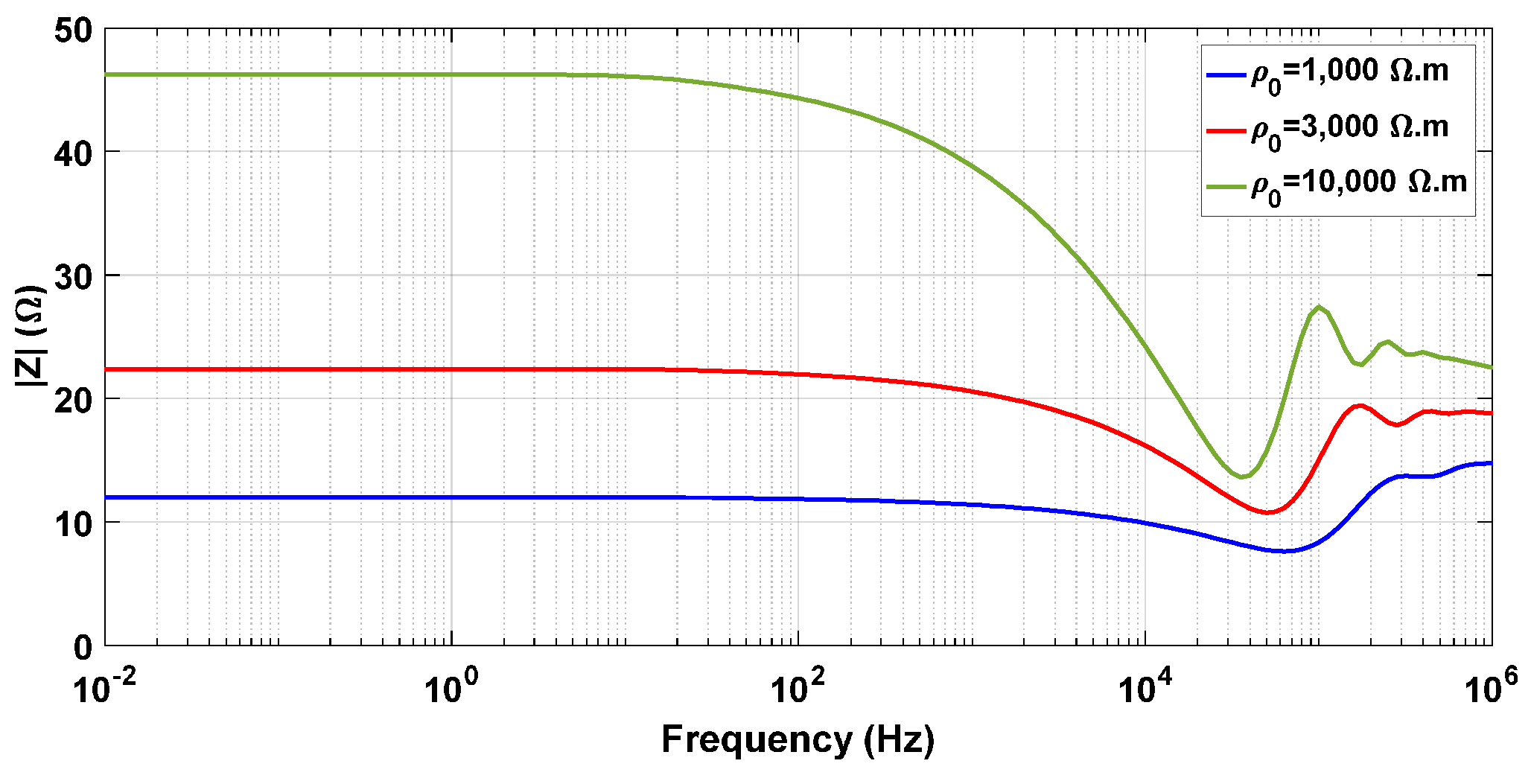
3.4. Tower-Footing Grounding

The grounding system modeling is fundamental to correctly evaluating the backflashover occurrence due to direct strikes when it occurs in both shield wire or tower. Therefore, to calculate the grounding impedance, the Hybrid Electromagnetic Model (HEM) with frequency-dependent soil electrical parameters is used [1].

Thus, the impedance Z($\omega$) is determined in a frequency range from DC to several MHz. After determining the harmonic impedance Z($\omega$), a pole-residue model of the associated admittance Y($\omega$) = 1/Z($\omega$) is obtained using the VF method [24]. After that, an electrical network is obtained that represents the frequency response of the grounding from the passive pole residue model corresponding to the grounding admittance.

In this paper, the low-frequency soil resistivities (${\rho }_0$) considered are 1000 $\mathrm{\Omega }.$m, 3000 $\mathrm{\Omega }.$m and 10,000 $\mathrm{\Omega }.$m. For these resistivities, the effective length (${\mathrm{L}}_{\mathrm{EF}}$) of a counterpoise wire (see Figure 3b) was selected according to ${\rho }_0$, using HEM and lightning first stroke to estimate it. The data can be found in

Table 2. Effective length of the counterpoise wires for first negative strokes.

${\mathit{\rho }}_0$ (Ω.m)	1000	3000	10,000
${\mathrm{L}}_{\mathrm{EF}}$ (m)	55	100	180

. To illustrate the grounding harmonic impedance, Figure 5 shows magnitude of the harmonic grounding impedance for all data from Table 2. As can be seen, for low frequencies up to a certain frequency, the grounding impedance presents a purely resistive behavior where its magnitude decreases as the soil resistivity decreases. At a certain frequency the harmonic impedance becomes inductive or capacitive, depending on the frequency range.

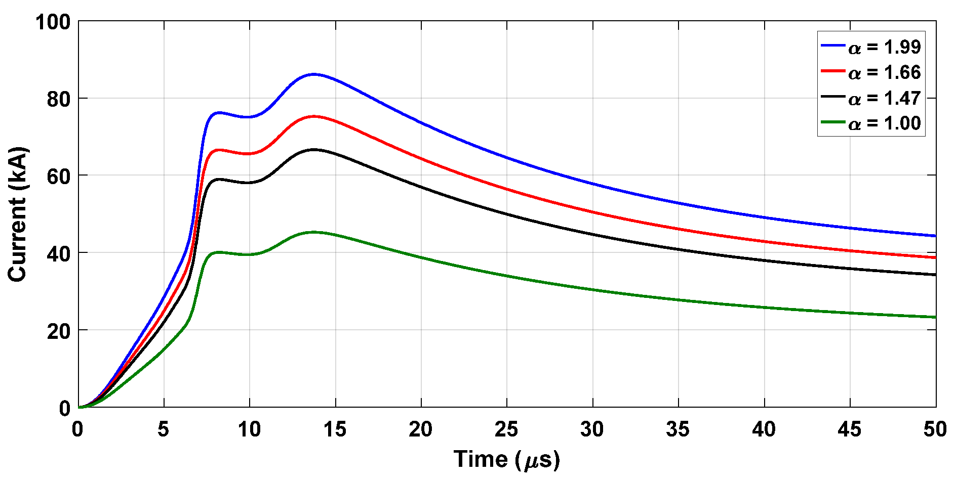
3.5. Lightning Current

The lightning current waveform that strikes the transmission tower top is represented by the sum of seven Heidler functions, according to [35,36]. The current associated with the first return strokes is considered. Its typical parameters (current peaks, front times, etc.) are the medians of measurements performed at the Morro do Cachimbo Station, Brazil. In this paper, a scalable format of the waveshape was considered, especially with regard to the amplitude [37,38]. To achieve that, an $\alpha$ multiplier parameter was used to adjust the lightning current. Figure 6 shows different waveforms considering four values, $\alpha$ = 1.00 (median value), $\alpha$ = 1.47, $\alpha$ = 1.66 and $\alpha$ = 1.99.

Additional details can be found in [37,38]. A 400 $\mathrm{\Omega }$ resistor was inserted in parallel to the current source to represent the lightning channel.

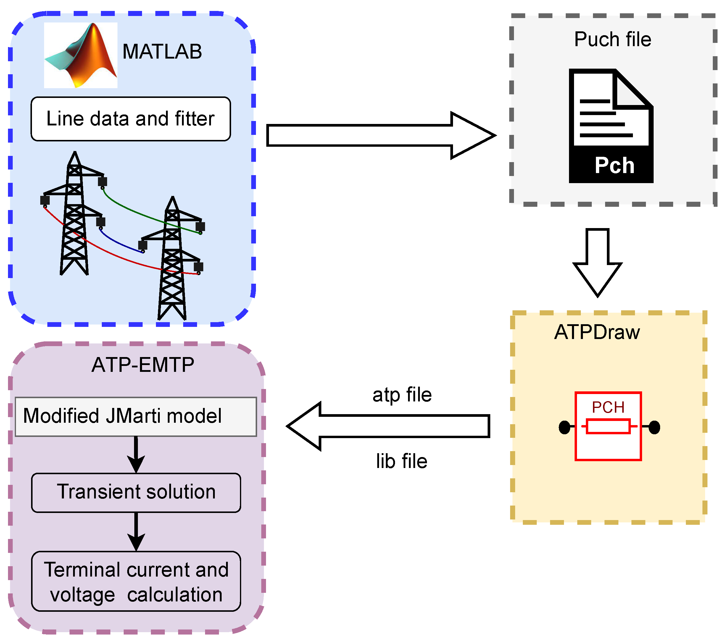
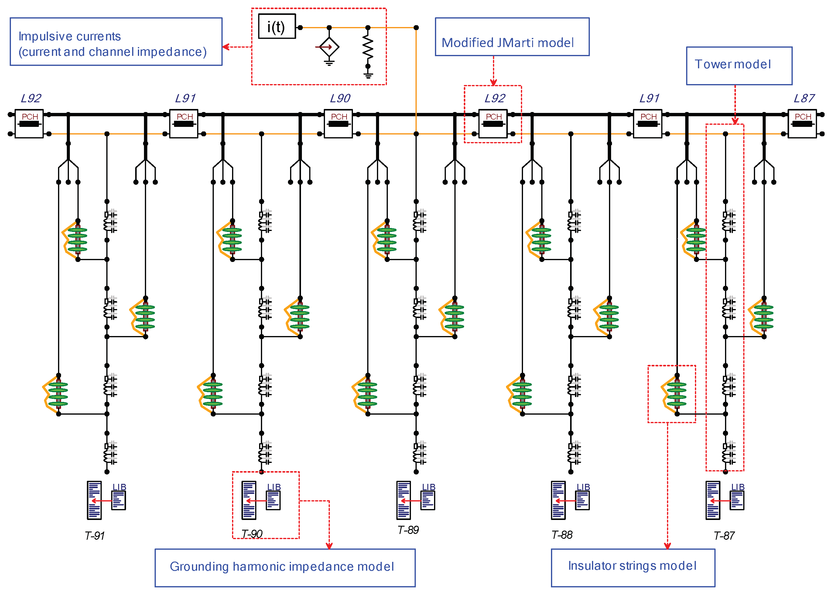
3.6. System Implementation in ATP

Figure 7 presents the whole system implemented in ATP, according to the models described in the previous subsections. It is additionally worth noting that line span, insulator strings and grounding system harmonic impedance were implemented in the PCH, MODELS and LIB blocks, respectively.

4. Results

In order to compare the line parameters and the lightning overvoltages arising from the TL modeling (see Section 2),

Table 3. Types of modeling representations.

Representation	TL Model	Formulation	Soil for TL
1	JMarti	Carson	${\rho }_0$
2	Modified JMarti	Pettersson ${\mathrm{U}}_{\mathrm{i}}$	${\rho }_0$, ${\epsilon }_{r2}$
3	Modified JMarti	Pettersson ${\mathrm{U}}_{\mathrm{i}}$	${\rho }_2$(f), ${\epsilon }_{r2}$(f)
4	Modified JMarti	Pettersson ${\mathrm{U}}_{\mathrm{ii}}$	${\rho }_0$, ${\epsilon }_{r2}$
5	Modified JMarti	Pettersson ${\mathrm{U}}_{\mathrm{ii}}$	${\rho }_2$(f), ${\epsilon }_{r2}$(f)

summarizes five different representations, chosen to carry out sensitivity analyzes.

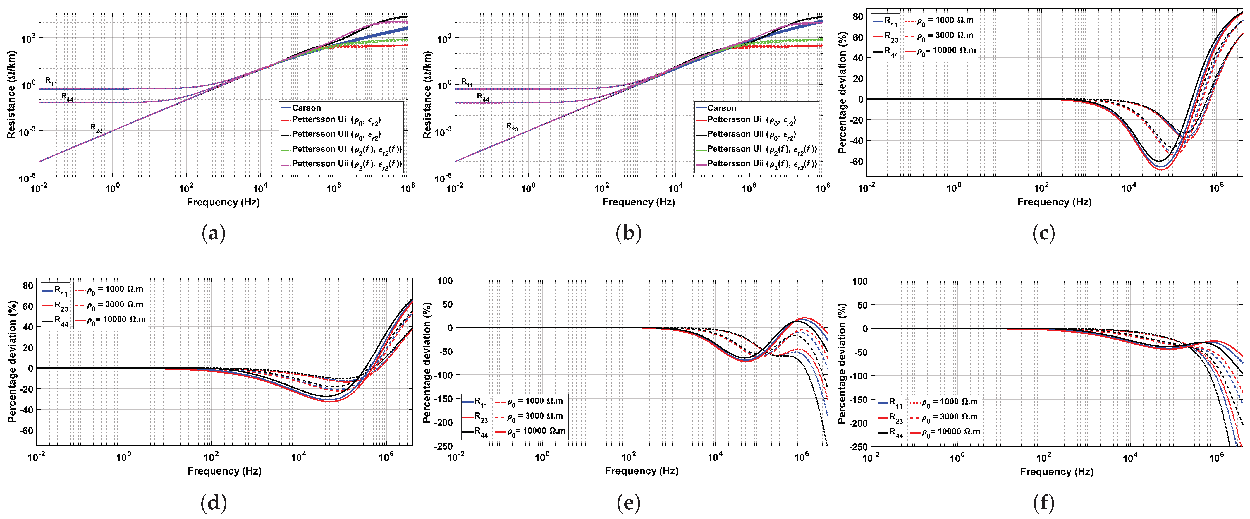
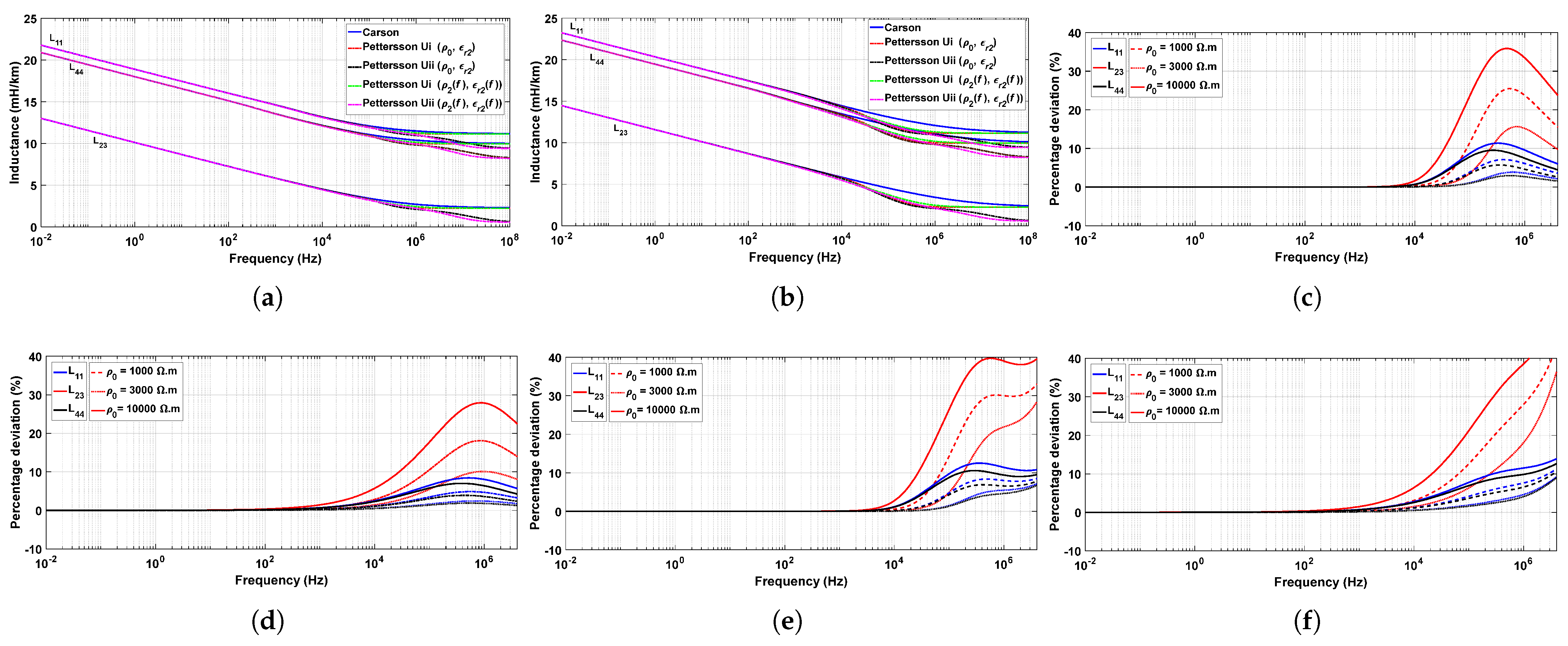
4.1. Behavior of Line Parameters

The matrices $R$, $L$ and $C$ can be expressed as follows

$$R\left(f\right)=\Re \left\{Z\left(2\pi f\right)\right\}$$

(19)

$$L\left(f\right)=\frac{\Im \left\{Z\left(2\pi f\right)\right\}}{2\pi f}$$

(20)

$$C\left(f\right)=\frac{\Im \left\{Y\left(2\pi f\right)\right\}}{2\pi f}$$

(21)

where ℜ and ℑ stand for the real and imaginary parts of the matrices $Z$ and $Y$ (equivalent series and shunt parameters). The conductance is neglected in this analysis.

The procedure to compute the matrices $Z$ and $Y$ are described in [39], where $R$, $L$ and $C$ are calculated using:

• Carson (CA) [19];
• Pettersson (PE) [14].

To compute these line parameters, three different soils were used with ${\rho }_0$ of 1000 $\mathrm{\Omega }$.m, 3000 $\mathrm{\Omega }$.m and 10,000 $\mathrm{\Omega }$.m for a frequency range of 0.01 Hz to 100 MHz. Furthermore, the percentage deviation $\delta$(%) is given by

$${\delta }_{R,L,C}\left(f\right)=\frac{p_{\mathrm{ij}}^{\mathrm{CA}}-p_{\mathrm{ij}}^{\mathrm{PE}}}{p_{\mathrm{ij}}^{\mathrm{CA}}}\times 100\%,$$

(22)

where $p_{\mathrm{ij}}$ can be the resistance ($R$), inductance ($L$) or capacitance ($C$). In this case, as the TL has four wires, the matrices $R$, $L$ and $C$ will be of order 4. The frequency behavior of the elements ($R_{11}$, $R_{23}$, $R_{44}$) and ($L_{11}$, $L_{23}$, $L_{44}$) are shown in Figure 8 and Figure 9, respectively. For a frequency range of 0.01 Hz to to approximately 1 kHz, the resistance and inductance elements computed by approaches of Table 3 present good agreement, as confirmed by deviation curves in Figure 8 and Figure 9. However, above 1 kHz, the FD ${\rho }_2$(f) and ${\epsilon }_{\mathrm{r}2}$(f) assume distinct values which will affect the $R$ and $L$ computed with PE compared to those calculated with CA, resulting in an expressive deviation. The capacitance $C_{11}$, $C_{23}$ and $C_{44}$ are shown in Figure 10. As seen, the capacitance has presented the lowest deviation, showing that the FD ${\rho }_2$(f) and ${\epsilon }_{\mathrm{r}2}$(f) have a small influence.

From the above, it can be seen that in the frequency range characteristic of the first return strokes (up to close to 200 kHz) the percentage deviations are significant. Thus, it is to be expected that such differences impact lightning overvoltages in the insulator strings (as shown in the next subsection).

4.2. Overvoltages across Insulator Strings

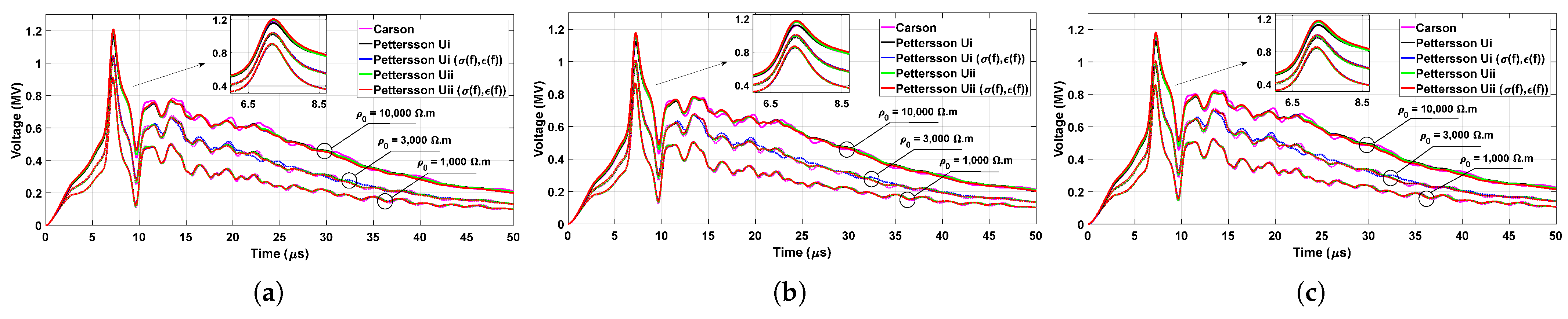
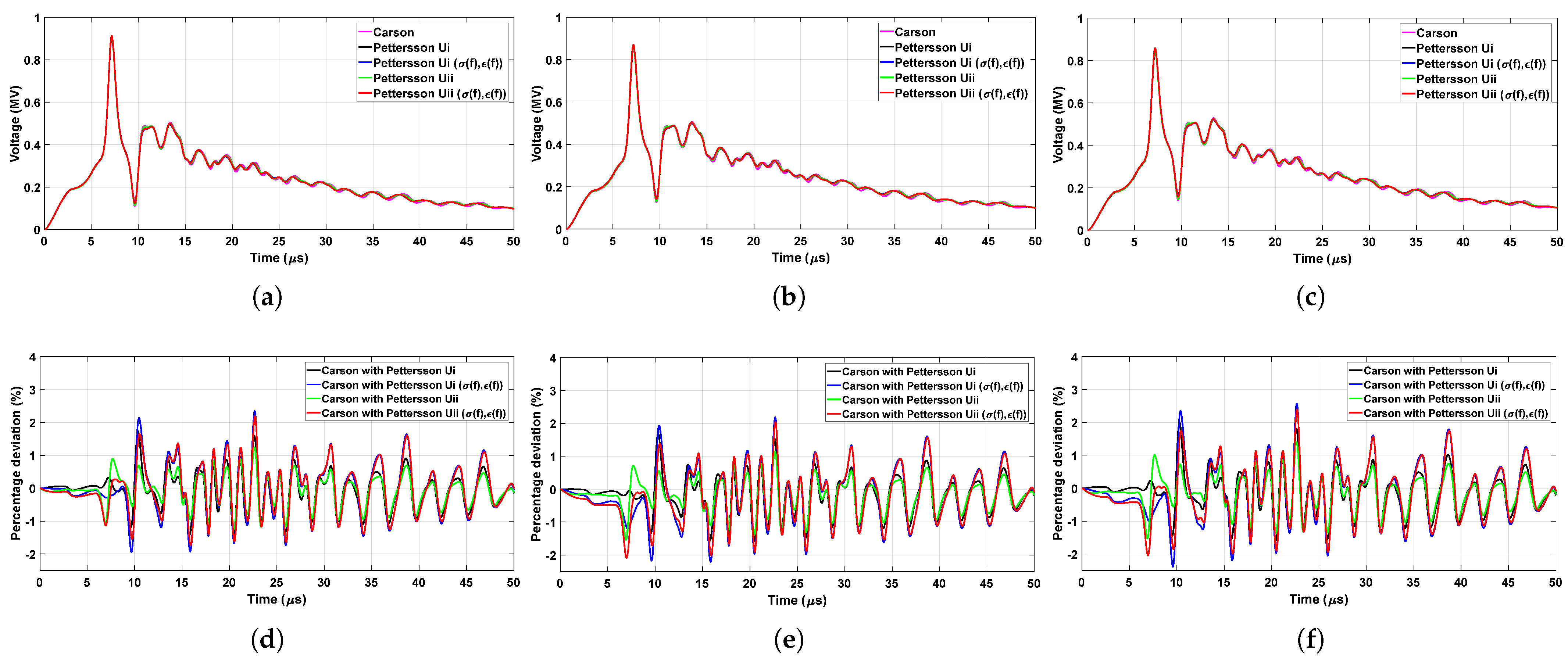
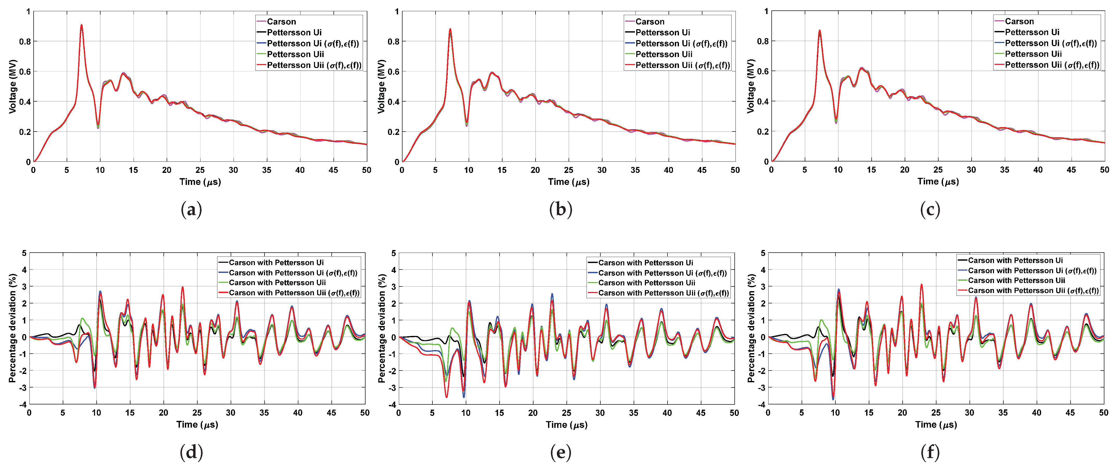
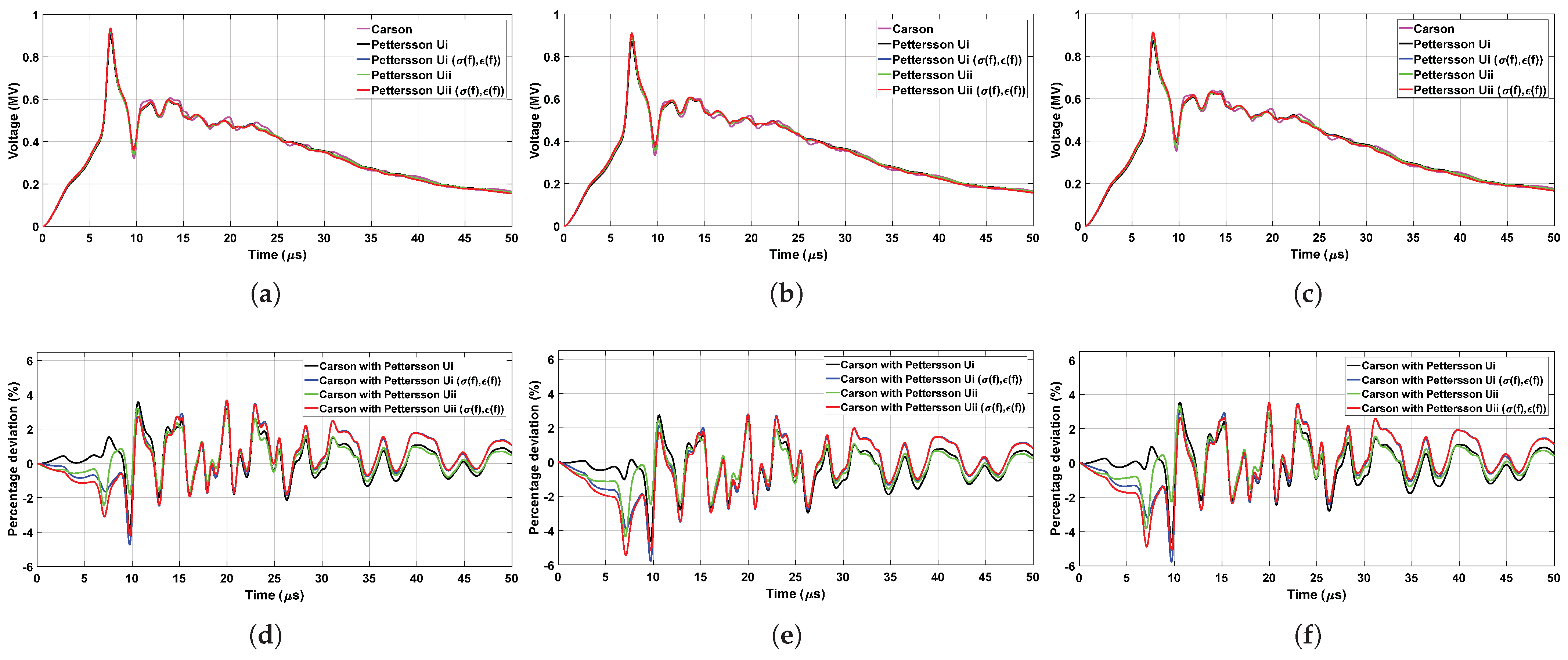
In this subsection, the overvoltage distributions in the insulator strings of phases A, B and C without the occurrence of the disruptive process are analyzed. Thus, the strings are modeled as open circuits.

4.2.1. Overvoltages

Figure 11a, Figure 11b and Figure 11c illustrate phases A, B and C lightning overvoltages, respectively, considering a lightning stroke current waveform with $\alpha$ = 1.99 parameter, the various representations of the TL shown in Table 3, and the soil resistivities of 1000 $\mathrm{\Omega }$.m, 3000 $\mathrm{\Omega }$.m and 10,000 $\mathrm{\Omega }$.m. In all figures, it can be seen that when we consider a soil with a resistivity of 1000 $\mathrm{\Omega }$.m, lightning overvoltages are smaller than when we consider a soil with a resistivity of 3000 $\mathrm{\Omega }$.m, and these are smaller than when we consider a soil with a resistivity of 10,000 $\mathrm{\Omega }$.m for all representations of the TL.

It is important to highlight that, for soils with resistivities lower than 1000 $\mathrm{\Omega }$.m, lower values of lightning overvoltages are expected, especially since these cases have lower values of grounding impedance.

4.2.2. Comparison of the Percentage Deviation of Overvoltages

The percentage deviation ($\Delta$V(%)) between the overvoltage calculated by the Pettersson formulation in relation to the reference (Carson) are shown in this subsection. The $\Delta$V(%) is computed as follows

$$\Delta V(\%)=\frac{V_{\mathrm{CA}}-V_{\mathrm{PE}}}{V_{\mathrm{CA}}}\times 100\%$$

(23)

Figure 12, Figure 13 and Figure 14 illustrate phases A, B and C lightning overvoltages (and percentage deviations), respectively, considering lightning stroke current waveforms with $\alpha$ parameter equal to 1.99, 1.66 and 1.47, respectively, (as shown in Figure 6), the various representations of the TL shown in Table 3, and the soil resistivities of 1000 $\mathrm{\Omega }$.m, 3000 $\mathrm{\Omega }$.m and 10,000 $\mathrm{\Omega }$.m.

In the case of Figure 12, it can be observed that the overvoltages in representations 2, 3, 4 and 5 present maximum percentage differences of 2.01%, 2.58%, 1.55% and 2.49%, respectively, in relation to representation 1, which is the one available in the EMT-type simulators. For Figure 13, these differences are 2.55%, 3.71%, 2.25% and 9.89%, while for Figure 14 are 4.18%, 5.93%, 4.10% and 5.82%.

According to the results, the waveforms of lightning overvoltages present the same pattern, for the Pettersson’s formulations and for the Carson’s formulation. Such behavior occurs for all ${\rho }_0$ values. Furthermore, for higher resistivities, the phase overvoltages are higher.

An interesting aspect is that the overvoltages in the insulator string of phase A are slightly higher than those of phases B and C. Since phase A is the higher one, it takes more time to notice the impact of the tower–grounding interface. It is noted for all resistivities that when considering frequency-dependent soil parameters, the percentage deviations are higher when compared to modeling via frequency-independent parameters. Furthermore, for higher resistivities, the greater the percentage deviations.

Table 4. Voltage peaks and $\Delta V_{\mathrm{peak}}$ (%) for phases A, B and C, for the ${\rho }_0$ values (1000 $\mathrm{\Omega }$.m, 3000 $\mathrm{\Omega }$.m and 10,000 $\mathrm{\Omega }$.m), and considering the 5 types of modeling representations.

	${\mathit{V}}_{\mathbf{peak}}$ (MV)			$\mathbf{\Delta }{\mathit{V}}_{\mathbf{peak}}$ (%)
	${\rho }_0$ = 1000 $\mathrm{\Omega }$.m
Rep.	A	B	C	A	B	C
1	0.905	0.855	0.845	-	-	-
2	0.907	0.855	0.843	0.232	0.070	0.225
3	0.908	0.865	0.853	0.276	1.194	0.982
4	0.910	0.866	0.855	0.497	1.385	1.195
5	0.913	0.870	0.859	0.839	1.778	1.609
	${\rho }_0$ = 3000 $\mathrm{\Omega }$.m
	A	B	C	A	B	C
1	0.899	0.853	0.853	-	-	-
2	0.894	0.854	0.849	0.556	0.152	0.399
3	0.905	0.872	0.868	0.712	2.286	1.818
4	0.908	0.876	0.870	1.023	2.368	2.052
5	0.913	0.882	0.874	1.635	3.424	2.171
	${\rho }_0$ = 10,000 $\mathrm{\Omega }$.m
	A	B	C	A	B	C
1	0.908	0.870	0.874	-	-	-
2	0.898	0.870	0.871	1.092	0.589	0.332
3	0.923	0.899	0.902	1.641	3.896	3.134
4	0.927	0.899	0.902	2.104	3.965	3.215
5	0.935	0.911	0.914	2.941	5.248	4.541

details the overvoltage peak comparisons. Moreover, according to Table 4 for more rigorous TL modeling, the percentage difference among the phases seems to increase, especially for the middle phase, i.e., phase B.

The differences reported in this subsection (both in peak values and in temporal distributions), although apparently negligible, could be decisive for the occurrence or not of the disruption process. This situation is verified in the next subsection.

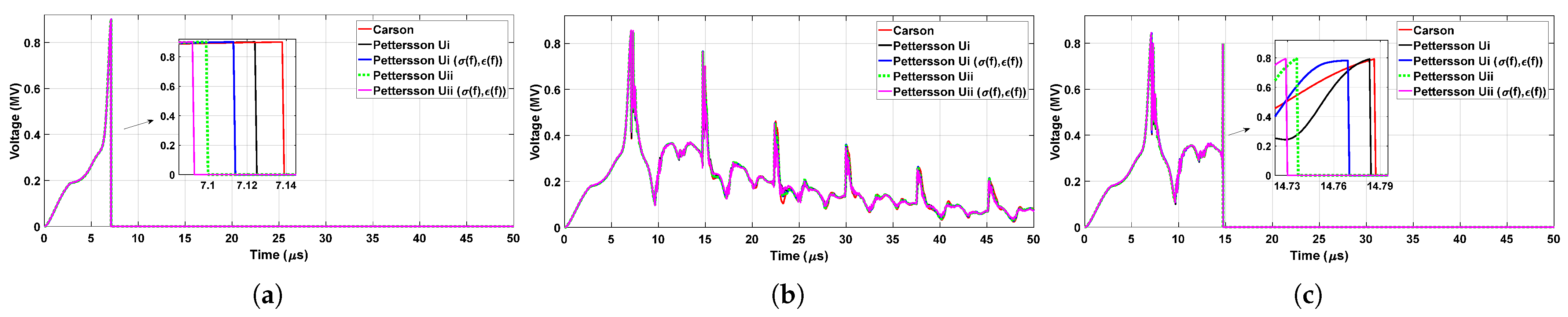
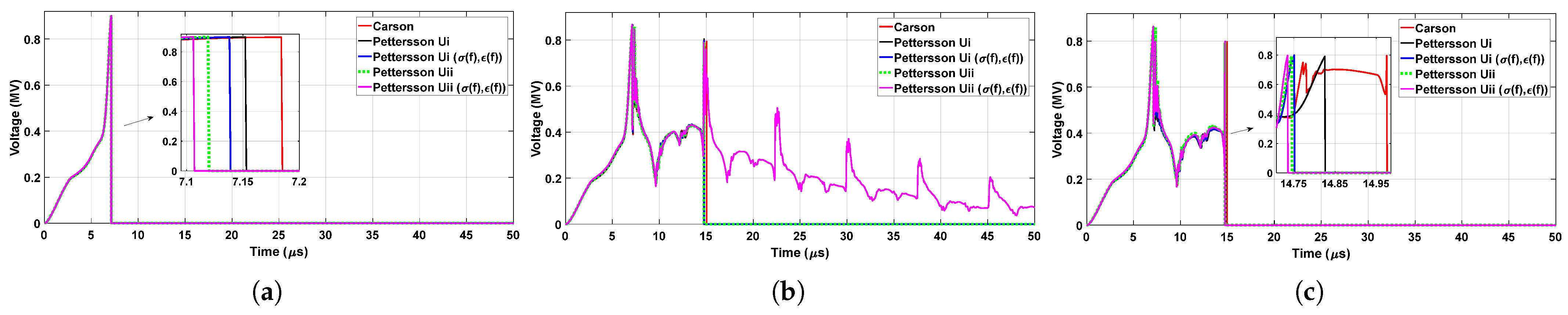
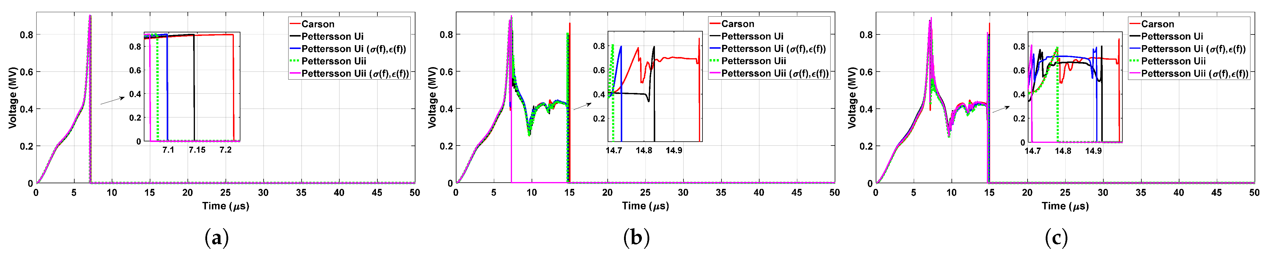
4.3. Insulator Strings Flashover

Considering the overvoltages presented in the previous subsection (Figure 12, Figure 13 and Figure 14), it is of utmost importance to verify the sensitivity of the backflashover occurrence in relation to the TL model (representations in Table 3). To accomplish this, the insulator strings are modeled using the DE method. It is important to highlight that when there is the occurrence of the disruptive effect, i.e., the insulator strings breakdown, the extremities of the insulator strings are potentially connected by an arc. In this paper, this representation is made by the usage of a TACS controlled switch. The results are illustrated in Figure 15, Figure 16 and Figure 17.

In Figure 15a, Figure 15b and Figure 15c, respectively, backflashover occurs for: (a) all line models (in approximately 7 μs); (b) no model (no occurrence) and (c) all models (in 15 μs). A similar situation occurs for the cases of soils with 3000 $\mathrm{\Omega }$.m and 10,000 $\mathrm{\Omega }$.m, Figure 16 and Figure 17, respectively. However, with different backflashover sensitivities.

Moreover, it is important to highlight that the abrupt increase in the lightning overvoltage around 15 $\mathsf{\mu }$s, which can be seen in Figure 15b,c, Figure 16b,c and Figure 17b,c, occurs due to the insulator breakdown in phase A.

Table 5. Sensitivity of backflashover occurrence as a function of the transmission line model.

${\mathit{\rho }}_0$ (Ω.m)	Backflashover Occurrence
	Insulator String in Phase	Types of Modeling Representations (Table 3)	Disruption Time ($\mathsf{\mu }$s)
	A	1, 2, 3, 4 and 5	7
1000	B	-	-
	C	1, 2, 3, 4 and 5	15
	A	1, 2, 3, 4 and 5	7
3000	B	1, 2, 3 and 4	15
	C	1, 2, 3, 4 and 5	15
	A	1, 2, 3, 4 and 5	7
10,000	B	5	7
		1, 2, 3 and 4	15
	C	1, 2, 3, 4 and 5	15

summarizes the backflashover occurrences, as well as the time when the disruption occurs. These results illustrate the significant importance that the line model has on the string insulator disruption process. The strings of phases A and C always break in 7 $\mathsf{\mu }$s and 15 $\mathsf{\mu }$s, respectively, while those of phase B in both instants. The types of modeling representations in which disruptions occur vary with phase and soil resistivity. Some electromagnetic transients software, such as the ATP, use representation 1 to model transmission lines. However, according to the results of Table 5, in phase B, for example, for 3000 $\mathrm{\Omega }$.m the backflashover phenomenon does not occur for representation 5 and for 10,000 $\mathrm{\Omega }$.m soils the backflashover occurs only for representation 5 (at 7 $\mathsf{\mu }$s), i.e., using simplified methodologies may result in misleading lightning performance estimations.

5. Conclusions

This paper has presented sensitivity analyses of TL parameters (longitudinal and transversal) and lightning overvoltages in insulator strings considering the Pettersson formulation (more physically consistent) of the transmission line, which consider the displacement current, ground admittance correction, rigorous voltage definition and frequency-dependent soil parameters. For this analysis, five different formulations were compared to compute the soil effect in the TL parameters, as illustrated in Table 5 of the paper. Moreover, for the analysis, the TL represented by the J. Marti model, with the ground effect included through J. R. Carson’s formulation (less physically consistent), was used as a reference, because this representation of the TL is the only one available in the ATP software. The results obtained (using a typical TL of 138 kV as a case) illustrate that, considering J. R. Carson as a reference:

• The longitudinal parameters (resistance $R$ and inductance $L$) are very sensitive to the model considered, especially from 1 kHz. In the frequency range of the first return strokes, the maximum percentage differences for $R$ and $L$ (both self and mutual) were, respectively, 71.54% and 34.66%. The transversal parameter ($C$ capacitance) is practically insensitive, with a maximum difference equal to 3.61%.
• The occurrence or not of backflashover in the insulator strings, including the disruption time, are also sensitive to the formulation considered and the line location above soil (good or poorly conductor). For the case of 1000 $\mathrm{\Omega }$.m, it was found that there were no major differences for the five formulations of the TL. For the case of 3000 $\mathrm{\Omega }$.m, it was found that in phase B, the only one of the five formulations that did not backflashover was the Pettersson formulation (more physically consistent). For the case of 10,000 $\mathrm{\Omega }$.m, it was observed that the only difference, in the five formulations, was in the rupture time that occurred for the Pettersson formulation (more physically consistent). Emphasis is given to phase B whose height is intermediate between those of phases A (highest) and C (lowest), as illustrated in the Table 5 of the paper. This sensitivity, to the best of the authors’ knowledge, is not reported in the available technical literature.

We hope the results presented in this paper will motivate the implementation of the Pettersson formulation (more physically consistent) in the main EMT-type simulators. For future work, the extension of the analyses carried out for transmission lines of other voltage levels, new analyses for the incidence of lightning strikes in the midspan of the transmission line, the shutdown rate due to backflashover of the transmission line will be studied, and analyses with the inclusion of non-linear elements and/or effects that vary over time, such as lightning rods made from emerging technologies [40].

References

1. Visacro, S.; Soares, A. HEM: A model for simulation of lightning-related engineering problems. IEEE Trans. Power Deliv. 2005, 20, 1206–1208. [Google Scholar] [CrossRef]
2. Schroeder, M.A.O.; Correia de Barros, M.T.; Lima, A.C.S.; Afonso, M.M.; Moura, R.A.R. Evaluation of the impact of different frequency dependent soil models on lightning overvoltages. Electr. Power Syst. Res. 2018, 159, 40–49. [Google Scholar] [CrossRef]
3. Batista, R.; Louro, P.E.; Paulino, J.O. Lightning performance of a critical path from a 230-kV transmission line with grounding composed by deep vertical electrodes. Electr. Power Syst. Res. 2021, 195, 107165. [Google Scholar] [CrossRef]
4. Gomes, T.V.; Schroeder, M.A.O.; Alipio, R.; de Lima, A.C.S.; Piantini, A. Investigation of Overvoltages in HV Underground Sections Caused by Direct Strokes Considering the Frequency-Dependent Characteristics of Grounding. IEEE Trans. Electromagn. Compat. 2018, 60, 2002–2010. [Google Scholar] [CrossRef]
5. Banjanin, M.S. Application possibilities of special lightning protection systems of overhead distribution and transmission lines. Int. J. Electr. Power Energy Syst. 2018, 100, 482–488. [Google Scholar] [CrossRef]
6. Papadopoulos, T.A.; Chrysochos, A.I.; Traianos, C.K.; Papagiannis, G. Closed-Form Expressions for the Analysis of Wave Propagation in Overhead Distribution Lines. Energies 2020, 13, 4519. [Google Scholar] [CrossRef]
7. Longmire, C.L.; Smith, K.S. A Universal Impedance for Soils; Technical Report; Mission Research Corp: Santa Barbara, CA, USA, 1975.
8. CIGRE Working Group C4.33. Impact of Soil-Parameter Frequency Dependence on the Response of Grounding Electrodes and on the Lightning Performance of Electrical Systems. Technical Brochure 781. 2019, pp. 1–66. Available online: https://e-cigre.org/publication/781-impactof-soil-parameter-frequency-dependence-on-the-response-of-grounding-electrodes-and-on-the-lightning-performance-ofelectrical-systems (accessed on 16 September 2022).
9. Lima, A.C.S.; Moura, R.A.R.; Schroeder, M.A.O.; Correia de Barros, M.T. Assessment of different formulations for the ground return parameters in modeling overhead lines. Electr. Power Syst. Res. 2018, 164, 20–30. [Google Scholar] [CrossRef]
10. Diniz, F.A.; Alípio, R.S.; Moura, R.A.R. Assessment of the Influence of Ground Admittance Correction and Frequency Dependence of Electrical Parameters of Ground of Simulation of Electromagnetic Transients in Overhead Lines. J. Control. Autom. Electr. Syst. 2022, 33, 1066–1080. [Google Scholar] [CrossRef]
11. De Conti, A.; Emídio, M.P.S. Extension of a modal-domain transmission line model to include frequency-dependent ground parameters. Electr. Power Syst. Res. 2016, 138, 120–130. [Google Scholar] [CrossRef]
12. Colqui, J.S.L.; Araújo, A.R.J.D.; Pascoalato, T.F.G.; Kurokawa, S.; Filho, J.P. Transient Analysis on Multiphase Transmission Line Above Lossy Ground Combining Vector Fitting Technique in ATP Tool. IEEE Access 2022, 10, 86204–86214. [Google Scholar] [CrossRef]
13. Alípio, R.S.; De Conti, A.; Miranda, A.; Correia de Barros, M.T. Lightning Overvoltages Including Frequency-Dependent Soil Parameters in the Transmission Line Model. In Proceedings of the International Conference on Power Systems Transients (IPST), Perpignan, France, 16–20 June 2019. [Google Scholar]
14. Pettersson, P. Propagation of waves on a wire above a lossy ground-different formulations with approximations. IEEE Trans. Power Deliv. 1999, 14, 1173–1180. [Google Scholar] [CrossRef]
15. Tomasevich, M.M.Y.; Lima, A.C.S. Impact of Frequency-Dependent Soil Parameters in the Numerical Stability of Image Approximation-Based Line Models. IEEE Trans. Electromagn. Compat. 2016, 58, 323–326. [Google Scholar] [CrossRef]
16. Magalhães, A.P.C.; Silva, J.C.L.V.; Lima, A.C.; Correia De Barros, M.T. Validation Limits of Quasi-TEM Approximation for Buried Bare and Insulated Cables. IEEE Trans. Electromagn. Compat. 2015, 57, 1690–1697. [Google Scholar] [CrossRef]
17. Tomasevich, M.M.Y.; Lima, A.C.S. Investigation on the limitation of closed-form expressions for wideband modeling of overhead transmission lines. Electr. Power Syst. Res. 2016, 130, 113–123. [Google Scholar] [CrossRef]
18. Nakagawa, M. Admittance Correction Effects of a Single Overhead Line. IEEE Trans. Power Appar. Syst. 1981, PAS-100, 1154–1161. [Google Scholar] [CrossRef]
19. Carson, J.R. Wave Propagation in Overhead Wires with Ground Return. Bell Syst. Tech. J. 1926, 5, 539–554. [Google Scholar] [CrossRef]
20. Sunde, E.D. Earth Conduction Effects in Transmission Systems; Dover Publications: New York, NY, USA, 1968; p. 383. [Google Scholar] [CrossRef]
21. Lima, G.S.; De Conti, A. Bottom-up single-wire power line communication channel modeling considering dispersive soil characteristics. Electr. Power Syst. Res. 2018, 165, 35–44. [Google Scholar] [CrossRef]
22. Marti, J.R. Accurate Modeling of Frequency-Dependent Transmission Lines in Electromagnetic Transient Simulations. IEEE Power Eng. Rev. 1982, 2, 29–30. [Google Scholar] [CrossRef]
23. Dommel, H.W. EMTP Theory Book; Microtran Power System Analysis Corporation: Vancouver, BC, Canada, 1996. [Google Scholar]
24. Gustavsen, B.; Semlyen, A. Rational approximation of frequency domain responses by vector fitting. IEEE Trans. Power Deliv. 1999, 14, 1052–1061. [Google Scholar] [CrossRef] [Green Version]
25. Cabral, E.S.B.; Robles, J.A.G.; Sánchez, J.L.G.; Castañón, J.S.; Sánchez, V.A.G. Accuracy enhancement of the JMarti model by using real poles through vector fitting. Electr. Eng. 2019, 101, 635–646. [Google Scholar] [CrossRef]
26. Cavka, D.; Mora, N.; Rachidi, F. A Comparison of frequency-dependent soil models: Application to the analysis of grounding systems. IEEE Trans. Electromagn. Compat. 2014, 56, 177–187. [Google Scholar] [CrossRef]
27. Alípio, R.S.; Visacro, S. Modeling the frequency dependence of electrical parameters of soil. IEEE Trans. Electromagn. Compat. 2014, 56, 1163–1171. [Google Scholar] [CrossRef]
28. Piantini, A. Lightning Interaction with Power Systems—Volume 1: Fundamentals and Modelling; Institution of Engineering and Technology: London, UK, 2020; p. 456. [Google Scholar] [CrossRef]
29. De Conti, A.; Visacro, S.; Soares, A.; Schroeder, M.A.O. Revision, extension, and validation of Jordan’s formula to calculate the surge impedance of vertical conductors. IEEE Trans. Electromagn. Compat. 2006, 48, 530–536. [Google Scholar] [CrossRef]
30. Imece, A.F.; Durbak, D.W.; Elahi, H.; Kolluri, S.; Lux, A.; Mader, D.; McDermott, T.E.; Morched, A.; Mousa, A.M.; Natarajan, R.; et al. Modeling guidelines for fast front transients. IEEE Trans. Power Deliv. 1996, 11, 493–501. [Google Scholar] [CrossRef]
31. Witzke, R.L.; Bliss, T.J. Co-ordination of Lightning Arrester Location with Transformer Insulation Level. Trans. Am. Inst. Electr. Eng. 1950, 69, 964–975. [Google Scholar] [CrossRef]
32. Pigini, A.; Rizzi, G.; Garbagnati, E.; Porrino, A.; Baldo, G.; Pesavento, G. Performance of large air gaps under lightning overvoltages: Experimental study and analysis of accuracy predetermination methods. IEEE Trans. Power Deliv. 1989, 4, 1379–1392. [Google Scholar] [CrossRef]
33. Banjanin, M.S.; Savić, M.S. Some aspects of overhead transmission lines lightning performance estimation in engineering practice. Int. Trans. Electr. Energy Syst. 2016, 26, 79–93. [Google Scholar] [CrossRef]
34. Visacro, S.; Silveira, F.H. Lightning Performance of Transmission Lines: Methodology to Design Grounding Electrodes to Ensure an Expected Outage Rate. IEEE Trans. Power Deliv. 2015, 30, 237–245. [Google Scholar] [CrossRef]
35. Visacro, S.; Soares, A., Jr.; Schroeder, M.A.O.; Cherchiglia, L.C.; de Sousa, V.J. Statistical analysis of lightning current parameters: Measurements at Morro do Cachimbo Station. J. Geophys. Res. 2004, 109, 1–11. [Google Scholar] [CrossRef]
36. De Conti, A.; Visacro, S. Analytical representation of single- and double-peaked lightning current waveforms. IEEE Trans. Electromagn. Compat. 2007, 49, 448–451. [Google Scholar] [CrossRef]
37. CIGRE Working Group C4.23. Procedures for Estimating the Lightning Performance of Transmission Lines – New Aspects. Technical Brochure 839. 2021, pp. 1–66. Available online: https://e-cigre.org/publication/063-guide-to-procedures-for-estimating-the-lightning-performance-of-transmission-lines (accessed on 16 September 2022).
38. Oliveira, A.J.; Schroeder, M.A.O.; Moura, R.A.; De Barros, M.T.C.; Lima, A.C. Adjustment of current waveform parameters for first lightning strokes: Representation by Heidler functions. In Proceedings of the 2017 International Symposium on Lightning Protection, XIV SIPDA, Natal, Brazil, 2–6 October 2017; pp. 121–126. [Google Scholar]
39. Pascoalato, T.F.G.; de Araújo, A.R.J.; Caballero, P.T.; Colqui, J.S.L.; Kurokawa, S. Transient Analysis of Multiphase Transmission Lines Located above Frequency-Dependent Soils. Energies 2021, 14, 5252. [Google Scholar] [CrossRef]
40. Xu, H.; Cao, G.; Shen, Y.; Yu, Y.; Hu, J.; Wang, Z.; Shao, G. Enabling Argyrodite Sulfides as Superb Solid-State Electrolyte with Remarkable Interfacial Stability Against Electrodes. Energy Environ. Mater. 2022, 5, 852–864. [Google Scholar] [CrossRef]
Figure 1. Configuration of the conductors for an overhead line.
Energies 16 01343 g001
Figure 2. Diagram of the strategy used in the implementation of modified J. Marti model in ATP.
Energies 16 01343 g002
Figure 3. (a) Tower silhouette and; (b) Arrangement of tower-footing grounding electrodes.
Energies 16 01343 g003
Figure 4. Schematic representation of the transmission tower [2].
Energies 16 01343 g004
Figure 5. Magnitude of the harmonic grounding impedance.
Energies 16 01343 g005
Figure 6. Simulated first stroke current waveforms considering different values of current peak.
Energies 16 01343 g006
Figure 7. System transmission implementation in ATP.
Energies 16 01343 g007
Figure 8. (a) Resistance ( Ω /km) for the 1000 Ω .m; (b) Resistance ( Ω /km) for the 10,000 Ω .m; (c) Percentage deviation between Carson’s and Pettersson’s formulation Ui; (d) Percentage deviation between Carson’s and Pettersson’s formulation Ui with frequency dependence; (e) Percentage deviation between Carson’s and Pettersson’s formulation Uii; (f) Percentage deviation between Carson’s and Pettersson’s formulation Uii with frequency dependence.
Energies 16 01343 g008
Figure 9. (a) Inductance (mH/km) for the 1000 Ω .m; (b) Inductance (mH/km) for the 10,000 Ω .m; (c) Percentage deviation between Carson’s and Pettersson’s formulation Ui; (d) Percentage deviation between Carson’s and Pettersson’s formulation Ui with frequency dependence; (e) Percentage deviation between Carson’s and Pettersson’s formulation Uii; (f) Percentage deviation between Carson’s and Pettersson’s formulation Uii with frequency dependence.
Energies 16 01343 g009
Figure 10. (a) Capacitance ( μ F/km) for the 1000 Ω .m; (b) Capacitance ( μ F/km) for the 10,000 Ω .m; (c) Percentage deviation between Carson’s and Pettersson’s formulation Ui; (d) Percentage deviation between Carson’s e Pettersson’s formulation Ui with frequency dependence; (e) Percentage deviation between Carson’s and Pettersson’s formulation Uii; (f) Percentage deviation between Carson’s and Pettersson’s formulation Uii with frequency dependence.
Energies 16 01343 g010
Figure 11. Overvoltage waveforms in phases A (a), B (b) and C (c), with or without a disruption process (backflashover), considering a lightning stroke current waveform with α = 1.99, and ground resistivities equal to 1000 Ω .m, 3000 Ω .m and 10,000 Ω .m.
Energies 16 01343 g011
Figure 12. Overvoltage waveforms in phases A (a), B (b) and C (c) and percentage differences, based on Carson’s formulation, for phases A (d), B (e) and C (f), considering ground resistivity equal to 1000 Ω .m and a lightning stroke current waveform with α = 1.99.
Energies 16 01343 g012
Figure 13. Overvoltage waveform in phases A (a), B (b) and C (c) and percentage differences, based on Carson’s formulation, for phases A (d), B (e) and C (f), considering ground resistivity equal to 3000 Ω .m and a lightning stroke current waveform with α = 1.66.
Energies 16 01343 g013
Figure 14. Overvoltage waveform in phases A (a), B (b) and C (c) and percentage differences, based on Carson’s formulation, for phases A (d), B (e) and C (f), considering ground resistivity equal to 10,000 Ω .m and a lightning stroke current waveform with α = 1.47.
Energies 16 01343 g014
Figure 15. Overvoltage waveforms in phases A (a), B (b) and C (c), with or without a disruption process (backflashover), considering ground resistivity equal to 1000 Ω .m and a lightning stroke current waveform with α = 1.99.
Energies 16 01343 g015
Figure 16. Overvoltage waveforms in phases A (a), B (b) and C (c), with or without a disruption process (backflashover), considering ground resistivity equal to 3000 Ω .m and a lightning stroke current waveform with α = 1.66.
Energies 16 01343 g016
Figure 17. Overvoltage waveforms in phases A (a), B (b) and C (c), with or without a disruption process (backflashover), considering ground resistivity equal to 10,000 Ω .m. and a lightning stroke current waveform with α = 1.47.
Energies 16 01343 g017