


Influence of PPD and Mass Scaling Parameter on the Goodness of Fit of Dry Ice Compaction Curve Obtained in Numerical Simulations Utilizing Smoothed Particle Method (SPH) for Improving the Energy Efficiency of Dry Ice Compaction Process


Abstract
:1. Introduction
2. Materials and Methods
2.1. Materials
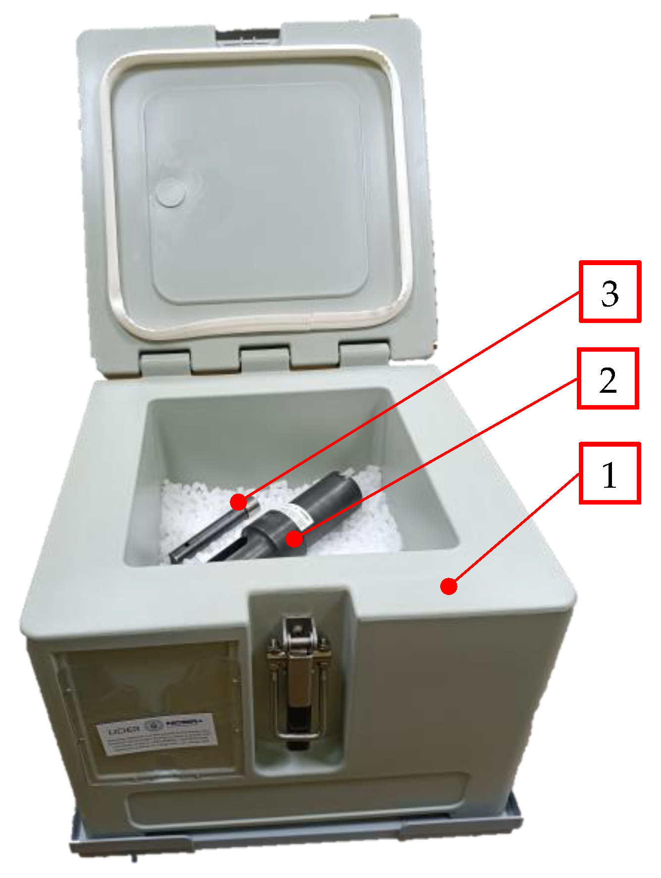
2.1.1. Powder
2.1.2. Compaction
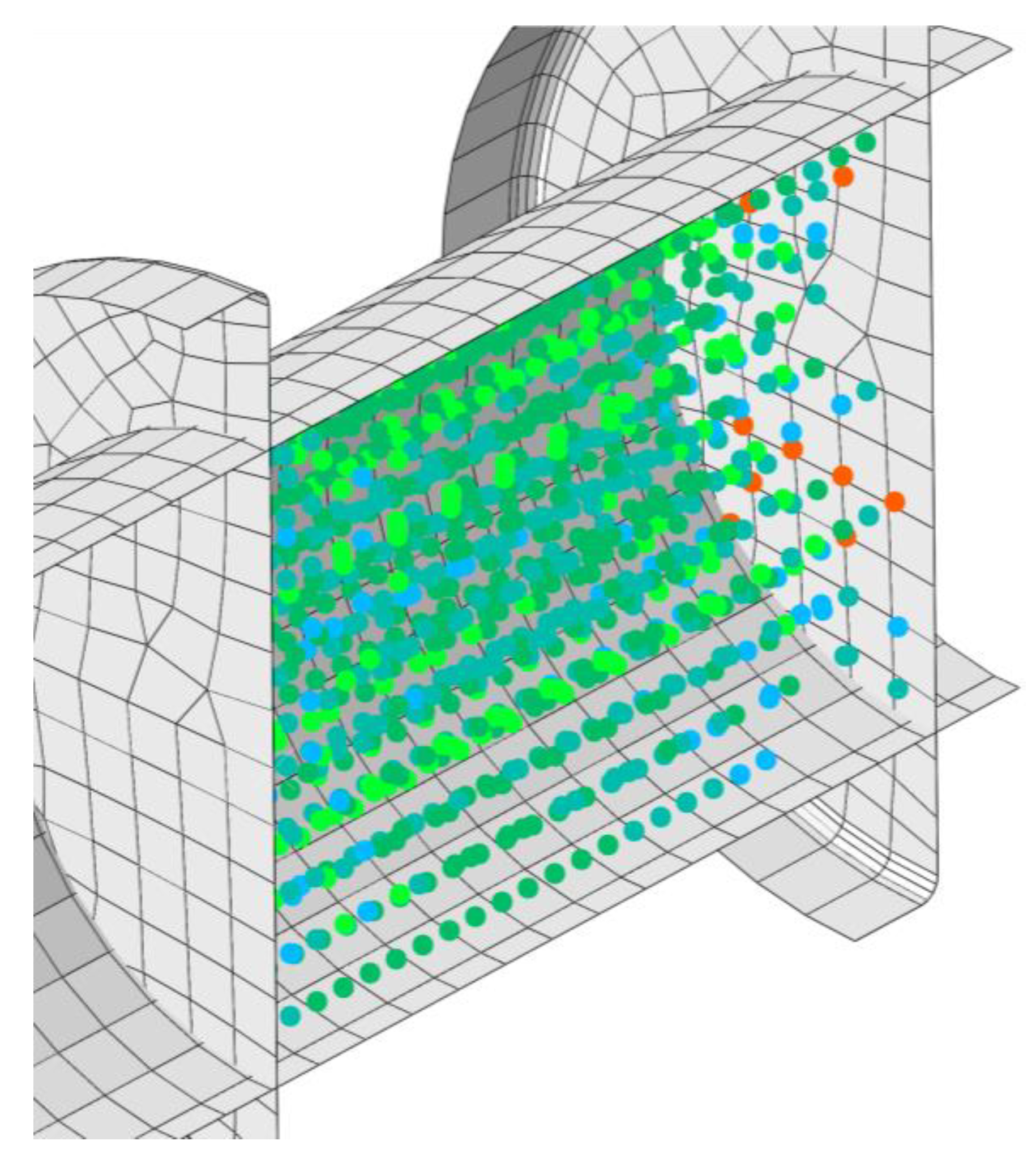
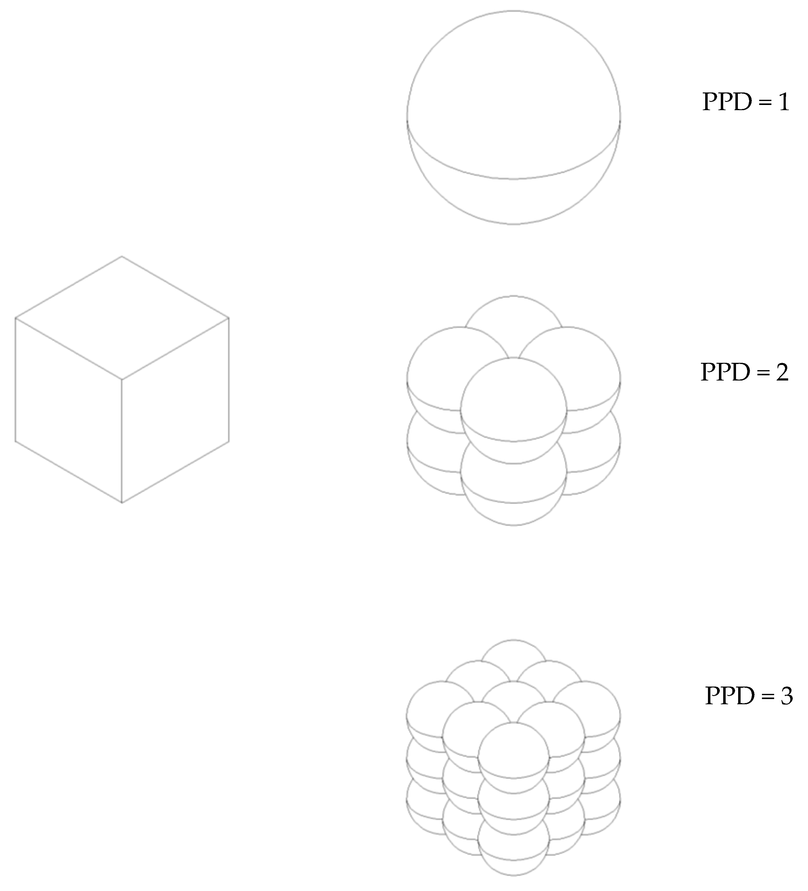
2.2. Numerical Model
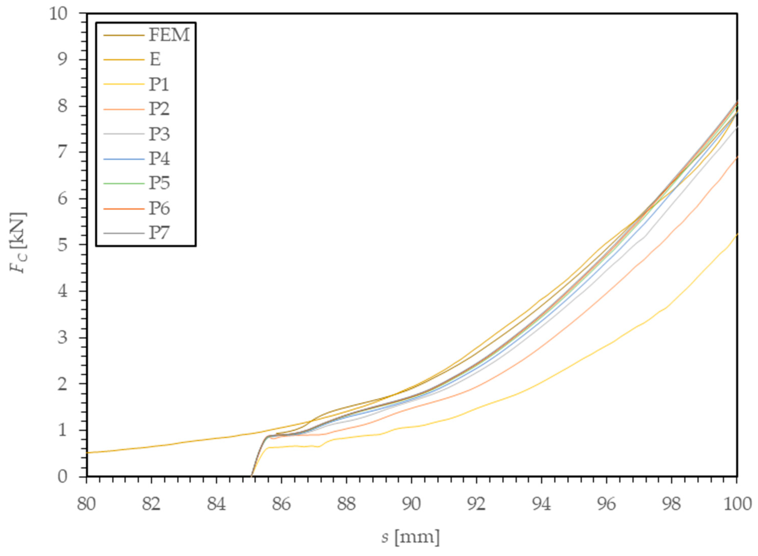
3. Results and Discussion
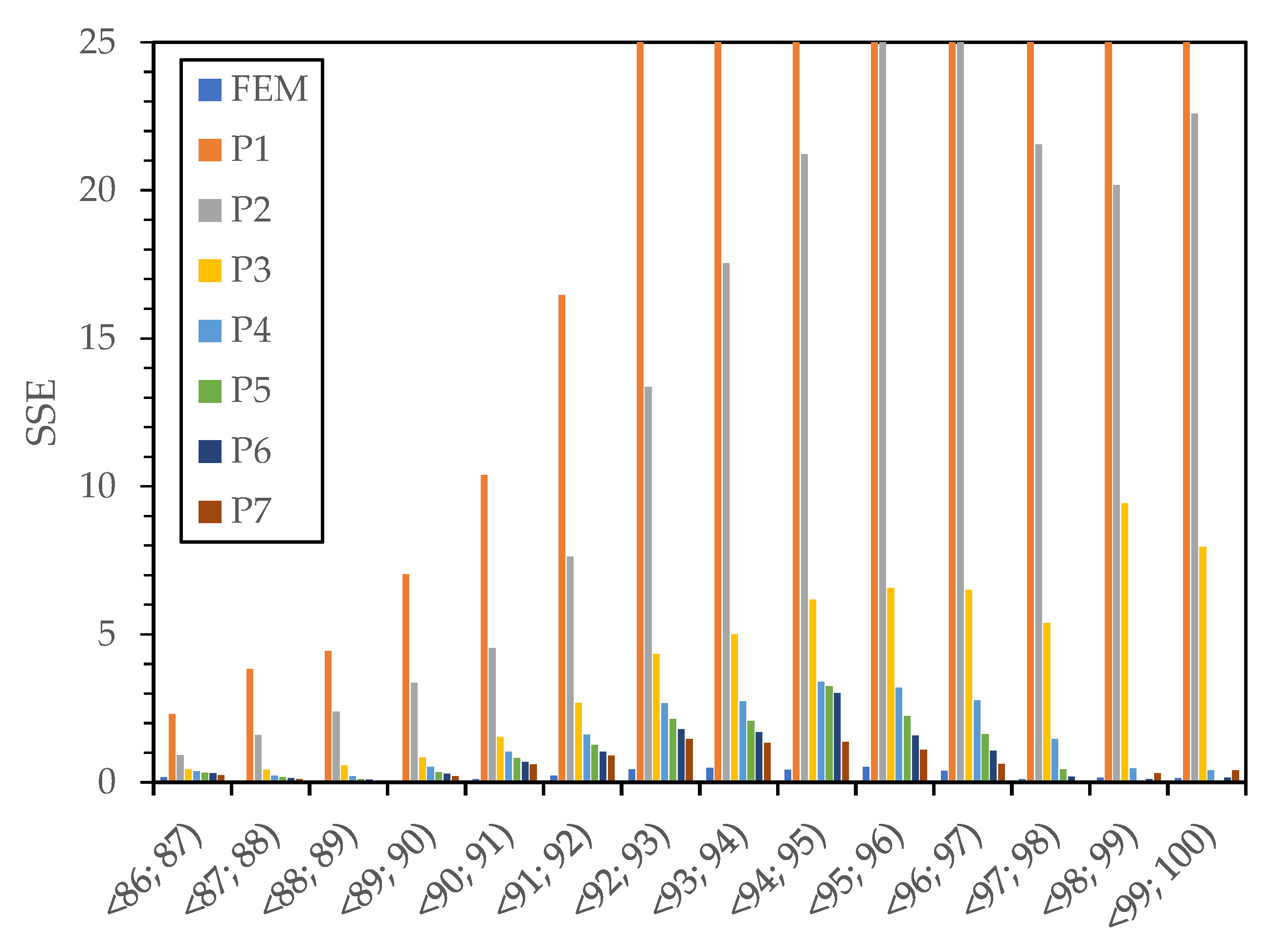
- The greater the PPD value, the better the fit obtained between the simulation and experimental curves.
- An increase in PPD reduces the difference between the calculated and experimental ultimate force values.
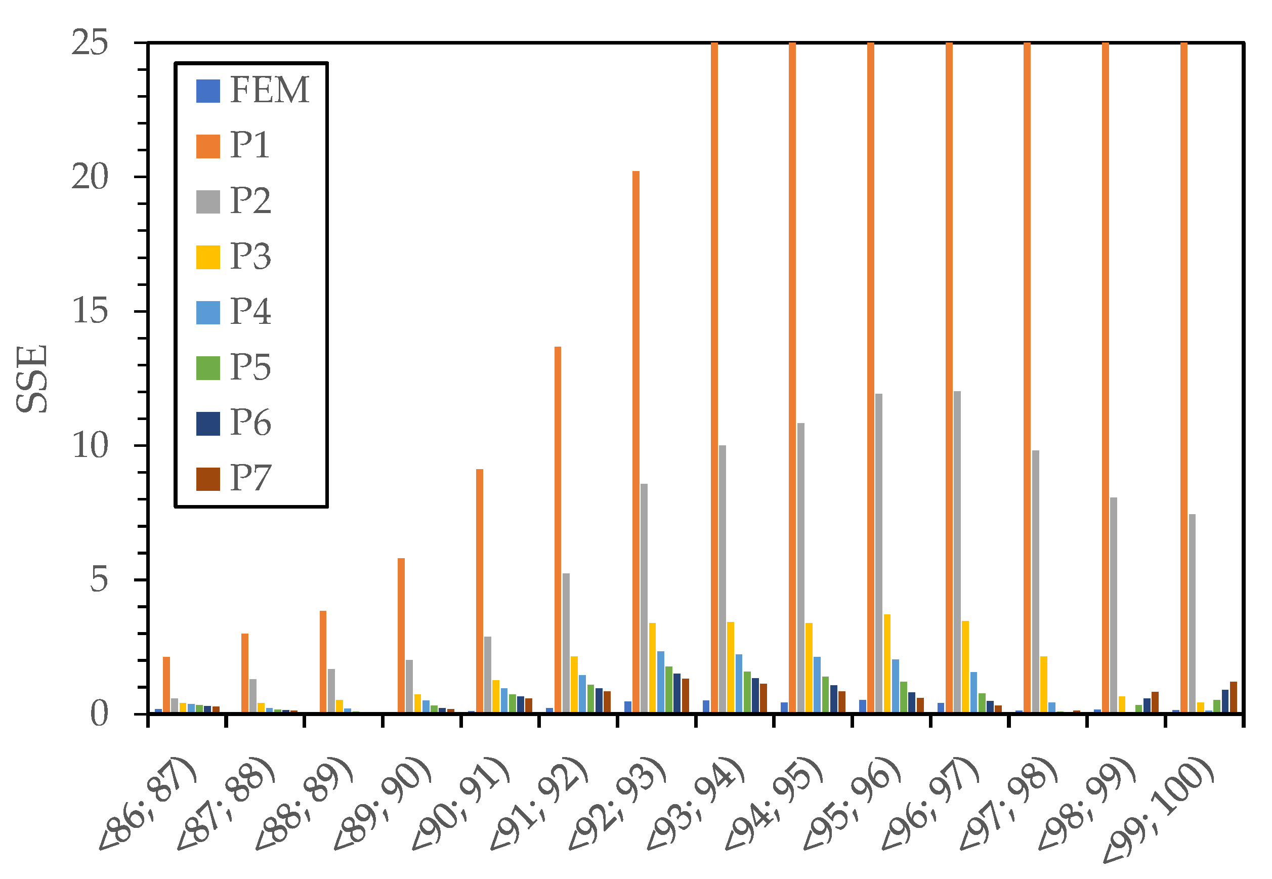
- The greater the MS value, the better the fit obtained between the simulation and experimental curves.
- An increase in MS reduces the difference between the calculated and experimental ultimate force values.
- FS—value of FC obtained in numerical simulation;
- FE—experimental FC value used as reference.
4. Conclusions
Author Contributions
Funding
Data Availability Statement
Conflicts of Interest
References
- Gierz, Ł.; Warguła, Ł.; Kukla, M.; Koszela, K.; Zawiachel, T. Computer Aided Modeling of Wood Chips Transport by Means of a Belt Conveyor with Use of Discrete Element Method. Appl. Sci. 2020, 10, 9091. [Google Scholar] [CrossRef]
- Omer, O.; Alireza, K. Alternative Energy in Power Electronics: Chapter 2 Energy in Power Electronics; Butterworth-Heinemann: Oxford, UK, 2015; pp. 81–154. [Google Scholar] [CrossRef]
- Tahmasebi, M.M.; Banihashemi, S.; Hassanabadi, M.S. Assesment of the Variation Impacts og Windwos on Energy Consumption and Carbon Footprint. Procedua Eng. 2011, 21, 820–828. [Google Scholar] [CrossRef]
- Lohri, C.; Rajabu, H.; Sweeney, D.; Zurbrügg, C. Char fuel production in developing countries—A review of urban biowaste carbonization. Renew. Sustain. Energy Rev. 2016, 59, 1514–1530. [Google Scholar] [CrossRef]
- Gawrońska, E.; Dyja, R. A Numerical Study of Geometry’s Impact on the Thermal and Mechanical Properties of Periodic Surface Structures. Appl. Sci. 2021, 14, 427. [Google Scholar] [CrossRef] [PubMed]
- Wilczyński, D.; Talaśka, K.; Wojtokwiak, D.; Wałęsa, K.; Wojciechowski, S. Selection of the Electric Drive for the Wood Waste Compacting Unit. Energies 2022, 15, 7488. [Google Scholar] [CrossRef]
- Ishiguro, M.; Dan, K.; Nakasora, K.; Morino, Y.; Yoshii, Y.; Chaki, T. Increase of Snow Compaction Density by Repeated Articial Snow Consolidation Formation. J. Inst. Ind. Appl. Eng. 2020, 8, 104. [Google Scholar] [CrossRef]
- Baiul, K.; Vashchenko, S.; Khudyakov, O.; Bembenek, M.; Zinchenko, A.; Krot, P.V.; Solodka, N. A Novel Approach to the Screw Feeder Design to Improve the Reliability of Briquetting Process in the Roller Press. Eksploat. Niezawodn.—Maint. Reliab. 2023, 25, 167967. [Google Scholar] [CrossRef]
- Warguła, Ł.; Wojtkowiak, D.; Kukla, M.; Talaśka, K. Modelling the process of splitting wood and chipless cutting Pinus sylvestris L. wood in terms of designing the geometry of the tools and the driving force of the machine. Eur. J. Wood Wood Prod. 2022, 81, 223–237. [Google Scholar] [CrossRef]
- Gierz, Ł.; Kolankowska, E.; Markowski, P.; Koszela, K. Measurements and Analysis of the Physical Properties of Cereal Seeds Depending on Their Moisture Content to Improve the Accuracy of DEM Simulation. Appl. Sci. 2022, 12, 549. [Google Scholar] [CrossRef]
- Lin, L.; Zeheng, G.; Weixin, X.; Yunfeng, T.; Xinghua, F.; Dapeng, T. Mixing mass transfer mechanism and dynamic control of gas-liquid-solid multiphase flow based on VOF-DEM coupling. Energy 2023, 272, 127015. [Google Scholar] [CrossRef]
- Ge, M.; Chen, J.; Zhao, L.; Zheng, G. Mixing Transport Mechanism of Three-Phase Particle Flow Based on CFD-DEM Coupling. Processes 2023, 11, 1619. [Google Scholar] [CrossRef]
- Giannis, K.; Schilde, C.; Finke, J.H.; Kwade, A. Modeling of High-Density Compaction of Pharmaceutical Tablets Using Multi-Contact Discrete Element Method. Pharmaceutics 2021, 13, 2194. [Google Scholar] [CrossRef]
- Harthong, B.; Jérier, J.-F.; Dorémus, P.; Imbault, D.; Donzé, F.V. Modeling of high-density compaction of granular materials by the Discrete Element Method. Int. J. Solids Struct. 2009, 46, 3357–3364. [Google Scholar] [CrossRef]
- Wu, Z.; Yu, F.; Zhang, P.; Liu, X. Micro-mechanism study on rock breaking behavior under water jet impact using coupled SPH-FEM/DEM method with Voronoi grains. Eng. Anal. Bound. Elem. 2019, 108, 472–483. [Google Scholar] [CrossRef]
- Jagota, V.; Sethi, A.P.; Kumar, K. Finite Element Method: An Overview. Walailak J. Sci. Technol. 2013, 10, 1–8. Available online: https://wjst.wu.ac.th/index.php/wjst/article/view/499 (accessed on 6 July 2023).
- Wang, W.; Wu, Y.; Wu, H.; Yang, C.; Feng, Q. Numerical analysis of dynamic compaction using FEM-SPH coupling method. Soil Dyn. Earthq. Eng. 2021, 140, 106420. [Google Scholar] [CrossRef]
- Yagawa, G.; Furukawa, T. Recent development of free mesh method. Int. J. Numer. Meth. Eng. 2000, 47, 1419–1443. [Google Scholar]
- Bahrami, M.; Naderi-Boldaji, M.; Ghanbarian, D.; Keller, T. Simulation of soil stress under plate sinkage loading: A comparison of finite element and discrete element methods. Soil Tillage Res. 2022, 223, 105463. [Google Scholar] [CrossRef]
- Gierz, Ł.; Kruszelnicka, W.; Robakowska, M.; Przybył, K.; Koszela, K.; Marciniak, A.; Zwiachel, T. Optimization of the Sowing Unit of a Piezoelectrical Sensor Chamber with the Use of Grain Motion Modeling by Means of the Discrete Element Method. Case Study: Rape Seed. Appl. Sci. 2022, 12, 1594. [Google Scholar] [CrossRef]
- Libersky, L.; Perschek, A.; Carney, T.; Hipp, C.; Allahdadi, F. High Strain Lagrangian Hydrodynamics: A Three-Dimensional SPH Code for Dynamic Material Response. J. Comput. Phys. 1993, 109, 67–75. [Google Scholar] [CrossRef]
- Berdychowski, M.; Górecki, J.; Biszczanik, A.; Wałęsa, K. Numerical Simulation of Dry Ice Compaction Process: Comparison of Drucker-Prager/Cap and Cam Clay Models with Experimental Results. Materials 2022, 15, 5771. [Google Scholar] [CrossRef] [PubMed]
- Berdychowski, M.; Górecki, J.; Wałęsa, K. Numerical Simulation of Dry Ice Compaction Process: Comparison of the Mohr–Coulomb Model with the Experimental Results. Materials 2022, 15, 7932. [Google Scholar] [CrossRef] [PubMed]
- Wałęsa, K.; Górecki, J.; Berdychowski, M.; Biszczanik, A.; Wojtkowiak, D. Modelling of the Process of Extrusion of Dry Ice through a Single-Hole Die Using the Smoothed Particle Hydrodynamics (SPH) Method. Materials 2022, 15, 8242. [Google Scholar] [CrossRef] [PubMed]
- Jankowiak, T.; Łodygowski, T. Using of Smoothed Particle Hydrodynamics (SPH) method for concrete application. Bull. Pol. Acad. Sci. Tech. Sci. 2013, 61, 111–121. [Google Scholar] [CrossRef]
- Górecki, J.; Wiktor, Ł. Influence of Die Land Length on the Maximum Extrusion Force and Dry Ice Pellets Density in Ram Extrusion Process. Materials 2023, 16, 4281. [Google Scholar] [CrossRef]
- Abaqus Documentation; Dassault Systemes: Paris, France, 2017.
- Jach, K. Computer Modeling of Dynamic Interactions of Bodies Using the Free Point Method; Wydawnictwo Naukowe PWN: Warsaw, Poland, 2001. (In Polish) [Google Scholar]


| Material Cohesion (MPa) | Angle of Friction (deg) | Cap Eccentricity (Pa) | Init Yld Surf Pos (-) | Yield Stress (MPa) | Vol Plas Strain (-) | Young’s Modulus (MPa) | Poisson’s Ratio (-) |
|---|---|---|---|---|---|---|---|
| 1.07 | 25.92 | 0.68 | 0.02 | 1.24 | 0 | 136.94 | 0.023 |
| 1.75 | 21.46 | 0.76 | 0.02 | 1.57 | 0.048 | 194.18 | 0.059 |
| 2.22 | 20.51 | 0.78 | 0.02 | 1.92 | 0.095 | 251.42 | 0.102 |
| 2.53 | 20.59 | 0.79 | 0.02 | 3.20 | 0.139 | 308.66 | 0.150 |
| 2.73 | 21.05 | 0.80 | 0.02 | 4.50 | 0.182 | 365.9 | 0.200 |
| 2.85 | 21.59 | 0.81 | 0.02 | 6.54 | 0.223 | 423.14 | 0.249 |
| 2.93 | 22.08 | 0.83 | 0.02 | 7.92 | 0.262 | 480.38 | 0.295 |
| 3.00 | 22.43 | 0.84 | 0.02 | 10.25 | 0.300 | 537.62 | 0.335 |
| 3.07 | 22.61 | 0.87 | 0.02 | 13.1 | 0.336 | 594.86 | 0.370 |
| 3.14 | 22.64 | 0.90 | 0.02 | 16.57 | 0.371 | 652.1 | 0.399 |
| 3.23 | 22.60 | 0.93 | 0.02 | 21.51 | 0.405 | 709.34 | 0.422 |
| 3.32 | 22.63 | 0.98 | 0.02 | 27.22 | 0.438 | 766.58 | 0.441 |
| 3.40 | 22.88 | 1.03 | 0.02 | 32.06 | 0.470 | 823.82 | 0.456 |
| FEM | P1 | P2 | P3 | P4 | P5 | P6 | P7 | |
|---|---|---|---|---|---|---|---|---|
| <86; 87) | 0.18 | 2.30 | 0.92 | 0.45 | 0.37 | 0.33 | 0.31 | 0.25 |
| <87; 88) | 0.05 | 3.82 | 1.60 | 0.43 | 0.23 | 0.17 | 0.14 | 0.11 |
| <88; 89) | 0.02 | 4.43 | 2.39 | 0.57 | 0.21 | 0.11 | 0.09 | 0.06 |
| <89; 90) | 0.02 | 7.02 | 3.36 | 0.84 | 0.53 | 0.35 | 0.29 | 0.21 |
| <90; 91) | 0.11 | 10.39 | 4.54 | 1.54 | 1.03 | 0.82 | 0.69 | 0.61 |
| <91; 92) | 0.22 | 16.47 | 7.62 | 2.68 | 1.61 | 1.27 | 1.04 | 0.91 |
| <92; 93) | 0.45 | 25.04 | 13.35 | 4.34 | 2.67 | 2.13 | 1.80 | 1.47 |
| <93; 94) | 0.49 | 34.09 | 17.54 | 5.00 | 2.73 | 2.08 | 1.70 | 1.33 |
| <94; 95) | 0.43 | 45.03 | 21.23 | 6.16 | 3.39 | 3.25 | 3.02 | 1.36 |
| <95; 96) | 0.52 | 62.68 | 45.20 | 6.56 | 3.19 | 2.23 | 1.58 | 1.11 |
| <96; 97) | 0.40 | 74.89 | 25.44 | 6.50 | 2.76 | 1.64 | 1.07 | 0.62 |
| <97; 98) | 0.12 | 83.02 | 21.56 | 5.37 | 1.46 | 0.44 | 0.19 | 0.07 |
| <98; 99) | 0.16 | 92.89 | 20.18 | 9.42 | 0.48 | 0.06 | 0.11 | 0.31 |
| <99; 100) | 0.15 | 113.79 | 22.58 | 7.96 | 0.41 | 0.06 | 0.16 | 0.41 |
| Total | 3.34 | 575.86 | 207.52 | 57.81 | 21.07 | 14.95 | 12.20 | 8.81 |
| FEM | P1 | P2 | P3 | P4 | P5 | P6 | P7 | |
|---|---|---|---|---|---|---|---|---|
| <86; 87) | 0.18 | 2.12 | 0.58 | 0.41 | 0.36 | 0.32 | 0.29 | 0.27 |
| <87; 88) | 0.05 | 2.99 | 1.29 | 0.40 | 0.23 | 0.17 | 0.14 | 0.13 |
| <88; 89) | 0.02 | 3.83 | 1.66 | 0.52 | 0.20 | 0.09 | 0.06 | 0.05 |
| <89; 90) | 0.02 | 5.79 | 2.00 | 0.72 | 0.50 | 0.31 | 0.23 | 0.19 |
| <90; 91) | 0.11 | 9.11 | 2.88 | 1.26 | 0.95 | 0.73 | 0.65 | 0.57 |
| <91; 92) | 0.22 | 13.67 | 5.22 | 2.13 | 1.44 | 1.08 | 0.95 | 0.83 |
| <92; 93) | 0.45 | 20.22 | 8.56 | 3.38 | 2.33 | 1.76 | 1.50 | 1.31 |
| <93; 94) | 0.49 | 27.53 | 9.99 | 3.42 | 2.22 | 1.57 | 1.33 | 1.12 |
| <94; 95) | 0.43 | 34.25 | 10.82 | 3.38 | 2.11 | 1.39 | 1.06 | 0.84 |
| <95; 96) | 0.52 | 42.96 | 11.92 | 3.70 | 2.03 | 1.20 | 0.80 | 0.60 |
| <96; 97) | 0.40 | 52.21 | 12.01 | 3.46 | 1.55 | 0.77 | 0.48 | 0.31 |
| <97; 98) | 0.12 | 56.07 | 9.80 | 2.14 | 0.42 | 0.09 | 0.07 | 0.12 |
| <98; 99) | 0.16 | 57.63 | 8.05 | 0.64 | 0.07 | 0.33 | 0.58 | 0.81 |
| <99; 100) | 0.15 | 61.08 | 7.43 | 0.42 | 0.12 | 0.52 | 0.90 | 1.20 |
| Total | 3.34 | 389.46 | 92.21 | 25.98 | 14.53 | 10.33 | 9.04 | 8.35 |
| MS | E | FEM | P1 | P2 | P3 | P4 | P5 | P6 | P7 |
|---|---|---|---|---|---|---|---|---|---|
| 1 × 10⁻⁴ | 7.9 | 8.1 | 4.3 | 6.2 | 6.9 | 7.7 | 7.9 | 8.0 | 8.0 |
| 1 × 10⁻⁵ | 5.4 | 7.0 | 7.7 | 8.0 | 8.2 | 8.1 | 8.1 |
Disclaimer/Publisher’s Note: The statements, opinions and data contained in all publications are solely those of the individual author(s) and contributor(s) and not of MDPI and/or the editor(s). MDPI and/or the editor(s) disclaim responsibility for any injury to people or property resulting from any ideas, methods, instructions or products referred to in the content. |
© 2023 by the authors. Licensee MDPI, Basel, Switzerland. This article is an open access article distributed under the terms and conditions of the Creative Commons Attribution (CC BY) license (https://creativecommons.org/licenses/by/4.0/).
Share and Cite
Górecki, J.; Berdychowski, M.; Gawrońska, E.; Wałęsa, K. Influence of PPD and Mass Scaling Parameter on the Goodness of Fit of Dry Ice Compaction Curve Obtained in Numerical Simulations Utilizing Smoothed Particle Method (SPH) for Improving the Energy Efficiency of Dry Ice Compaction Process. Energies 2023, 16, 7194. https://doi.org/10.3390/en16207194
Górecki J, Berdychowski M, Gawrońska E, Wałęsa K. Influence of PPD and Mass Scaling Parameter on the Goodness of Fit of Dry Ice Compaction Curve Obtained in Numerical Simulations Utilizing Smoothed Particle Method (SPH) for Improving the Energy Efficiency of Dry Ice Compaction Process. Energies. 2023; 16(20):7194. https://doi.org/10.3390/en16207194
Chicago/Turabian StyleGórecki, Jan, Maciej Berdychowski, Elżbieta Gawrońska, and Krzysztof Wałęsa. 2023. "Influence of PPD and Mass Scaling Parameter on the Goodness of Fit of Dry Ice Compaction Curve Obtained in Numerical Simulations Utilizing Smoothed Particle Method (SPH) for Improving the Energy Efficiency of Dry Ice Compaction Process" Energies 16, no. 20: 7194. https://doi.org/10.3390/en16207194
APA StyleGórecki, J., Berdychowski, M., Gawrońska, E., & Wałęsa, K. (2023). Influence of PPD and Mass Scaling Parameter on the Goodness of Fit of Dry Ice Compaction Curve Obtained in Numerical Simulations Utilizing Smoothed Particle Method (SPH) for Improving the Energy Efficiency of Dry Ice Compaction Process. Energies, 16(20), 7194. https://doi.org/10.3390/en16207194