Review

Non-Centralised Balance Dispatch Strategy in Waked Wind Farms through a Graph Sparsification Partitioning Approach

1
School of Electronic and Information Engineering, Jiujiang University, Jiujiang 332005, China
2
School of IT Information and Control Engineering, Kunsan National University, Kunsan 54150, Republic of Korea
*
Author to whom correspondence should be addressed.
Energies 2023, 16(20), 7131; https://doi.org/10.3390/en16207131
Submission received: 12 July 2023 / Revised: 9 September 2023 / Accepted: 10 October 2023 / Published: 18 October 2023
(This article belongs to the Section A3: Wind, Wave and Tidal Energy)

Abstract

:
A novel non-centralised dispatch strategy is presented for wake redirection to optimise large-scale offshore wind farms operation, creating a balanced control between power production and fatigue thrust loads evenly among the wind turbines. This approach is founded on a graph sparsification partitioning strategy that takes into account the impact of wake propagation. More specifically, the breadth-first search algorithm is employed to identify the subgraph based on the connectivity of the wake direction graph, while the PageRank centrality computation algorithm is utilised to determine and rank scores for the shared turbines’ affiliation with the subgraphs. By doing so, the wind farm is divided into smaller subsets of partitioned turbines, resulting in decoupling. The objective function is then formulated by incorporating penalty terms, specifically the standard deviation of fatigue thrust loads, into the maximum power equation. Meanwhile, the non-centralisation sequential quadratic programming optimisation algorithm is subsequently employed within each partition to determine the control actions while considering the objectives of the respective controllers. Finally, the simulation results of case studies prove to reduce computational costs and improve wind farm power production by balancing accumulated fatigue thrust loads over the operational lifetime as much as possible.

1. Introduction

The economic feasibility of the wind energy industry greatly depends on the scalability, reliability, and maintainability of large-scale wind farms [1,2]. Especially for offshore wind farms (OWFs), more and more wind turbines are being placed together to reduce the deployment cost and increase the power capture per unit area at resource-rich locations [3]. Optimisation on a global scale is of interest for wind farms and has been investigated in a centralised framework [4,5,6]. However, large-scale OWFs involve complex wake interactions and turbulence of wind turbines (WTs), which bring a “dimension cruise” challenge for the centralised power and turbine lifetimes control problem [7,8,9]. Furthermore, the increase in turbulent structures may lead to higher structural degradation of the downstream turbines. Maximum power point track (MPPT) methods try to maximise the energy extraction of WFs without taking fatigue into account [10,11]. As a result, some WTs may suffer a greater fatigue load from WFs, resulting in a reduction in the WT’s lifetime and an increase in WF maintenance frequency [12,13]. Therefore, developing a non-centralised power and fatigue distribution control strategy is necessary to reduce the computation burden, generate more energy, and reduce maintenance costs.
Existing research recognises the important role of intelligent turbine partitioning in reducing the computational and communication burden in the control of large OWFs. An arbitrary collection of turbine neighbours can be included in subsets or further narrowed to a single downstream or upstream turbine neighbour can be included in subsets [14]. However, these methods of partitioning the wind farm do not take into account anything but turbine distance as a factor for decoupling. The partitioning method was presented with regard to decoupling the wind farm, only taking the velocity deficit factor of the turbines into account. An important feature of this partitioning strategy is that it is appropriate when the wind directions align diagonally with the array of wind turbines. In addition, a partitioning method that calculates horizontal and longitudinal distances of the wind direction was proposed to define the turbine communication neighbourhood [15]. A turbine partitioning approach was proposed, and a grid division was used to determine partitioned subsets, but turbine partitions remained fixed regardless of wind direction [16]. The turbine partitioning strategy was proposed to realise communication architecture decouples based on a digraph [17]. One work in this regard was recently presented, in which partitioned wind farms were divided into almost uncoupled sets by a wake-based digraph [9]. However, it is complicated to calculate this method, as the problem is a mixed-integer multi-objective problem. An adaptive wake intensity threshold algorithm has been developed to determine the partition of turbines, and a pruned wake direction graph was established [18,19]. A wake-based graph partitioning strategy was proposed, which applied the graph sparseness algorithm to achieve multiple smaller turbine subsets [20,21]. Nonetheless, the sparseness constraint condition is challenging to determine. Thus, it is necessary to develop turbine partitioning schemes that are both practical and scalable to establish multiple smaller subsets via the wake-based digraph.
To address the problem of generating more energy while balancing the operational lifetime among the turbines, the common strategy is to jointly optimise power production and fatigue loading. Several multi-objective dispatch control strategies to optimise power production and fatigue load considering wake effects have been introduced. In particular, a multi-objective dispatch control strategy suggested that the fatigue load problem was transformed into power margins, which were used to balance fatigue load distribution in a power controlling optimisation problem [20]. However, the determination of the tuning parameter is complicated. Also, a multi-objective dispatch strategy, according to the inverse proportion of WT fatigue, lead to a strategy being proposed for balancing fatigue distribution and dispatch power [22]; however, the rationale for doing so remains to be determined. Likewise, an optimised WF dispatching strategy for electricity was suggested to optimise the performance of WFs while balancing the fatigue distribution [12]. However, the analytical wake model is a simple Jensen model, which loses the prediction accuracy of the velocity deficit profile. In addition, a power dispatch strategy of WFs was presented to maximise the sum of the power of wind turbines while considering fatigue load increment [23]. The maximum fatigue loads are used to represent the WF’s fatigue loads. In the paper [24], the authors defined the concept of the sensitivity of turbine loads and the optimal dispatch of power by minimising the total load sensitivity of wind turbines in the WF, leading to optimised power dispatch and load sensitivity reduction. These methods may make some special turbines achieve a very high fatigue load, which results in uneven fatigue load distributions across the whole wind farm, resulting in maintenance becoming more frequent and more expensive as a result.
To this end, a non-centralisation optimal power dispatch strategy for wind farms is designed to make their performance more efficient, so that the utilisation of wind energy ensures a balanced distribution of fatigue among wind turbines. Therefore, an edge propagation sparse graph strategy suggests that some uncoupled partitions divide the wind farm into several parts; then, the problem of optimising power dispatch is solved via a non-convex optimisation strategy. Finally, an evaluation of the proposed strategy is demonstrated in an OWF with 36 turbines, simulated by a Gaussian model in three dimensions, utilising the yaw-based wake steering method [25,26,27]. Its main contributions are as follows:
  • An edge propagation graph sparsification partitioning strategy is proposed to make an original and important wake coupling relationship between turbines that should be preserved by splitting a large wind farm into several smaller subsets. The breadth-first search (BFS) algorithm finds the subgraphs of the wake-based digraph, and the PageRank centrality computation algorithm determines the optimal turbine partitioning.
  • A load-balancing power dispatch strategy is explored that maximises power production of the whole wind farm while minimising the fatigue distribution of wind turbines within the wind farm. By using a single cost function, optimisation is performed, which includes a penalty function that reflects the fatigue distribution standard derivation of a power-controlling optimisation problem that can be combined with optimisation.
  • Non-centralisation sequential quadratic programming (SQP) coordinated optimisation algorithms are developed. The algorithm involves, in addition to the information available to local controllers about communication, the coordination capacity of the distributed system in general solving the nonlinear OWFs power production and fatigue distribution optimisation problem.
A summary of this paper’s remaining sections is: Section 2 introduces the engineering wake models and wake aggregated calculation; Section 3 applies breadth-first search and PageRank centrality computation algorithms to split a large wind farm into several partitioned subsets; Next, in Section 4, the novel non-centralisation load-balancing power dispatch strategy is outlined, based on the optimised power dispatch of a cost function to achieve maximal power production and minimal fatigue distribution due to yaw misalignment; Section 5 verifies the proposed method on OWF simulations, comprising 36 turbines, and finally, Section 6 concludes the paper.

2. Analytical Wake Models

In a wind farm, upstream wind turbines generate wake and turbulent wind flows as they interact with the wind flow, adversely affecting the power production and fatigue loads of downstream turbines [28,29,30]. The existing wake calculation models are mainly divided into three categories: physically based analytical wake models, field measurements, and physical experiments. Compared with high-fidelity methods, the analytical wake model is widely used in wind farm simulation research due to its simple form, fast calculation speed, and ability to meet engineering accuracy requirements, such as Jensen, Frandsen, Larsen, Ishihara, and three-dimensional Gaussian wake models, etc. The three-dimensional Gaussian wake model is the most suitable wake model for offshore wind farms of the four aforementioned models. In this study, we applied the three-dimensional wake model to compute the power production and fatigue thrust loads of a target wind turbine [31]. Figure 1 and Figure 2 illustrate the calculation procedure for a downstream turbine j :
  • Constructing a three-dimensional Gaussian wake model describing the velocity V x , y , z in the downstream as [32,33]:
V x , y , z = V C e ( y δ ) 2 / 2 σ y 2 e z z h 2 / 2 σ z 2
where V x , y , z represents the wake velocity, V represents the free wake wind speed of the wind farm, x is the x-axis streamwise direction, y is the y-axis spanwise direction, δ is the wake deflection, z is the vertical direction, z h is the hub height, σ y is the wake expansion in the y direction, σ z is the wake expansion in the z direction, and C is the velocity deficit in the wake centre.
  • Calculating the averaged velocity V ¯ i , j of the downstream turbine j due to upstream turbine i over the rotor as [26,34]:
V ¯ i j = 1 π R j 2 A rotor     V ( x , y , z ) d A rotor  
where V ¯ i j is calculated by applying a geometric averaging for integrals of the varying velocity V over the rotor, A rotor   = π R j 2 is the sweeping rotor area of the downstream turbine j , and R j denotes the radius of the downstream turbine’s j sweeping area.
  • Calculating the aggregated velocity V ¯ j of the downstream turbine j at the sweeping rotor position, which aggregates the influences of wakes generated by multiple upstream turbines i [35,36]:
V ¯ j = ( V i W i , j = 1   V V ¯ i , j 2 )
where i W i , j = 1 is the set of upstream turbines influencing the downstream turbine j .
  • Calculating power production and fatigue thrust loads of the downstream turbine j by using the aggregated velocity V ¯ j
P j γ j ; V ¯ j = 1 2 η ρ A j C p c o s γ j p V ¯ j 3
T j γ j ; V ¯ j = 1 2 η ρ A j C t c o s γ j p V ¯ j 2
where η indicates generator efficiency, ρ denotes the air density, A j indicates the rotor-swept area, γ j indicates the yaw angle, V ¯ j indicates the aggregated velocity calculated in Equation (3), C p indicates the power coefficient, C t indicates the thrust coefficient, and p represents a tunable parameter that matches the power loss caused by the yaw misalignment seen in simulations when using the 10 MW wind turbine of DTU. In this case, the parameters p and η are 1.5 and 1.08, respectively [35].
As shown in Figure 2a, according to the freestream wind direction, a limited number of downstream turbines j are affected by the upstream turbine’s i wake (marked with a yellow dotted line), and the blue dotted line indicates the area not affected by the upstream turbines. This process can be used to sort turbines exhibiting the same wake effect in the same subset by dividing large wind farms into a specific number of partitions. Based on the relationships below, we can estimate how strong the wake propagation coupling is between the turbines [20]:
w i , j = A r e a ij   δ V ¯ i j X i j / D
where A r e a ij = A r e a i j overlop / A r e a j represents the area overlap ratio of the wake of the upstream turbine i to the rotor risk of downstream turbine j ; δ v ¯ i j = ( V V ¯ i j ) / V represents the deficit factor of the downstream turbine j caused by the wake of the upstream turbine i ; X i j represents the Euclidean distance between the upstream turbine i and downstream turbine j , and D denotes the rotor diameter of the turbine.
An OWF with many wake interaction variations may be too large for the centralised control approach due to communication dependencies and excessive computation burden. In this study, we propose to partition the wind turbines, which are controlled by independent local controllers, who use only the neighbouring information of subset turbines to make decisions.

3. Turbine Partitioning for Non-Centralised Control Deployment

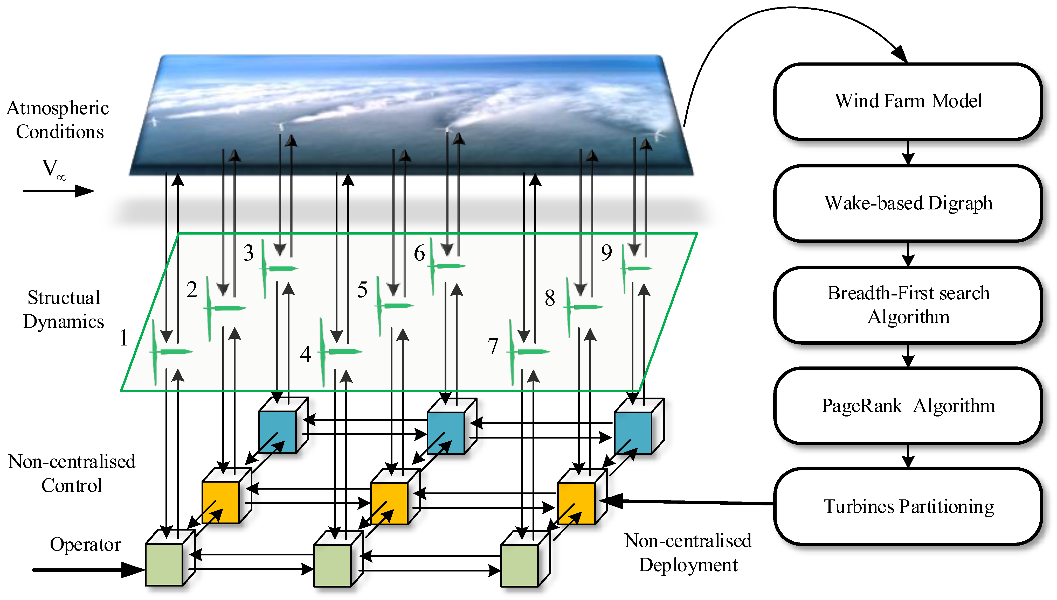
A non-centralised control strategy is designed by partitioning the wind farm into a number of uncoupled subsets of turbines. In other words, wind turbines are grouped into subsets depending on their wake effect coupling levels. We explore an edge propagation sparse graph strategy to divide the wind farm into several uncoupled partitions using the BFS and PageRank centrality computation algorithms. The turbine partitioning process mainly consists of a wind farm model, wake-based digraph generation, breadth-first search algorithm, PageRank algorithm, and turbine partitioning, as shown in Figure 3.

3.1. Finding Subgraph Using the BFS Algorithm

Inter-turbine wake propagation couplings can be represented like a digraph G = V , E , W , where nodes V represent the turbines, edges E represent the wake interaction strength between turbines, the adjacency matrix W represents whether node-edge pairs are incident or not, and its degree matrix, which contains information about the degree of each node [20]. Furthermore, let m = { 1,2 , , M } be the set of indices for m Z 0 partitions P m of the digraph G and {T1,…, TN} be the number of turbines within each subgraph G s = ( V s , E s , W s ) that is a tree covering clustering subsets of turbines with all edges.
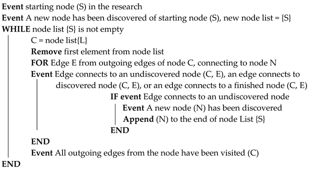
The m-partitioning problem requires starting to find the subgraph G s = ( V s , E s , W s ) using the BFS algorithm [36]. The BFS algorithm begins at the starting node, s, and inspects all of its neighbouring nodes in order of their node index. Then, it visits its unvisited neighbours for each of those neighbours in the wake-based graph G . The algorithm continues until all nodes and edges that are reachable from the starting node have been visited, which the algorithm finds a subgraph G s of starting node S. Notably, here, in the wake-based digraph G , we define the starting nodes (lead turbines) to have zero in-degree. Lead turbines are T1, T2, and T3, and specific analysis is provided in Section 5.1. In pseudo-code, the BFS algorithm can be implemented as Algorithm 1:
Algorithm 1: The BFS algorithm finds the subgraph of a lead turbine.
Energies 16 07131 i001

3.2. Calculating and Ranking the PageRank Score of Subgraphs

There may be shared nodes between different subgraphs, so the partition can not be completely decoupled. Therefore, we introduced a PageRank centrality computation algorithm to calculate the PageRank score of shared turbines and to determine which belongs to which subgraph.
The PageRank centrality computation algorithm was originally designed to rank search engine results in directed graphs or networks. For the weighted wake-based digraph, we applied this algorithm to calculate turbine j and PageRank score P R j to evaluate the relative importance of turbine j ’s neighbours, i , to the centrality of turbine j by the degree of j . The formula is expressed as [37]:
P R j = μ i   A i j v i d i + β
This definition can be written in matrix form as:
P R = β I μ D 1 A 1
where D is a diagonal matrix and D j j is the degree of turbine j (in a weighted digraph, W is used instead, where the diagonal w j j is the strength of turbine j), μ denotes the damping factor μ r a n d [ 0 , 1 ] , β denotes the preassigned constant centrality value, A represents the adjacency matrix of weighted wake-based digraph G . In this case, the parameters μ and β are 0.85 and 1, respectively.
The PageRank centrality computation algorithm calculated and ranked the PageRank score of the shared turbines in the corresponding subgraphs. The PageRank score indicates the degree of importance of the shared turbine in a subgraph. Theoretically, the higher score of the shared turbine demonstrates that it is more connected and its centrality within the corresponding subgraph, which the shared turbine will retain in the subgraph with the highest PR score.

3.3. Partitioning Using the Edge Propagation Graph Sparse Strategy

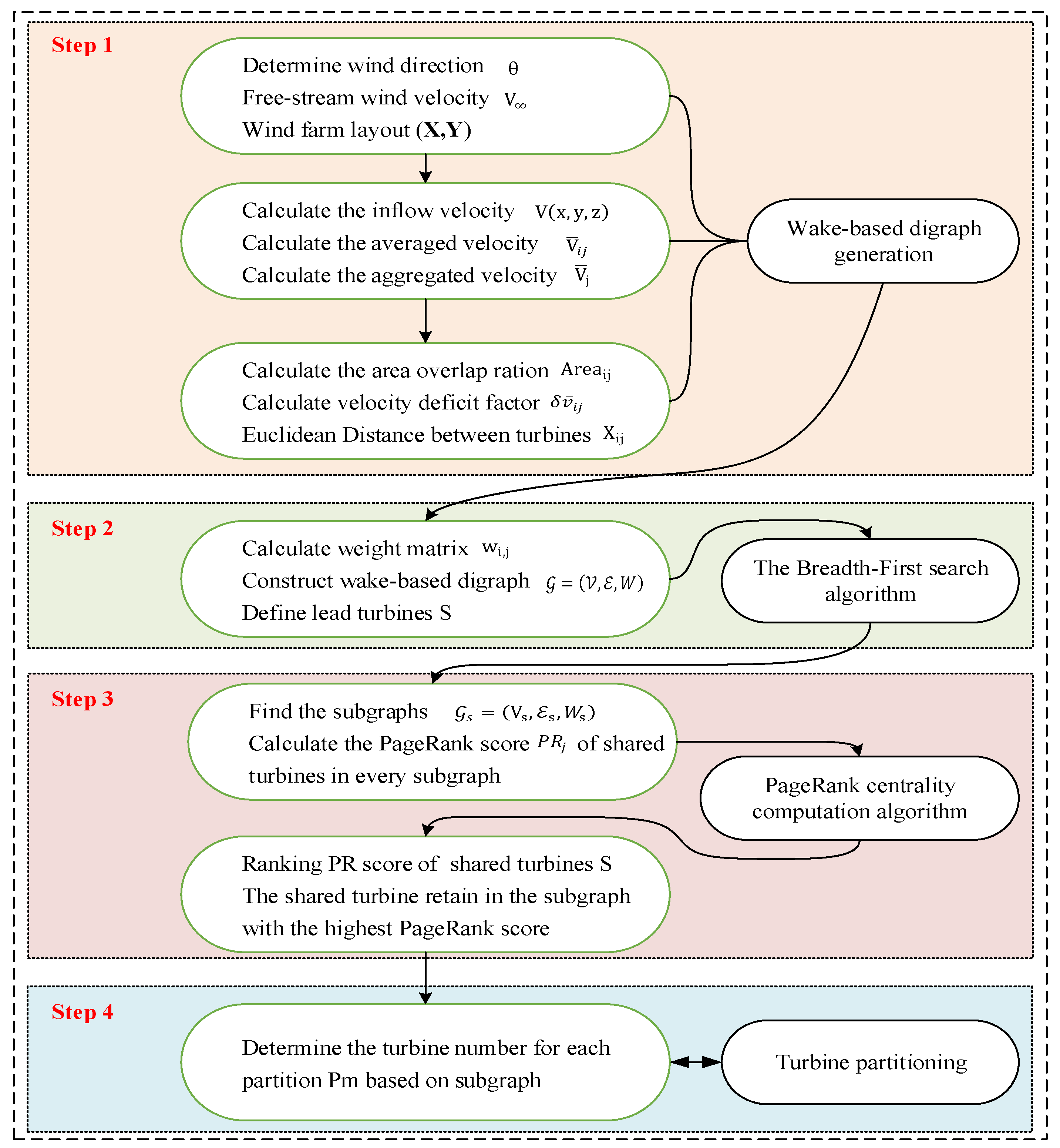
For a set of wind directions θ = θ 1 , , θ w , there are m-partitioning P m for each angle θ θ . Assuming a given direction θ has a corresponding partitioning P m = P 1 , , P M , where M is the number of partitioning, and m = { 1 , , M } . As a result of this, based on the wind farm layout ( X , Y ) , we construct the original wake digraph G and calculate the weight coefficient matrix W to determine the communication neighbourhood of turbines. Once m sub-digraphs G s = V s , E s , A s is searched, and the P R j score of the shared turbines is calculated. Specifically, Figure 4 illustrates different components involved in implementing and evaluating turbine partitioning through the edge propagation sparse graph strategy. The simulation studies we have carried out in this work consist of four major activities: wake-based digraph generation, finding the subgraph via the BFS algorithm, calculating and ranking P R j scores to determine the shared turbines belong to which subgraphs using the PR algorithm, and turbine partitioning.
Nevertheless, different atmospheric conditions lead to different turbine partitioning results. On the other hand, turbulence and atmospheric conditions are sensitive to the wind direction in order to select the appropriate turbine subset of partitions based on the effective wind direction.

3.4. A Nine-Turbine Case for Turbine Partitioning

As discussed in the above section, we demonstrate the procedure for turbine partitioning using the proposed strategy. We consider the WF layout with three-by-three turbines, as depicted in Figure 5a, in the values of θ = 30 , V = 8   m / s , and T I = 0.05 . The wake original digraph G and adjacency matrix W are illustrated in Figure 5b,c.
To define the lead turbine, the degree of a turbine (node) provides information on wake interaction between upstream turbines and downstream turbines. For example, turbine T1 with zero in-degree indicates it is unaffected by the wake of the upstream turbines. That is, it experiences freestream velocity V , then T1 is defined as the lead node of a subgraph. In this case, there are three lead nodes (T1, T2, and T3, respectively), which means that three subgraphs can be found in digraph G , as illustrated in Figure 5b.
Table 1 illustrates the process for finding the subgraph of a lead turbine T2 using the BFS algorithm. Reading the events in Table 1 from top to bottom will help you understand the algorithm. As a result of the search, the node numbers indicate the order in which they appeared, which is 2 → 5 → 8 → 9, and the discovered edge is the found subgraph of lead turbine T2. As shown in Figure 5d, we found three subgraphs, G s 1 ,   G s 2 ,   a n d   G s 3 , corresponding to T1, T2, and T3. Notably, there are shared nodes, T8, that belong to both G s 1 and G s 2 , and T9 belongs to both G s 2 and G s 3 . Those subgraphs can not be completely decoupled, and further decomposition is needed.
Figure 5e shows the process of calculating and ranking the P R j scores of three subgraphs using the centrality computation algorithm, which determines that the shared turbine T8 belongs to the subgraph G s 2 , and T9 belongs to the subgraph G s 3 . For the shared turbine T8, in the subgraph G s 1 and G s 2 , its PR score is 0.19051 and 0.38482, respectively. The higher score demonstrates that turbine T8 is more important and central for the subgraph G s 2 compare to subgraph G s 1 . As a result, T8 is retained in the subgraph G s 2 . Similar analyses have been made for turbine T9.
The results are illustrated in Figure 5f, illustrating the partitioning subgraph topology. The final turbine partitioning produces the following: the lead turbine is T1, T2, and T3, respectively. The decoupled turbine partitioned subsets are P1 = {T1|T4, T7}, P2 = {T2|T5, T8}, and P3 = {T3|T6, T9}.

4. Problem Formulation and Optimisation

The fatigue loading of wind turbines will lead to fatigue damage to its structure, reduce its life, increase the risk of failure, affect their performance and efficiency, and increase the cost of their maintenance and operation. For wind turbines, reasonable design and control of fatigue load is one of the important measures to ensure the safe and reliable operation of wind turbines [38,39,40]; therefore, the load-balancing power dispatch strategy has been designed. In the area of wind farm control, the MPPT and maximising the total output power of the wind farm control strategy are widely used. Under the MPPT strategy, there is no restriction on the production of energy by each turbine since it operates independently. However, the wake effect on downstream turbines and uneven fatigue distribution of the wind farm will be exacerbated.
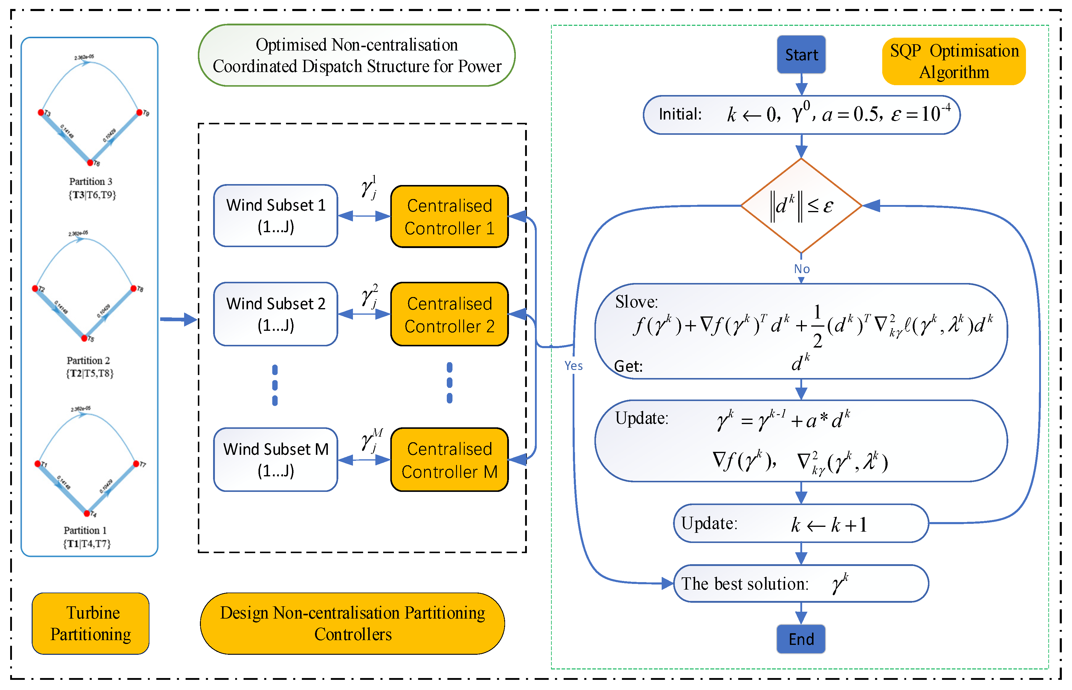
The strategy that maximises the total output power of wind farms can increase power production by mitigating the wake effect. It still does not consider the uneven fatigue distribution of turbines to cause high maintenance frequency and a high cost. In view of this, the non-centralised optimised power dispatch strategy is proposed to maximise the power production while minimising the fatigue loading distribution on the wind farm. In short, the coordinated dispatch process has three stages: turbine partitioning, design of non-centralisation partitioning controllers, and SQP optimisation algorithm, as shown in Figure 6.

4.1. Optimisation Problem

For a given decoupled m-partitioning P m and m = { 1 , , M } , which have j number of turbines and j = { 1 , , J } . By doing so, multiple individual non-centralisation partitioning controllers control the overall WF, in which the sequential quadratic programming (SQP) optimisation algorithm is applied to achieve optimised yaw angles γ k , and k is the number of iterations. The fatigue load-balancing power control objectives function of non-centralisation partitioning controllers are defined as follows:
  • maximising the whole production of electricity from wind farms:
    max γ P W F = m = 1 M j = 1 J   P j m γ j ; V ¯ j   ;
  • minimising the wind farm standard deviation of the fatigue loading:
    min γ F s t d = 1 M J m = 1 M j = 1 J   F j m γ j ; V ¯ j F ¯ j m γ j ; V ¯ j 2 .
Hence, except for output power, the optimised power dispatch (OPD) strategy proposes a penalty function that is included as part of the loss function to reflect the distribution of fatigue loads:
min γ f ( γ ) = P W F + α F s t d
s t : b ( γ ) = γ j γ m i n 0 γ m a x γ j 0 P rate   P j 0 F rate   F j 0
where α is the penalty factor in accordance with the magnitude of F s t d (the detail of α choice is discussed in Section 5.4) with the value set at 100, γ m i n and γ m a x represent the minimum and maximum yaw angles range, P rate denotes rated power, and F rate denotes the rated mechanical fatigue loads. Notably, when the penalty factor α is set to 0, Equation (11) degenerates to maximise the power control strategy.

4.2. Optimisation Method

The OWF non-centralised optimisation function is a nonlinear programming (NLP) problem, which employs an SQP algorithm is used to determine the optimal yaw angles settings. Each partitioning P m concludes a small number of turbines in the OWF are independent of one another and may solve their optimisation problems simultaneously. This inequality-constrained optimisation problem (11) is converted into a Lagrangian equation:
L ( γ , λ ) = f ( γ ) λ b ( γ ) ,
where λ are Lagrange multipliers. At an iterate γ k , a basic sequential quadratic programming algorithm defines an appropriate search direction d k as a solution to the quadratic programming subproblem:
min d k f ( γ k ) + f ( γ k ) T d k + 1 2 ( d k ) T k γ 2 L ( γ k , λ k ) d k
s . t .     b ( γ k ) + d k ( γ k ) T d k 0
Note that the term f ( γ k ) in the expression above may be left out for the minimisation problem since it is constantly under the minimise d k operator. This sequential quadratic programming (SQP)algorithm uses gradient f ( γ k ) and the inverse Hessian k γ 2 L ( γ k , λ k ) is used to guide the search through the design space, and this method does not necessarily ensure that a global optimum will be found. In spite of this, results will indicate that optimised yaw angles γ k settings result in better performance, the detailed optimisation process is shown in Figure 6.

5. Validations and Discussion

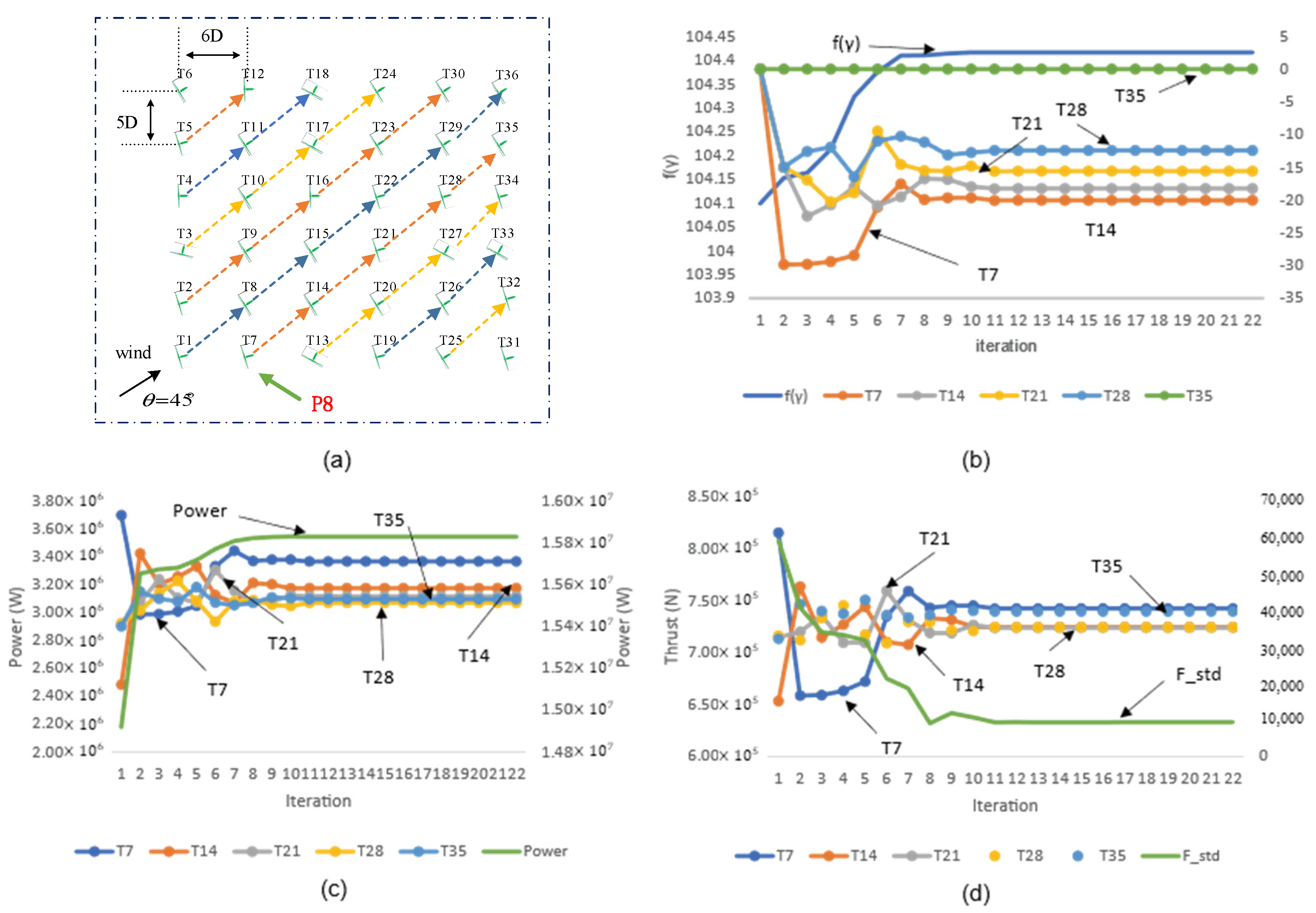
This section uses a rectangular WF with 36 DTU-10 MW turbines to verify the newly proposed strategy. Despite the wind farm’s layout, all turbines are 5D apart along their x-axis, whereas 6D apart along their y-axis, as shown in Figure 7a. Under different wind directions, winds speeds, and turbulence intensities, wind field and wake effects are simulated using the FLOw Redirection and Induction in Steady State (FLORIS), which is an open-source wind plant optimisation tool complemented by the FLORIS-based Analysis for Supervisory Control and data acquisition tool. In this paper, the yaw angles are set as γ i n i t i a l = 0 and γ 30 , 30 . After the wind turbines are partitioned into several uncoupled subsets, a series of simulations are conducted based on these subsets to verify three strategies:
  • Strategy A: MPPT strategy of WF power [41];
  • Strategy B: centralised fatigue load-balancing power dispatch strategy [42] (the wind turbines in the wind farm are not partitioned);
  • Strategy C: non-centralised fatigue load-balancing power dispatch strategy (the wind turbines in the wind farm are partitioned).
Accordingly, simulation studies have been conducted for the following cases: (1) turbine partitioning, (2) control of a wind farm with only one wind direction in mind, (3) power efficiency and fatigue distribution of wind farms is expected to improve, and (4) discussion of the penalty factor α . Notably, all optimisation strategies were implemented on a desktop computer and executed serially.

5.1. Turbine Partitioning

Considering the atmospheric condition as wind direction θ = 45 , an effective freestream speed V = 9   m / s , and turbulence intensity T I = 0.05 , the same calculation process described in the above section shows the partitioning results shown in Figure 7, Table 2 and Table 3, and Figure 8.
Figure 7 demonstrates the decomposition process of the wake-based graph, including the layout of the WF with 36 turbines, wake-based digraph, and 11-subgraphs. The wake-based digraph is shown in Figure 7b and found 11-subgraphs are shown (S1, S2, S3, S4, S5, S6, S7, S8, S9, S10, and S11).
Five subgraphs (S5, S6, S7, S8, and S9) can not be completely decoupled, and Table 2 explains the shared turbines attribution process and results. The data from Table 2 represent the P R j scores of the shared turbines (T24, T30, T23, T35, T29, and T36) in subgraphs (S5, S6, S7, S8, and S9), respectively. The bold turbines of each row correspond to the highest score of the shared turbine and are retained in the corresponding subgraph. For example, shared turbine T36 belonged to both S8 and S9, and the higher score demonstrates that turbine T36 is more important and central for the subgraph S9 than for S8. Therefore, T36 is retained in S3, corresponding decoupled partitioned subsets P9. As a result, the 11-partitioned subsets are as follows: the lead turbine is T 31 , T 19 , T 6 , T 4 , T 3 , T 2 , T 13 , T 7 , T 1 , T 25 , and T 5 , respectively. A further point to be made is that the number of turbines in the partitioning subset did not exceed 8.

5.2. Wind Farm Control Considering a Single Wind Direction

For partitioned subsets, this figure shows the results of the yaw optimisation process using the non-centralised SQP algorithm (strategy C). Accordingly, eleven non-centralised SQP algorithms parallel operations are carried out, aiming to both maximise output power and minimising fatigue distribution standard deviation by the wind turbines in the given partitioned subsets. The maximisation in each partitioned subset total production of electricity can be obtained, as well as the fatigue distribution standard deviation in terms of the whole wind farm. As shown in Figure 8a, the partitioned subset P 8 : { T 7 | T 14 , T 21 , T 28 , T 35 } is considered. Figure 8b–d shows how the control actions and loss function f ( γ ) , P ( γ ) , F _ s t d ( γ ) of the wind turbine will converge to the optimum values by non-centralised SQP iterations. As part of the SQP process, wind turbines adjust the yaw angle to maximise the loss function f ( γ ) and P ( γ ) of the partitioned subset P 8 in spite of a decrease in their own power production, as for the lead turbine T7, the F _ s t d ( γ ) continuously decreases. In the subsequent iterations, the power of all cluster subsets in the overall wind farms keeps increasing due to coordinated optimisation control actions, until it reaches its optimum value.
In general, for optimal yaw angle distributions, the power distribution within the wind farms tends to be more homogeneous as the first turbine’s power is decreased and the downstream turbine’s power is increased.
Table 3 shows the captured power and fatigue distribution simulation results of three strategies. It is evident from the results that the WF captured power and fatigue thrust loads of strategy A are the smallest, and the fatigue distribution is the maximum. Due to the yaw of wind turbines, the power produced is minimal. Only the first exhaust wind turbines are capable of producing significant power (see Figure 9a,b). The power and fatigue thrust generated by units in the upstream direction are at their maximum, while the power and fatigue thrust generated by units in the downstream direction are significantly reduced. The output power and fatigue thrust of the WF utilising strategy B is maximal and the results of fatigue distribution are the best. As compared to strategy A, strategy B’s output power decrement is less than 0.7362 MW; the fatigue thrust increase from B to C is less than 0.2258 MN. The fatigue distribution of Strategy C is 1.21 times larger than that of strategy B, and 33.91% of strategy A. However, the computational time of strategy C shows a great improvement, which is 60.99% of strategy B. Considering together the computational time, output power, and fatigue distribution perspective, strategy C is better than strategies B and A. Notably, the output power and fatigue thrust are inversely proportional to fatigue variance. In other words, the output power and fatigue thrust loads can be controlled by fatigue distribution variance.
To obtain more information from Figure 9, the output power and fatigue thrust loads reference distributions using three strategies are compared. Compared to strategy A, both strategy B and C increase the output power and decrease fatigue distribution reference of downstream WTs by derating upstream WTs. Strategy B is the global optimisation of all WTs in the whole wind farm; the variance of fatigue distribution is smaller and the output power and fatigue distribution are more uniform, as shown in Figure 9c,d. The optimisation of strategy C is based on each partition, which is global optimisation for the partitioned turbines and sub-optimisation for the wind farms. Because of this, the variance of fatigue distribution of strategy C increases, while the output power and fatigue thrust decrease compared with strategy B, as shown in Figure 9e,f. However, strategy C derates the computer time less, even though the maximum captured power cannot be obtained this way. It is not difficult to find that the power increment of strategy C is sacrificed in order to achieve a high computational speed. As a result of strategy C, WF can yield the maximum energy while incorporating fatigue distribution into the calculation.

5.3. Expected Improvement in the Wind Farm

For different wind directions Φ = { 0 o , 5 o , 10 o , 15 o , , 175 o , 180 o } , generally, wind regions are classified as follows: low-velocity V 8   m / s , medium-speed V 11.4 m / s , high-speed V 18 m / s , and high-velocity, which compares the gain evolution of output power, standard fatigue deviation, and thrust loads resulting from strategies A, B, and C. The gain variation curves (B−A)/A and (C−A)/A are drawn to make a clear comparison. We demonstrate the results of the simulation in Figure 10, Table 4 and Table 5.
Figure 10a–c are the gain variation curves of output power for different wind directions. According to the picture, strategy B consistently produces the greatest power gain, and power curve of strategy C that is quite similar to strategy B. Furthermore, there is a relationship between wind direction and the power gain improvement. If wind directions are θ = 0 o , 45 o , 90 o , 145 o , a n d   180 o , there is an increase in power production of over 9% compared to other wind directions. This is because the distance in those directions between two WTs is shorter, leading to a stronger wake effect. In other words, the yaw angle of turbines creates more optimisation space to improve power gain. The curves of standard deviations of variations in fatigue are associated with the wind velocity, as described three strategies above, and are, respectively, shown in Figure 10d–f. It is clear that strategies B and C can achieve a smaller fatigue standard deviation than strategy A for the three wind velocities. While V = 8   m / s and V = 11.4   m / s , the decrease in standard fatigue deviation increases the gain of power. Once V = 18   m / s , the wake velocity V i as described in Equation (1) of each WT reaches to V r a t e d , in other words, V i V r a t e d . Although the standard deviation decreases, the power gain value is zero (Figure 10c), which is unwilling to be seen. Therefore, the proposed optimisation method is not suitable for high-velocity regions.
Figure 10g–i are the gain variation curves of fatigue loads in different directions. Figure 10 shows that algorithms B and C produced fatigue loads greater than strategy A, indicating that the thrust loading increases with the increase of power production. Furthermore, the gain curves characteristic of thrust load vary consistently with the change law of gain variation curves of output power. When Φ = 45 o , 135 o , 225 o , a n d   315 o , the gains of thrust loads are more than in other wind directions.
Table 4 shows the total power gain and the standard deviation of fatigue and thrust loads in three wind velocity regions. It is seen that the WF captured the power of strategy A is the smallest and achieves the largest standard fatigue deviations. The power gain obtained is inversely proportional to the wind velocity, and the thrust loads increase with the increase in power production. Specifically, under the low-velocity V = 8   m / s region, the total power gain is 3.75%, 3.25%, and thrust loads is 0.36%, 0.02% using strategies B and C, respectively. In the near-rated velocity 11.4 m / s region, the gains of output power are 2.11% and 1.77%, and the gains of thrust loads are 0.96% and 0.95%. While under high-velocity region 18 m / s , the gains of output power are always 0%, and the output power become a constant value (rated output power). It means that under the higher velocity region, the lower the wake-based yaw angle optimisation effect, even if the standard fatigue deviation decreases. Notably, under the high-velocity region of 18 m/s, the total thrust loads generated are smaller than that near-rated velocity region of 11.4 m/s. The reason is that in the high-velocity region, the power coefficient and thrust coefficient will become smaller to keep the turbines working at the rated power (see Figure 2b,c).
On the other hand, the standard deviation of fatigue loading is extremely important. Most WTs will require less maintenance if their standard deviations are balanced, and it is possible to repair them all with one maintenance. Thus, maintenance frequency can be reduced and maintenance costs can be saved by maintaining a balanced standard deviation of fatigue. In addition, strategies B and C demonstrate that balancing fatigue distribution and increasing captured energy do not always conflict with one another. Therefore, at little energy cost, one can maintain a low fatigue deviation.
Table 5 results show that strategy C may be suitable for real-time computing, although strategy B always captures the maximum wind energy. Strategy C’s captured power gain is less than the Strategy B approach. Still, it shortens the calculation time significantly, consuming only about 50% of the total time taken by Strategy B in the three velocity regions. Moreover, Strategy C results in a power gain loss of only 0.5%, 0.33%, and 0% compared to Strategy B. Calculation accuracy is decreased by Strategy C in order to improve calculation speed. Further, compared with Strategy B, the results of Strategy C have no significant power computational loss, indicating that the turbine partitioning retains the most critical wake relationship of the wind farm.

5.4. Discussion of the Penalty Factor

Following the case study, the output power sensitivity analysis was performed, and the standard deviation of when the wind velocity is 9 m/s with a 35° wind direction, fatigue against the penalty factor α is carried out on a WF with 9 turbines (see Figure 5a). By using the OPD loss function, we can calculate the WF’s output power increments and the standard deviation of fatigue reductions (Equation (11)), and the results under these wind conditions are shown in Figure 11. Using the picture as an example, it is obvious that by increasing α , the standard deviation reduces while the power decreases. Hence, it is possible to increase the power increment by choosing a small α and the standard deviation with more beneficial fatigue by choosing a large α ; however, a compromised result might be desired by the operator. In this scenario, the value of α that is above the MPPT and OPD power curves’ intersect region is a good choice (the choice located with the red rectangle α [0, 160]), because in this range, the power has been improved, and the standard deviation of fatigue is relatively small. It turns out that the relationship between the power increment curve and fatigue distribution curve is pretty complicated, and it will be affected by the wind speed and direction as well. To decide how to set the value of α , it is recommended that the value be determined by comparing the simulated increment curve for output power and the fatigue loading normal deviation curve under the current wind condition.

6. Conclusions

As a result of this paper, a novel approach has been presented for power dispatch in wind farms that aims to control the fatigue loading on wind turbines, so that the accumulated fatigue loading over the operational lifetime is balanced as much as possible. As for guaranteeing real-time control for large wind farms, an edge propagation sparse graph turbine partitioning strategy has been used where each turbine is divided into decoupling subsets that are individually controlled by local controllers. Later on, conventional approaches were introduced and compared with the non-centralised load-balancing power dispatch strategy. As a result of the simulation, the proposed strategy appears to be effective and can reduce computational costs and improve wind farm power production, in which accumulated fatigue loading over the operational lifetime was balanced as much as possible. The present study allows for conclusions as following to be drawn:
  • Using the edge propagation sparse graph method, a large wind farm can divide into multiple smaller turbine partitioning subsets. The breadth-first search and PageRank centrality computation algorithm were appropriately applied to reduce computation complexity while preserving the important wake coupling relationship between turbines;
  • The non-centralised and centralised load-balancing control strategy can increase power production and reduce fatigue standard deviations more than the MPPT strategy does under low-velocity and rated-velocity regions. Nevertheless, there will be a small increase in fatigue of turbines due to the increase in power production;
  • However, it is required to balance the accumulated fatigue loading over the wind farm so that the different wind turbines experience similar levels of fatigue loading to reduce maintenance frequency. According to the results, the proposed non-centralised coordination optimisation using SQP algorithm is capable of solving the combined non-convex OWF problems;
  • Compared to centralised fatigue load-balancing, the non-centralised strategy consistently reduces calculation time. The whole wind farm optimisation problem is split into several sub-problems, which provide a method to solve the “dimension cruise” of large-scale wind farms.
In the Future, investigation work should focus on deploying the algorithm in the distributed system, which can speed up the algorithm optimisation process. In addition, it would be worthwhile to explore a more intelligent partitioning approach considering wake effects in future research.

Author Contributions

Conceptualization, T.S. and Y.H.J.; methodology, T.S.; software, T.S.; validation, T.S.; formal analysis, T.S.; investigation, T.S.; resources, T.S.; data curation, T.S.; writing—original draft preparation, T.S.; writing—review and editing, Y.H.J.; visualization, Y.H.J.; supervision, Y.H.J.; project administration, Y.H.J.; funding acquisition, Y.H.J. All authors have read and agreed to the published version of the manuscript.

Funding

This work was supported in part by the Basic Science Research Program under Grant NRF-2016R1A6A1A03013567 and Grant NRF-2021R1A2B5B01001484 and by the framework of International Cooperation Program under Grant NRF-2022K2A9A2A06045121 through the National Research Foundation of Korea (NRF) funded by the Ministry of Education.

Data Availability Statement

Data available in a publicly accessible repository that does not issue DOIs. Publicly available datasets were analyzed in this study. This data can be found here: [https://github.com/NREL/floris].

Conflicts of Interest

The authors declare no conflict of interest.

References

  1. Hosseinzadeh, S.; Etemad-Shahidi, A.; Stewart, R.A. Site Selection of Combined Offshore Wind and Wave Energy Farms: A Systematic Review. Energies 2023, 16, 2074. [Google Scholar] [CrossRef]
  2. Martínez-Gordón, R.; Sánchez-Diéguez, M.; Fattahi, A.; Morales-España, G.; Sijm, J.; Faaij, A. Modelling a highly decarbonised North Sea energy system in 2050: A multinational approach. Adv. Appl. Energy 2022, 5, 100080. [Google Scholar] [CrossRef]
  3. Enevoldsen, P.; Jacobson, M.Z. Data investigation of installed and output power densities of onshore and offshore wind turbines worldwide. Energy Sustain. Dev. 2021, 60, 40–51. [Google Scholar] [CrossRef]
  4. Boersma, S.; Doekemeijer, B.M.; Gebraad, P.M.O.; Fleming, P.A.; Annoni, J.; Scholbrock, A.K.; Frederik, J.A.; van Wingerden, J.-W. A tutorial on control-oriented modeling and control of wind farms. In Proceedings of the IEEE 2017 American Control Conference (ACC), Seattle, WA, USA, 24–26 May 2017; pp. 1–18. [Google Scholar]
  5. Kheirabadi, A.C.; Nagamune, R. A quantitative review of wind farm control with the objective of wind farm power maximization. J. Wind Eng. Ind. Aerodyn. 2019, 192, 45–73. [Google Scholar] [CrossRef]
  6. Hur, S. Modelling and control of a wind turbine and farm. Energy 2018, 156, 360–370. [Google Scholar] [CrossRef]
  7. Annoni, J.; Bay, C.; Taylor, T.; Pao, L.; Fleming, P.; Johnson, K. Efficient Optimization of Large Wind Farms for Real-Time Control. In Proceedings of the IEEE 2018 Annual American Control Conference (ACC), Milwaukee, WI, USA, 27–29 June 2018; pp. 6200–6205. [Google Scholar]
  8. Hagen, L.V.; Petrick, K.; Wilhelm, S.; Schmehl, R. Life-Cycle Assessment of a Multi-Megawatt Airborne Wind Energy System. Energies 2023, 16, 1750. [Google Scholar] [CrossRef]
  9. Siniscalchi-Minna, S.; Bianchi, F.D.; Ocampo-Martinez, C.; Domínguez-García, J.L.; De Schutter, B. A non-centralized predictive control strategy for wind farm active power control: A wake-based partitioning approach. Renew. Energy 2020, 150, 656–669. [Google Scholar] [CrossRef]
  10. Asim, T.; Islam, S.; Hemmati, A.; Khalid, M. A Review of Recent Advancements in Offshore Wind Turbine Technology. Energies 2022, 15, 579. [Google Scholar] [CrossRef]
  11. Dongran, S.; Liu, J.; Yang, Y.; Yang, J.; Su, M.; Wang, Y.; Gui, N.; Xuebing, Y.; Huang, L.; Joo, Y.H. Maximum wind energy extraction of large-scale wind turbines using nonlinear model predictive control via Yin-Yang grey wolf optimization algorithm. Energy 2021, 221, 119866. [Google Scholar] [CrossRef]
  12. Liao, H.; Hu, W.; Wu, X.; Wang, N.; Liu, Z.; Huang, Q.; Chen, C.; Chen, Z. Active power dispatch optimization for offshore wind farms considering fatigue distribution. Renew. Energy 2020, 151, 1173–1185. [Google Scholar] [CrossRef]
  13. Song, D.; Tu, Y.; Wang, L.; Jin, F.; Li, Z.; Huang, C.; Xia, E.; Rizk-Allah, R.M.; Yang, J.; Su, M.; et al. Coordinated optimization on energy capture and torque fluctuation of wind turbines via variable weight NMPC with fuzzy regulator. Appl. Energy 2022, 312, 118821. [Google Scholar] [CrossRef]
  14. Gebraad, P.M.O.; van Wingerden, J.W. Maximum power-point tracking control for wind farms: Maximum power-point tracking control for wind farms. Wind Energy 2015, 18, 429–447. [Google Scholar] [CrossRef]
  15. Gionfra, N.; Sandou, G.; Siguerdidjane, H.; Faille, D.; Loevenbruck, P. Wind farm distributed PSO-based control for constrained power generation maximization. Renew. Energy 2019, 133, 103–117. [Google Scholar] [CrossRef]
  16. Zhong, S.; Wang, X. Decentralized Model-Free Wind Farm Control via Discrete Adaptive Filtering Methods. IEEE Trans. Smart Grid 2018, 9, 2529–2540. [Google Scholar] [CrossRef]
  17. Huang, S.; Wu, Q.; Guo, Y.; Lin, Z. Bi-level decentralized active and reactive power control for large-scale wind farm cluster. Int. J. Electr. Power Energy Syst. 2019, 111, 201–215. [Google Scholar] [CrossRef]
  18. Chen, Y.; Joo, Y.H.; Song, D. Multi-Objective Optimisation for Large-Scale Offshore Wind Farm Based on Decoupled Groups Operation. Energies 2022, 15, 2336. [Google Scholar] [CrossRef]
  19. Chen, Y.; Joo, Y.-H.; Song, D. Modified Beetle Annealing Search (BAS) Optimization Strategy for Maxing Wind Farm Power through an Adaptive Wake Digraph Clustering Approach. Energies 2021, 14, 7326. [Google Scholar] [CrossRef]
  20. Shu, T.; Song, D.; Hoon Joo, Y. Decentralised optimisation for large offshore wind farms using a sparsified wake directed graph. Appl. Energy 2022, 306, 117986. [Google Scholar] [CrossRef]
  21. Shu, T.; Song, D.; Joo, Y.H. Non-centralised coordinated optimisation for maximising offshore wind farm power via a sparse communication architecture. Appl. Energy 2022, 324, 119705. [Google Scholar] [CrossRef]
  22. Li, Q.; Su, Y.; Tan, M. Coordinative optimization on fatigue distribution and active power in wind farms. IEEE 2016 International Symposium on Electrical Engineering (ISEE), Hong Kong, China, 4 December 2016; pp. 1–6. [Google Scholar]
  23. Zhang, B.; Soltani, M.; Hu, W.; Hou, P.; Huang, Q.; Chen, Z. Optimized Power Dispatch in Wind Farms for Power Maximizing Considering Fatigue Loads. IEEE Trans. Sustain. Energy 2018, 9, 862–871. [Google Scholar] [CrossRef]
  24. Zhao, H.; Wu, Q.; Huang, S.; Shahidehpour, M.; Guo, Q.; Sun, H. Fatigue Load Sensitivity-Based Optimal Active Power Dispatch For Wind Farms. IEEE Trans. Sustain. Energy 2017, 8, 1247–1259. [Google Scholar] [CrossRef]
  25. Data-Driven Control (TU Delft). 2021. Available online: https://github.com/TUDelft-DataDrivenControl/FLORISSE_M (accessed on 18 April 2021).
  26. Qian, G.-W.; Ishihara, T. Wind farm power maximization through wake steering with a new multiple wake model for prediction of turbulence intensity. Energy 2021, 220, 119680. [Google Scholar] [CrossRef]
  27. Gao, X.; Li, B.; Wang, T.; Sun, H.; Yang, H.; Li, Y.; Wang, Y.; Zhao, F. Investigation and validation of 3D wake model for horizontal-axis wind turbines based on filed measurements. Appl. Energy 2020, 260, 114272. [Google Scholar] [CrossRef]
  28. Doekemeijer, B.M.; van der Hoek, D.; van Wingerden, J.-W. Closed-loop model-based wind farm control using FLORIS under time-varying inflow conditions. Renew. Energy 2020, 156, 719–730. [Google Scholar] [CrossRef]
  29. Park, J.; Park, J. Physics-induced graph neural network: An application to wind-farm power estimation. Energy 2019, 187, 115883. [Google Scholar] [CrossRef]
  30. Wen, J.; Zhou, L.; Zhang, H. Mode interpretation of blade number effects on wake dynamics of small-scale horizontal axis wind turbine. Energy 2023, 263, 125692. [Google Scholar] [CrossRef]
  31. Doekemeijer, B.; van Wingerden, J. Observability of the ambient conditions in model-based estimation for wind farm control: A focus on static models. Wind Energy 2020, 23, 1777–1791. [Google Scholar] [CrossRef]
  32. Bastankhah, M.; Porté-Agel, F. Experimental and theoretical study of wind turbine wakes in yawed conditions. J. Fluid Mech. 2016, 806, 506–541. [Google Scholar] [CrossRef]
  33. Bastankhah, M.; Porté-Agel, F. A new analytical model for wind-turbine wakes. Renew. Energy 2014, 70, 116–123. [Google Scholar] [CrossRef]
  34. Park, J.; Law, K.H. Cooperative wind turbine control for maximizing wind farm power using sequential convex programming. Energy Convers. Manag. 2015, 101, 295–316. [Google Scholar] [CrossRef]
  35. Dou, B.; Qu, T.; Lei, L.; Zeng, P. Optimization of wind turbine yaw angles in a wind farm using a three-dimensional yawed wake model. Energy 2020, 209, 118415. [Google Scholar] [CrossRef]
  36. Zhang, Y.; Zang, W.; Zheng, J.; Cappietti, L.; Zhang, J.; Zheng, Y.; Fernandez-Rodriguez, E. The influence of waves propagating with the current on the wake of a tidal stream turbine. Appl. Energy 2021, 290, 116729. [Google Scholar] [CrossRef]
  37. Muggiasca, S.; Taruffi, F.; Fontanella, A.; Di Carlo, S.; Giberti, H.; Facchinetti, A.; Belloli, M. Design of an aeroelastic physical model of the DTU 10MW wind turbine for a floating offshore multipurpose platform prototype. Ocean Eng. 2021, 239, 109837. [Google Scholar] [CrossRef]
  38. Skiena, S.S. Sorting and Searching. In The Algorithm Design Manual; Springer: London, UK, 2012; pp. 103–144. ISBN 978-1-84800-069-8. [Google Scholar]
  39. Oldham, S.; Fulcher, B.; Parkes, L.; Arnatkevičiūtė, A.; Suo, C.; Fornito, A. Consistency and differences between centrality measures across distinct classes of networks. PLoS ONE 2019, 14, e0220061. [Google Scholar] [CrossRef] [PubMed]
  40. Gu, B.; Meng, H.; Ge, M.; Zhang, H.; Liu, X. Cooperative multiagent optimization method for wind farm power de-livery maximization. Energy 2021, 233, 121076. [Google Scholar] [CrossRef]
  41. Gebraad, P.M.O.; Teeuwisse, F.W.; Van Wingerden, J.W.; Fleming, P.A.; Ruben, S.D.; Marden, J.R.; Pao, L.Y. Wind plant power optimization through yaw control using a parametric model for wake effects a CFD simulation study: Wind plant optimization by yaw control using a parametric wake model. Wind Energ. 2016, 19, 95–114. [Google Scholar] [CrossRef]
  42. Van Dijk, M.T.; Van Wingerden, J.-W.; Ashuri, T.; Li, Y. Wind farm multi-objective wake redirection for optimizing power production and loads. Energy 2017, 121, 561–569. [Google Scholar] [CrossRef]
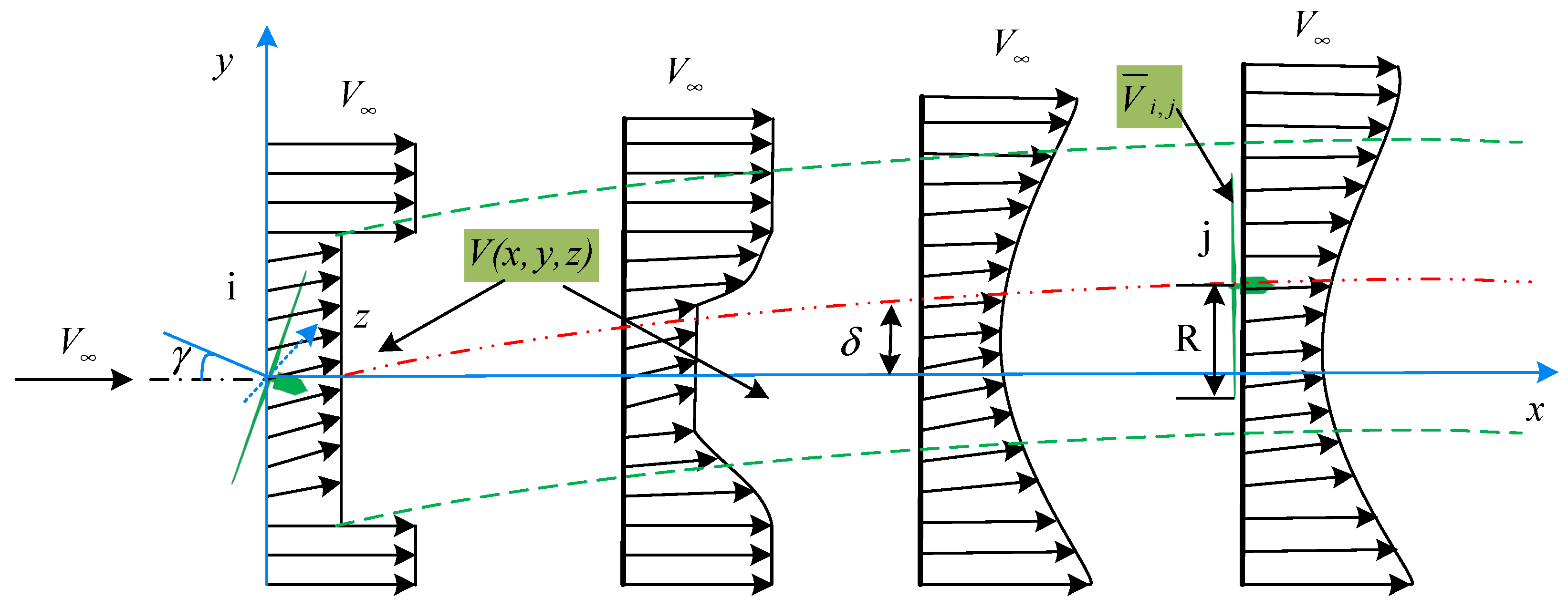
Figure 1. Calculating the steady-state wind velocity V x , y , z and the averaged velocity V ¯ i , j , where γ denotes the yaw angle of the upstream turbine, δ denotes the wake deflection, the green lines denote the wake of the upstream turbine under yawed conditions, and the red line indicates the wake centreline.
Energies 16 07131 g001
Figure 2. Aggregated velocity and coefficient curves. (a) Calculating the aggregated velocity V ¯ j ; (b) power coefficient curves to the wind speeds and yaw angles; (c) thrust coefficient curves to the wind speeds and yaw angles.
Energies 16 07131 g002
Figure 3. The process of turbine partitioning for non-centralised control deployment (Numbers 1–9 represent wind turbines, these colorful boxes represent different wind turbines controller).
Energies 16 07131 g003
Figure 4. Calculation flow chart of partitioning using the edge propagation sparse graph strategy.
Energies 16 07131 g004
Figure 5. Nine-turbine example of partitioning processes using the edge propagation sparse graph strategy. (a) Wake field. (b) Wake-based digraph G (Turbines T1, T2, and T3 are marked with a green circle to indicate lead turbines whose in-degree is zero; turbines T8 and T9 indicate shared turbines marked with solid green circles). (c) Adjacency matrix W (dark green marking for shared turbines T8 and T9, numerical values represent the wake strength). (d) Finding three subgraphs ( G s 1 ,   G s 2 ,   a n d   G s 3 ) . (e) Calculating and ranking PR scores. (f) Three partitions of turbines ( P 1 ,   P 2   a n d   P 3 ).
Energies 16 07131 g005
Figure 6. The optimised non-centralised coordinated dispatch structure for power.
Energies 16 07131 g006
Figure 7. Subgraphs of the WF with 36 turbines ( θ = 45 , V = 9   m / s , T I = 0.05 ). (a) The layout of the WF with 36 turbines. (b) A wake-based digraph and 11-subgraphs (S1, S2, S3, S4, S5, S6, S7, S8, S9, S10, and S11) (the green mark indicates the shared turbine T23, T24, T29, T30, T35, and T36).
Energies 16 07131 g007
Figure 8. Progression of the f ( γ ) , P ( γ ) , F _ s t d ( γ ) for five selected WTs of partitioned P8 with the iterations of proposed algorithm ( Φ = 45 o ). (a) A schematic diagram of turbine partitioning. (b) Trajectories of the yaw angels and loss function f ( γ ) . (c) Trajectories of the individual and total output power P ( γ ) . (d) Trajectories of the individual fatigue thrust loads and F _ s t d ( γ ) .
Energies 16 07131 g008
Figure 9. The output power and fatigue thrust loads using three strategies (the red dotted emphasizes the first row and column of wind turbines). (a) Strategy A’s output power. (b) Strategy A’s output fatigue thrust loads. (c) Strategy B’s output power. (d) Strategy B’s output fatigue thrust loads. (e) Strategy C’s output power. (f) Strategy C’s output fatigue thrust loads.
Energies 16 07131 g009
Figure 10. The gain variation curves of output power, standard fatigue deviation, and thrust loads resulting from strategies B and C with different wind directions (The spacing of the rings varies uniformly and represents a fixed gain). (a) Output power in V = 8   m / s ; (b) output power in V = 11.4   m / s ; (c) output power in V = 18   m / s ; (d) standard fatigue deviation in V = 8   m / s ; (e) standard fatigue deviation in V = 11.4   m / s . (f) standard fatigue deviation in V = 18   m / s ; (g) thrust loads in V = 8   m / s ; (h) thrust loads in V = 11.4   m / s ; (i) thrust loads in V = 18   m / s . Results are expressed in % change to strategy A.
Energies 16 07131 g010
Figure 11. The sensitivity analysis output power and standard deviation of the fatigue against the value of penalty factor α.
Energies 16 07131 g011
Table 1. The process for finding the subgraph of a lead turbine T2.
StepEventNodeEdge
Start NodeEnd Node
1Starting node 2.2
2Discover a new node 2.2
3Discover an edge between node 2 and node 5. 25
4Discover a new node 5.5
5Discover an edge between node 2 and node 8. 28
6Discover a new node 8.8
7Discover an edge between node 2 and node 9. 29
8Discover a new node 9.9
9Starting from node 2, it visits all outgoing edges.2
10Previously discovered nodes (5 and 8) are connected by an edge. 58
11Previously discovered nodes (5 and 9) are connected by an edge. 59
12Starting from node 5, it visits all outgoing edges.5
13Starting from node 8, it visits all outgoing edges.8
14Starting from node 9, it visits all outgoing edges.9
Table 2. Turbine partitioned results and PR scores of shared turbines (bold is the highest score).
Subgraph SubsetsPR ScoresPartitioned Subsets
S 1 : { T 31 | } P 1 : { T 31 | }
S2:{T19|T26,T33} P2:{T19|T26,T33}
S 3 : { T 6 | } P 3 : { T 6 | }
S4:{T4|T11,T18} P4:{T4|T11,T18}
S5:{T3|T10,T17,T24}T24:0.3742P5:{T3|T10,T17,T24}
S6:{T2|T9,T16,T23,T24,T30}T23:0.2354
T24:0.0763
T30:0.2834
P6:{T2|T30,T23,T16,T9}
S7:{T13|T20,T27,T34,T35}T35: 0.1053P7:{T13|T20,T27,T34}
S8:{T7|T14, T21,T28,T29,T35,T36}T29:0.0670
T35:0.2479
T36: 0.1251
P8:{T7|T14,T21,T28,T35}
S9:{T1|T8,T15,T22,T23,T29,T30,T36}T23:0.0528
T29:0.1890
T30:0.0985
T36:0.2195
P9:{T1|T8,T15,T22,T29,T36}
S10:{T25|T32} P10:{T25|T32}
S11:{T5|T12} P11:{T5|T12}
Table 3. Simulation results of three strategies.
StrategyOutput Power (MW)Fatigue Distribution ( F s t d )Fatigue Thrust (MN)Computational Time (S)
A109.53726.2596 ×   10 4 26.27780.1663
B115.51040.9579 ×   10 4 26.6392436.3909
C114.77422.1228 ×   10 4 26.4134266.1419
Table 4. The increased rate of the total wind farm output power, standard fatigue deviation, and fatigue loads obtained under strategies A, B, and C (the sum of all angles). The increased rate is expressed in % and calculated as the baseline of the values from strategy A.
Wind Speed (m/s)Strategy AStrategy BStrategy C(B−A)/A(C−A)/A
Output Power (W)84.1209 ×   10 9 4.2659 ×   10 9 4.2467 ×   10 9 3.75%3.25%
11.41.1537 ×   10 10 1.1760 ×   10 10 1.1724 ×   10 10 2.10%1.77%
181.3320 ×   10 10 1.3320 ×   10 10 1.3320 ×   10 10 0.00%0.00%
Fatigue Std82.2814 ×   10 6 7.0534 ×   10 5 9.9224 ×   10 5 −61.29%−49.96%
11.42.6728 ×   10 6 1.2532 ×   10 6 1.3845 ×   10 6 −34.77%−32.45%
184.4428 ×   10 5 1.4848 ×   10 5 3.1529 ×   10 4 −94.57%−63.12%
Thrust loads (N)89.8307 ×   10 8 9.8639 ×   10 8 9.8312 ×   10 9 0.36%0.02%
11.41.8324 ×   10 9 1.8494 ×   10 9 1.8491 ×   10 9 0.96%0.95%
181.0630 ×   10 9 1.0691 ×   10 9 1.1454 ×   10 9 0.57%7.72%
Table 5. Calculation time of the strategies A, B, and C. (average of all angles).
Wind SpeedCalculation Time (s)
Strategy AStrategy BStrategy C
8 m/s0.1652391.4392209.4987
11.4 m/s0.1503215.9121127.6709
18 m/s0.1616395.4584201.5212
Disclaimer/Publisher’s Note: The statements, opinions and data contained in all publications are solely those of the individual author(s) and contributor(s) and not of MDPI and/or the editor(s). MDPI and/or the editor(s) disclaim responsibility for any injury to people or property resulting from any ideas, methods, instructions or products referred to in the content.